Classical and quantum nonlinear optical information processing

(1)

Classical and Quantum Nonlinear Optical Information Processing

Thesis by

Mankei Tsang

In Partial Fulfillment of the Requirements for the Degree of

Doctor of Philosophy

California Institute of Technology Pasadena, California

2006

(2)

c

2006

(3)

Acknowledgements

First and foremost I would like to thank my mentor, Professor Demetri Psaltis, for giving me the opportunity to come to Caltech and for his insightful advice about optics, research, and all aspects of life in academia. It has truly been a pleasure working with him in my four years at Caltech.

I would also like to acknowledge my past and present group mates, who are all intelligent and capable, and from whom I have learned a great deal. I am especially grateful to Dr. Ye Pu and Dr. Martin Centurion, for their guidance when I worked briefly in the lab and for sharing with me their exciting experiment results; Jim Adleman and Dr. David Erickson, for all the driving in a long but enjoyable road trip to the DARPA workship in Sonoma; Lucinda Acosta, for her help in administrative tasks; and Yayun Liu, for her words of encouragement when I first started at Caltech. Furthermore, I would like to acknowledge Dr. Zhiwen Liu, Dr. Hung-Te Hsieh, Zhenyu Li, Hua Long, Troy Rockwood, Eric Ostby, Xin Heng, Baiyang Li, Dr. Allen Pu, Jae-Woo Choi, and Ted Dikaliotis, with whom I have enjoyed countless inspiring discussions.

I am indebted to Dr. Fiorenzo Omenetto, who provided his experimental results for my first paper, and generously lent us his experimental equipment several times; Professor Michael Cross, for his advice on the metaphoric optical computing project; and my candidacy and thesis examining committee members, includ-ing Professor Amnon Yariv, Professor Changhuei Yang, Professor Oskar Painter, Professor Kerry Vahala, and Dr. John Hong, for their valuable time, as well as their insightful feedback on my research.

I will forever be indebted to my mother, whose love, care, and support make me the person I am now, despite all the adversities she has had to face. I am also grateful to my elder sister, and all my relatives and friends in Hong Kong and the United States, who are extremely supportive of my family and myself.

(4)

List of Publications

[1] M. Tsang and D. Psaltis, “Dispersion and nonlinearity compensation by spectral phase conjugation,” Opt. Lett. 28, 1558 (2003).

[2] M. Tsang, D. Psaltis, and F. G. Omenetto, “Reverse propagation of femtosecond pulses in optical fibers,” Opt. Lett. 28, 1873 (2003).

[3] M. Tsang and D. Psaltis, “Spectral phase conjugation with cross-phase modulation compensation,” Opt. Express 12, 2207 (2004).

[4] M. Tsang and D. Psaltis, “Spectral phase conjugation by quasi-phase-matched three-wave mixing,” Opt. Commun. 242, 659 (2004).

[5] M. Tsang and D. Psaltis, “Spontaneous spectral phase conjugation for coincident frequency entangle-ment,” Phys. Rev. A 71, 043806 (2005).

[6] M. Centurion, Y. Pu, M. Tsang, and D. Psaltis, “Dynamics of filament formation in a Kerr medium,” Phys. Rev. A 71, 063811 (2005).

[7] M. Tsang, “Spectral phase conjugation via extended phase matching,” J. Opt. Soc. Am. B 23, 861 (2006).

[8] M. Tsang and D. Psaltis, “Propagation of temporal entanglement,” Phys. Rev. A 73, 013822 (2006).

[9] M. Tsang, “Quantum temporal correlations and entanglement via adiabatic control of vector solitons,” e-print quant-ph/0603088 [submitted to Phys. Rev. Lett. ].

[10] M. Tsang and D. Psaltis, “Reflectionless evanescent wave amplification via two dielectric planar wave-guides,” e-print physics/0603079 [submitted to Opt. Lett. ].

[11] M. Tsang, “Beating the spatial standard quantum limits via adiabatic soliton expansion and negative refraction,” under preparation.

(5)

Abstract

This thesis is a theoretical investigation of the classical and quantum information processing enabled by the advent of modern ultrafast nonlinear optics.

Chapter 2 and 3 study the propagation of ultrashort optical pulses in optical fibers, and propose two meth-ods of compensating the linear and nonlinear distortions experienced by the pulses, namely, reverse propaga-tion and spectral phase conjugapropaga-tion. Chapter 4 and 5 suggest different schemes that implement spectral phase conjugation.

Chapter 6 and 7 establish the connection between classical spectral phase conjugation and quantum co-incident frequency entanglement. Chapter 6 shows how a spectral phase conjugator can create coco-incident frequency entangled photon pairs, and Chapter 7 in turn demonstrates how a coincident frequency entangle-ment generator can perform spectral phase conjugation.

The next three chapters, 8, 9, and 10, focus on quantum spatiotemporal information processing. Chapter 8 studies the temporal properties of entangled photon pair propagation and proposes the concept of quantum temporal imaging. Chapter 9 investigates how optical solitons can be used to perform quantum timing jitter reduction and temporal entanglement, while Chapter 10 applies the same idea to the spatial domain for quantum spatial information processing tasks, such as spatial beam displacement uncertainty reduction and quantum lithography.

(6)

List of Figures

2.1 Comparison of OPC and reverse propagation. . . 5 2.2 Reverse propagation of an experimental output pulse. The experimental output pulse shape is

plotted at z=0 m and numerically propagates in reverse from z=0 m to z=−10 m. . . 6 2.3 Comparison of the input obtained from reverse propagation and the actual experimental input. 7 2.4 Reverse propagation of a chirped sech pulse atλ0=1550 nm. . . 8 2.5 Amplitude and phase of the optimal input that produces the desired sech output pulse shape at

λ0=800 nm. . . 9 2.6 Compared with the ideal output pulse shape produced by reverse propagation and pulse

shap-ing, the OPC output is significantly distorted by high-order effects. . . 9

3.1 Schematics of TPC and SPC. . . 12 3.2 Input and output pulses with and without compensation schemes, when a 1.7 W 200 fs

super-Gaussian pulse propagates for a total distance of 2 km. . . 16 3.3 Input and output pulses with and without compensation schemes, when multiple 17 W 200 fs

solitons propagates for a total distance of 1 km. . . 17

4.1 Setup of SPC by four-wave mixing. As(t)is the signal pulse, Ap(t)and Aq(t)are the pump pulses, and Ai(t)is the backward-propagating idler pulse. (After Ref. [1]) . . . 20 4.2 (a) Amplitude and (b) phase of output idler (solid lines) Ai(−L₂,t)compared with input signal

(dash lines) As(−L₂,t). XPM is neglected in this example. As predicted, the output idler is time-reversed and phase-conjugated with respect to the input signal. Parameters used are

n2=1×10−11cm2/W, n0=1.7,λ0=800 nm, L=2 mm, d=5µm, Ts= 1 ps, Tp= 100 fs,

Ep= 12.8 nJ, pump fluence =E_Ldp. Conversion efficiency is 100%. . . 27 4.3 Conversion efficiencies from simulations compared with predictions from first-order

(11)

4.4 (a) and (b) plot the normalized amplitude and phase of the output idler Ai(−L₂,t)compared to the SPC of the input signal A∗_s(−L

2,−t), respectively, when XPM is present. The amplitude plots are normalized with respect to their peaks. The output idler is distorted and the conversion efficiency is only 34%, much lower than the theoretical efficiency 100%. (c) and (d) plot the same data, but with XPM compensation. The efficiency is back to 100% and the accuracy is restored. . . 29 4.5 Plots of amplitude and phase of one pump pulse with ideal phase adjustment according to

Eq. (4.57) in the time and frequency domain. Top-left: temporal envelope; bottom-left: tempo-ral phase; top-right: envelope spectrum; bottom-right: specttempo-ral phase. The simple pulse shape should be easily produced by many pulse shaping methods. . . 29 4.6 Amplitude and phase of output idler and input signal for the wave mixing process, with a signal

energy of 5 nJ, much above the pump depletion limit, to demonstrate the effect of pump depletion. 31

5.1 Geometry of SPC by quasi-phase-matched three-wave mixing. As(t)is the incoming signal pulse with a carrier frequencyω0, and Ap(t)is the second-harmonic pump pulse. Ai(t)is the generated idler pulse. Quasi-phase matching is achieved by aχ(2)grating with periodΛalong x. 34 5.2 Plots of intensity and phase of incoming signal and output idler from numerical analysis. It is

clear from the plots that the idler is a phase-conjugated and time-reversed replica of the signal, confirming our theoretical derivations. Parameters used areχ(2)=50 pm/V, n0=3, L=1 mm,

d=5µm, width in y=d, Ep=2.1µJ, pump fluence=E_Ldp. For such dimensions waveguide confinement of the signal and the idler is necessary. . . 38 5.3 Theoretical conversion efficiency derived from Eq. (5.17) and that from numerical analysis

plotted against pump energy. See caption of Fig. 5.2 for parameters used. . . 39

6.1 Spontaneous SPC by TWM. . . 43 6.2 Spontaneous SPC by FWM. . . 43

7.1 Schematic of spectral phase conjugation (SPC) via type-II extended phase matching (EPM). The signal and idler pulses, in orthogonal polarizations, have carrier frequencies ofωsandωi, while the pump pulse has a carrier frequency ofωp=ωs+ωi. The EPM condition requires that the signal and the idler counterpropagate with respect to the pump, which should be much shorter than the input signal. . . 54 7.2 Normalized poles p_∞/(χAp0) plotted against G, obtained by numerically solving Eq. (32),

indicating the onset of spatial instability beyond the threshold G>π/2. More poles appear as

(12)

7.3 Plots of intensity and phase of input signal, output signal, and output idler, from numerical analysis of Eqs. (5) and (6). Parameters used are k′_p=1/(1.5_×108_ms−1₎_{, k}′

s=1.025k′p,

ki=0.975k′p, Tp=100 fs, Ts=2 ps, L=10 cm, ts=4Ts, beam diameter = 200µm, As0= 0.5 exp[−(t₋2Ts)2/(2Ts2)]−exp[−(1+0.5 j)(t+2Ts)2/(2Ts2)], Ap0=exp[−t2/(2Tp2)], and

G=π/4. The plots clearly show that the idler is the time-reversed and phase-conjugated replica, i.e., SPC, of the signal. . . 62 7.4 Signal gainη+1 and idler gainη versus G from numerical analysis compared with theory.

See caption of Fig. 3 for parameters used. . . 62 7.5 Plot of numerical idler gainη in dB against G for L=10 cm (solid) and L=1 cm

(dash-dot), compared with the Fourier theory (dash), tan2(G)in dB. Three distinct regimes can be observed for the L=10 cm case; the moderate gain regime where the Fourier theory is accurate, the unstable regime where the gain increases exponentially, and the oscillation regime where significant pump depletion occurs. For L=1 cm, the medium is not long enough for oscillation to occur in the parameter range of interest. . . 63

8.1 Two-dimensional sketches of the two-photon probability amplitude before and after one of the photons is time-reversed. Uncertainty in arrival time difference is transformed to uncertainty in mean arrival time. . . 73 8.2 A quantum temporal imaging system for quantum-enhanced clock synchronization. . . 74 8.3 The quantum destructive interference via a coupler is determined by the overlap (dark grey

area) of the two-photon amplitudeψ12(0,t,0,t′)with its mirror image with respect to the t+t′ axis,ψ12(0,t′,0,t). . . 76 8.4 Quantum dispersive spreading of mean arrival time of a two-photon vector soliton. The

cross-phase modulation effect only preserves the two-photon coherence time, giving rise to temporal entanglement with positive time correlation. One can also manipulate the coherence time in-dependently by adiabatically changing the nonlinear coefficient along the propagation axis. . . 81

9.1 Proposed setup of generating multiphoton states with quantum-enhanced mean position ac-curacy via adiabatic control of vector solitons. A pulse is coupled into a vector soliton in a multimode nonlinear waveguide, in which dispersion adiabatically increases or the Kerr non-linearity adiabatically decreases. A second waveguide with an opposite dispersion is used for compensating the quantum dispersive spreading of the mean position. . . 88

(13)

11.1 Reflectionless evanescent wave amplification (REWA) by two slab waveguides, where n1>n0. 106 12.1 Intensity (left column), phase (middle column), and phase gradient (right column) of two

opti-cal vortex solitons with the same charge (top row), which should rotate in the same sense, and those of two vortex solitons with opposite charges, which should drift in a direction perpendic-ular to their separation. The phase gradient near the centers of the vortices is not plotted due to its divergence. . . 118 12.2 Sketches of velocity and flux of a vortex blob and an optical vortex along a line across the

center, to illustrate the similarities between the two in terms of the flux. . . 120 12.3 Comparison between a viscous boundary layer and an optical boundary layer. . . 123 12.4 Setup of numerical experiment (not to scale). . . 124 12.5 The intensity of the optical beam at a normalized propagation distanceζ =10, forM ₌0.4

andR₌12.8. The dark ellipse is the low-refractive-index region that acts as an impenetrable object. Optical vortex solitons are seen to be created on the top and bottom side of the ellipse, While the convection of the solitons behind the object resembles the twin vortices behind an obstacle in a viscous fluid flow. . . 124 12.6 A vector plot of the flux J atζ=10, forM ₌₀_._{4 and}R₌₁₂_._{8, which confirms the similarity}

between the numerically observed dynamics and the phenomenon of twin vortices. . . 125 12.7 A plot of the momentum vorticity∇_×J atζ =10, forM ₌₀_._{4 and}R₌₁₂_._{8. A white dot}

indicates that the vortex has a positive topological charge and a black dot indicates that the vortex has a negative charge. The plot shows the similarity between the numerically observed dynamics and the phenomenon of twin vortices. . . 125 12.8 The intensity of the optical beam at a normalized propagation distanceζ =20, forM ₌0.4

andR₌12.8. The qualitative dynamical behavior is essentially unchanged from that shown in Fig. 12.5. . . 126 12.9 A vector plot of the flux J atζ =20, forM ₌₀_._{4 and}R₌₁₂_._{8. . . 126} 12.10 A plot of the momentum vorticity∇_×J atζ=20, forM₌₀_._{4 and}R₌₁₂_._{8. . . 126} 12.11 The optical intensity atζ=10, forM ₌₀_._{4 and}R₌₂₅_._{6. The vortex solitons are observed}

to be smaller, and the phenomenon of twin vortices is again observed. . . 127 12.12 The flux J atζ=10, forM₌₀_._{4 and}R₌₂₅_._6. _{. . . 127} 12.13 The momentum vorticity∇_×J atζ=10, forM ₌0.4 andR₌25.6. . . 127 12.14 Optical intensity atζ =20, forM ₌0.4 andR₌25.6. The twin vortices become unstable

and detach alternatively from the object. . . 128 12.15 Flux atζ=20, forM ₌0.4 andR₌25.6, which shows a flow pattern strongly resembling

(14)

(15)

List of Tables

(16)

Chapter 1

Summary

This thesis investigates various classical and quantum optics techniques for applications in optical communi-cations, quantum information processing, imaging, and computing.

Chapter 2 presents a numerical technique for reversing femtosecond pulse propagation in an optical fiber, such that given any output pulse it is possible to obtain the input pulse shape by numerically undoing all dispersion and nonlinear effects. The technique is tested against experimental results, and it is shown that it can be used for fiber output pulse optimization in both the anomalous and normal dispersion regimes [1].

Chapter 3 proposes the use of spectral phase conjugation to compensate for dispersion of all orders, self-phase modulation, and self-steepening of an optical pulse in a fiber. Although this method cannot compensate for loss and intrapulse Raman scattering, it is superior to the previously suggested midway temporal phase conjugation method if high-order dispersion is a main source of distortion. The reshaping performance of our proposed scheme and a combined temporal and spectral phase conjugation scheme in the presence of uncompensated effects is studied numerically [2].

Chapter 4 analyzes spectral phase conjugation with short pump pulses in a third-order nonlinear material in depth. It is shown that if signal amplification is considered, the conversion efficiency can be significantly higher than previously considered, while the spectral phase conjugation operation remains accurate. A novel method of compensating for cross-phase modulation, the main parasitic effect, is also proposed. The validity of our theory and the performance of the spectral phase conjugation scheme are studied numerically [3].

Chapter 5 proposes a novel spectral phase conjugation scheme by three-wave mixing. It is shown that a phase-conjugated and time-reversed replica of the incoming signal can be generated, if appropriate quasi-phase matching is achieved and the three-wave mixing process is transversely pumped by a short second-harmonic pulse [4].

(17)

Chapter 7 demonstrates that the copropagating three-wave-mixing parametric process, with appropriate type-II extended phase matching and pumped with a short second-harmonic pulse, can perform spectral phase conjugation and parametric amplification, which shows a threshold behavior analogous to backward wave oscillation. The process is also analyzed in the Heisenberg picture, which predicts a spontaneous parametric down conversion rate in agreement with experimental results reported elsewhere [6].

Chapter 8 derives the equations that govern the temporal evolution of two photons in the Schr¨odinger picture, taking into account the effects of loss, group-velocity dispersion, temporal phase modulation, linear coupling among different optical modes, and four-wave mixing. Inspired by the formalism, the concept of quantum temporal imaging is proposed, which uses dispersive elements and temporal phase modulators to manipulate the temporal correlation of two entangled photons. The exact solution of a two-photon vector soliton is also presented, in order to demonstrate the ease of use and intuitiveness of the proposed formulation [7].

Chapter 9 shows that optical pulses with a mean position accuracy beyond the standard quantum limit can be produced by adiabatically expanding an optical vector soliton followed by classical dispersion man-agement. The proposed scheme is also capable of entangling positions of optical pulses and can potentially be used for general continuous-variable quantum information processing [8].

Chapter 10 studies spatial quantum enhancement effects under a unified framework. An approach of generating arbitrary quantum lithographic patterns by the use of multiphoton coincident momentum states is proposed. It is shown that the multiphoton absorption rate of photons with a quantum-enhanced lithographic resolution is reduced, not enhanced, contrary to popular belief. Finally, the use of adiabatic soliton expansion followed by negative refraction is proposed to beat both the standard quantum limit on the optical beam displacement accuracy, as well as that on the minimum spot size of quantum lithography [9].

(18)

Bibliography

[1] M. Tsang, D. Psaltis, and F. G. Omenetto, Opt. Lett. 28, 1873 (2003).

[2] M. Tsang and D. Psaltis, Opt. Lett. 28, 1558 (2003).

[3] M. Tsang and D. Psaltis, Opt. Express 12, 2207 (2004).

[4] M. Tsang and D. Psaltis, Opt. Commun. 242, 659 (2004).

[5] M. Tsang and D. Psaltis, Phys. Rev. A 71, 043806 (2005).

[6] M. Tsang, J. Opt. Soc. Am. B 23, 861 (2006).

[7] M. Tsang and D. Psaltis, Phys. Rev. A 73, 013822 (2006).

[8] M. Tsang, e-print quant-ph/0603088 [submitted to Phys. Rev. Lett. ].

[9] M. Tsang, under preparation.

[10] M. Tsang and D. Psaltis, e-print physics/0603079 [submitted to Opt. Lett. ].

(19)

Chapter 2

Reverse propagation of femtosecond

pulses in optical fibers

2.1

Introduction

Dispersion and nonlinear effects have been the bottleneck of ultrafast pulse propagation in an optical fiber. Various schemes, for example, optical solitons [1] and optical phase conjugation (OPC) [2, 3] have been pro-posed to compensate for these effects, yet the high-order distortions including third-order dispersion (TOD), self-steepening, and Raman scattering remain undefeated. Femtosecond power delivery in a normally dis-persive fiber, which is useful for biomedical applications, is especially difficult to achieve because normal dispersion and nonlinear effects always tend to broaden and distort a pulse. Another scheme is to embrace all the effects and adopt an adaptive optimization method, typically in the form of genetic algorithm, hoping that modulating the input pulse shape can produce an output with desirable properties [4, 5, 6]. Although an adaptive method can compensate for pulse propagation distortions and unknown experimental variables, it does not make full use of our theoretical knowledge of optical fiber ultrafast pulse propagation and may therefore be time consuming and suboptimal.

(20)

2.2

Theory

The nonlinear pulse propagation equation in a fiber is given by the general form [1]

∂A(z,T)

∂z ={Dˆ+Nˆ[A(z,T)]}A(z,T), (2.1)

where A(z,T)is the pulse envelope, ˆD is the linear operator that includes absorption and all dispersion effects,

and ˆN is the nonlinear operator that includes all nonlinear effects and is a function of A(z,T). Mathematically, the output is obtained by application of the propagation operator to the input:

A(L,T) =exp

n

L ˆD+ Z L

0 ˆ

N[A(z,T)]dz

o

A(0,T), (2.2)

where L is the length of the fiber. The input can also be expressed in terms of the output by application of the reverse propagation operator:

A(0,T) =expn₋L ˆD₋

Z L

0 ˆ

N[A(z,T)]dzoA(L,T). (2.3)

To solve this equation and derive the input pulse shape given the output, we use the standard Fourier split-step method:

A(z,T)≈exp(−h ˆD)exp_{−h ˆN[A(z+h,T)]}A(z+h,T), (2.4)

in each step of which the linear and nonlinear effects on a pulse shape are evaluated separately for a small propagation distance h.

Figure 2.1: Comparison of OPC and reverse propagation.

As a comparison, let us consider the OPC technique in the operator notation. Figure 2.1 depicts schemat-ically the OPC method and the reverse propagation method. By conjugating Eq. (2.2) and comparing the result with Eq. (2.3), one can see that OPC can reconstruct an input pulse if ˆD and ˆN contain operators

(21)

self-steepening, that may severely hamper the accuracy of pulse reconstruction by OPC, especially in the femtosecond regime. In a numerical simulation of reverse propagation, however, there is no such limitation, and all effects can be included to yield the optimal input pulse shape.

To model femtosecond pulse propagation, we choose the linear operator ˆD to be

ˆ

D=−α 2 −j

β2 2

∂2

∂T2+

β3 6

∂3

∂T3. (2.5)

The first term corresponds to loss, the second term corresponds to group-velocity dispersion (GVD), and the third term corresponds to TOD. The higher-order dispersion terms are neglected because of the relatively short length considered here but can be easily included if the need arises.

The nonlinear operator ˆN is

ˆ

N=jγh_|A_|2+ j ω0

1

A

∂ ∂T(|A|

2_A₎ −TR∂|

A_|2

∂T

i

. (2.6)

The first term corresponds to optical Kerr effect, the second term corresponds to self-steepening, and the third term corresponds to intrapulse Raman scattering.

Figure 2.2: Reverse propagation of an experimental output pulse. The experimental output pulse shape is plotted at z=0 m and numerically propagates in reverse from z=0 m to z=−10 m.

2.3

Comparison with experiments

(22)

optical gating measurements we obtain the amplitude and phase of both input and output pulses. The output pulse is then reverse propagated in a computer simulation as in Fig. 2.2. The output pulse shape is plotted at

[image:22.612.171.478.184.432.2]

z=0 m at the top of the graph, and propagation effects are reversed numerically as the pulse goes from z=0 m to z=−10 m. The simulated input from reverse propagation is compared with the experimental input in Fig. 2.3. Both pulses are remarkably similar, with nearly identical amplitudes and positive chirp, showing that the reverse propagation theory is consistent with experimental results.

Figure 2.3: Comparison of the input obtained from reverse propagation and the actual experimental input.

2.4

Numerical analysis

(23)

[image:23.612.172.477.60.291.2]

Figure 2.4: Reverse propagation of a chirped sech pulse atλ0=1550 nm.

It must be stressed that the reverse propagation method is not limited to near-soliton conditions but can be applied to any fiber in both dispersion regimes. For our second numerical example consider a 1-m-long normally dispersive single-mode fiber atλ0=800 nm, with parametersβ2=40 ps2/km,β3=0.03 ps2/km, andγ=9 W−1km−1[8]. A 100-fs unchirped hyperbolic secant pulse, centered at 800 nm, with peak power

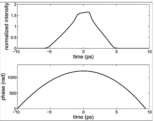
P0=20 kW and total energy E=4 nJ is given as our desired output. Figure 2.5 shows the optimal input pulse amplitude and phase. Qualitatively speaking, the pulse shape is asymmetric to compensate for TOD, self-steepening, and Raman scattering, and the negative chirp (C=−0.1 by polynomial fitting) focuses the pulse by GVD. In an experiment the large chirp can be imposed by a grating pair before 4 f pulse shaping.

We also investigate numerically the OPC technique, as depicted in Fig. (2.1), using the same criteria as those above as a comparison. Figure 2.6 shows the resultant output pulse by OPC compared with the ideal output pulse shape that can be produced by reverse propagation and pulse shaping. The OPC output pulse is distorted by high-order effects, whereas reverse propagation and pulse shaping, taking all the high-order effects into account, produce a better output.

2.5

Conclusion

(24)

Figure 2.5: Amplitude and phase of the optimal input that produces the desired sech output pulse shape at

[image:24.612.173.478.92.331.2]

λ0=800 nm.

(25)

(26)

Bibliography

[1] G. P. Agrawal, Nonlinear Fiber Optics (Academic, San Diego, Calif., 2001).

[2] A. Yariv, D. Fekete, and D. M. Pepper, Opt. Lett. 4, 52 (1979).

[3] R. A. Fisher, B. R. Suydam, and D. Yevick, Opt. Lett. 8, 611 (1983).

[4] R. S. Judson and H. Rabitz, Phys. Rev. Lett. 68, 1500 (1992).

[5] F. G. Omenetto, B. P. Luce, and A. J. Taylor, J. Opt. Soc. Am. B 16, 2005 (1999).

[6] F. G. Omenetto, A. J. Taylor, M. D. Moores, and D. H. Reitze, Opt. Lett. 26, 938 (2001).

[7] A. M. Weiner, J. P. Heritage, and E. M. Kirschner, J. Opt. Soc. Am. B 5, 1563 (1988).

(27)

Chapter 3

Dispersion and nonlinearity

compensation via spectral phase

conjugation

3.1

Introduction

Temporal phase conjugation (TPC) was proposed to compensate for group-velocity dispersion [1], self-phase modulation [2], and intrapulse Raman scattering [3] of an optical pulse in a fiber. However, when the pulse width is sufficiently short or the center wavelength is near the zero-dispersion point, third-order dispersion and self-steepening effects become more prominent and limit the reshaping performance of TPC. To compensate for the high-order effects, alternative methods [4, 5, 6, 7] have been suggested, but many of them are either too complicated or are only able to compensate for a limited number of propagation effects. An interesting scheme, which compensates for all effects by both TPC and a suitably chosen dispersion map, is also proposed by Pina et al. [8].

TPC

A(0,T) Fiber A(L,T) A*(L,T) Fiber A*(0,T)

SPC

A(0,T) Fiber A(L,T) A*(L,-T) Fiber A*(0,-T)

Figure 3.1: Schematics of TPC and SPC.

(28)

of the optical pulse in the frequency domain, hence the name spectral phase conjugation (SPC).

3.2

Theory

Consider a pulse E(t) =A(t)exp(−jω0t)with envelope A(t)and center frequencyω0. If we take the conju-gate of the Fourier transform of E(t), it becomes

˜

E∗(ω) = h Z ∞

−∞

A(t)exp(−jω0t)exp(jωt)dt

i∗

(3.1)

= Z ∞

−∞

A∗(−t)exp(−jω0t)exp(jωt)dt (3.2)

where the substitution t_{→ −}t is made. Hence, conjugation of individual spectral components of a pulse

is equivalent to phase conjugation and time reversal of the temporal envelope. TPC, on the other hand, corresponds to conjugation and inversion in the frequency domain.

Midway SPC is unique in the sense that it can compensate for all dispersion and most nonlinearities simultaneously. Consider the general pulse propagation equation in a fiber,

∂A(z,T)

∂z =

h

ˆ

DT+NˆT A(z,T)

i

A(z,T), (3.3)

where z is the propagation distance, T is the retarded time with respect to the group velocity 1/β1of the pulse (T =t₋β1z), and A(z,T)is the pulse envelope. ˆDT is the linear operator,

ˆ

DT =−α 2 +

∞

∑

n=2

jβn n!(j

∂ ∂T)

n_, _(3.4)

where the first term on the right-hand side is the loss term, and the remaining terms are nth-order dispersion terms. ˆNT is the nonlinear operator, which can be expressed as the following for a femtosecond pulse,

ˆ

NT(A) =jγ

h

|A_|2+ j ω0

1

A

∂ ∂T(|A|

2_A₎ −TR∂|

A_|2

∂T

i

, (3.5)

where the first term on the right-hand side is the phase modulation term, the second term is self-steepening, and the third term is intrapulse Raman scattering [9]. The subscript T of ˆDT and ˆNT denotes the derivatives with respect to T in the operators.

We rewrite Eq. (3.3) to express the output pulse in terms of the propagation operator applied to the input pulse [9],

A(L,T) =exphL ˆDT+ Z L

0 ˆ

NT A(z,T)dz

i

A(0,T), (3.6)

(29)

propagation operator [7],

A(0,T) =exph₋L ˆDT− Z L

0 ˆ

NT A(z,T)

dziA(L,T). (3.7)

Now let us take the complex conjugate of Eq. (3.7) and make the substitution T_{→ −}T . Eq. (3.7) becomes

A∗(0,−T) = exph₋L ˆD∗₋_T₋

Z L

0 ˆ

N₋∗_T A(z,−T)

dzi

A∗(L,−T). (3.8)

The conjugated and time reversed linear operator, ignoring loss, is

ˆ

D∗₋_T =

∞

∑

n=2 −jβn

n![(−j)(−

∂ ∂T)]

n _(3.9)

=

∞

∑

n=2 −jβn

n!(j

∂ ∂T)

n₌₋_D_ˆ

T. (3.10)

Similarly, the nonlinear operator, ignoring intrapulse Raman scattering, is

ˆ

N₋∗_T(A(z,−T)) = −_Nˆ_T₍_A∗₍_z_,₋_T₎₎_. _(3.11)

In general, we only keep terms that acquire a minus sign when conjugation and time reversal are both ap-plied. All operator terms, except loss and intrapulse Raman scattering, satisfy our criteria due to their odd combinations of j’s and time derivatives. With the substitution z_→L₋z′, Eq. (3.8) becomes

A∗(0,−T) = exphL ˆDT+ Z L

0 ˆ

NT A∗(L−z′,−T)dz′

i

A∗(L,−T). (3.12)

Eq. (3.12) has the exact same form as Eq. (3.6), but with A∗(L₋z′,−T)as the solution. In other words, if we launch A∗(L,−T)in another identical fiber, the final output A∗(0,−T)is a conjugated and time reversed version of the first input. This result can only be applied to cases where loss and intrapulse Raman scattering can be neglected. Table 3.1 summarizes the propagation effects that can be compensated by TPC and SPC, respectively.

loss EOD OOD SPM SS IRS

TPC _× √ _× √ _× √

SPC _× √ √ √ √ _×

(30)

To identify important propagation effects for a given optical pulse transmission system, it is useful to define a characteristic length for each propagation effect [9],

Lloss = loss length=1/α, (3.13)

LD = dispersion length=T02/|β2|, (3.14)

L′_D = third-order dispersion length=T₀3/|β3|, (3.15)

LNL = nonlinear length=1/(γP0), (3.16)

LSS = self-steepening length=ω0T0/(γP0), (3.17)

LR = Raman length=T0/(TRγP0), (3.18)

where T0is the pulse width. The significance of a propagation effect can be roughly estimated by the ratio of the total propagation distance Ltotalto the characteristic length. Hence a phase conjugation system should be designed such that the characteristic lengths of uncompensated propagation effects are much longer than

Ltotal. This is demonstrated next in the numerical simulations.

3.3

Numerical analysis

As a numerical example, considerλ0=1550 nm, two dispersion-shifted fibers, each with length Ltotal/2=1 km, parametersβ2=−1 ps2/km,β3=0.1 ps3/km,γ=1.5 W−1km−1,α=0.2 dB/km, TR=3 fs, a temporal or spectral phase conjugator in the middle, an amplifier at each fiber end to compensate for loss, and a super-Gaussian input pulse,

A(t) =p

P0exp[− 1 2(

T T0

)6_]_, _(3.19)

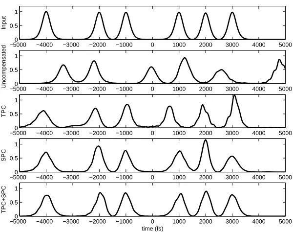
with T0=200 fs, and peak power P0=1.7 W. The peak power is chosen to be one-tenth of that of a funda-mental soliton, such that Lloss= 2 km, LD=0.04 km, LD′ =0.08 km, and LNL=0.4 km. Other characteristic lengths are too long to be significant. Since LNLis comparable to Ltotalwhile much longer than the dispersion lengths, we expect nonlinear effects to be observable but less significant than dispersion effects. The output pulses with and without compensation schemes are plotted in Fig. 3.2. SPC reconstructs the input pulse at the output almost perfectly, while the TPC output pulse is significantly distorted by third-order dispersion. At this power level, SPC has the advantage over TPC for the former’s ability to compensate for all important linear and nonlinear effects together with an amplifier.

(31)

broad-−5000 −400 −300 −200 −100 0 100 200 300 400 500 0.2

0.4 0.6 0.8 1

time (fs)

normalized intensity

input

uncompensated TPC

SPC

Figure 3.2: Input and output pulses with and without compensation schemes, when a 1.7 W 200 fs super-Gaussian pulse propagates for a total distance of 2 km.

ening is much slower than conventional pulses and the frequency of conjugation can be minimized. We note that periodic conjugation is also required in other schemes for different reasons, such as that suggested by Pina et. al., to satisfy the path-averaging assumption.

Since SPC can compensate for distortions not compensated by TPC, and vice versa, we propose that a hybrid scheme combining SPC and TPC can offer superior performance. An example would be to sandwich a temporal phase conjugator with two midway SPC systems, such that the Raman effect uncompensated in a SPC system can be compensated by the TPC system, at least to first order. More rigorous analysis is required to fully estimate the performance of a hybrid scheme.

(32)

−50000 −4000 −3000 −2000 −1000 0 1000 2000 3000 4000 5000 0.5

1

Input

−50000 −4000 −3000 −2000 −1000 0 1000 2000 3000 4000 5000 0.5

1

Uncompensated

−50000 −4000 −3000 −2000 −1000 0 1000 2000 3000 4000 5000 0.5

1

TPC

−50000 −4000 −3000 −2000 −1000 0 1000 2000 3000 4000 5000 0.5

1

SPC

−50000 −4000 −3000 −2000 −1000 0 1000 2000 3000 4000 5000 0.5

1

time (fs)

[image:32.612.174.474.69.306.2]

TPC+SPC

Figure 3.3: Input and output pulses with and without compensation schemes, when multiple 17 W 200 fs solitons propagates for a total distance of 1 km.

3.4

Conclusion

(33)

Bibliography

[1] A. Yariv, D. Fekete, and D. M. Pepper, Opt. Lett. 4, 52 (1979).

[2] R. A. Fisher, B. R. Suydam, and D. Yevick, Opt. Lett. 8, 611 (1983).

[3] S. Chi and S. F. Wen, Opt. Lett. 19, 1705 (1994).

[4] A. M. Weiner, D. E. Leaird, D. H. Reitze, and E. G. Paek, IEEE J. Quantum Electron. 28, 2251 (1992).

[5] C. Chang, H. P. Sardesai, and A. M. Weiner, Opt. Lett. 23, 283 (1998).

[6] F. G. Omenetto, A. J. Taylor, M. D. Moores, and D. H. Reitze, Opt. Lett. 26, 938 (2001).

[7] M. Tsang, D. Psaltis, and F. G. Omenetto, Opt. Lett. 28, 1873 (2003).

[8] J. Pina, B. Abueva, and G. Goedde, Opt. Commun. 176, 397 (2000).

[9] G. P. Agrawal, Nonlinear Fiber Optics (Academic Press, San Diego, 2001).

[10] D. A. B. Miller, Opt. Lett. 5, 300 (1980).

[11] D. Marom, D. Panasenko, R. Rokitski, P. Sun, and Y. Fainman, Opt. Lett. 25, 132 (2000).

(34)

Chapter 4

Spectral phase conjugation with

cross-phase modulation compensation

4.1

Introduction

Spectral phase conjugation (SPC) [1] is the phase conjugation of individual spectral components of an optical waveform, which is equivalent to phase conjugation and time reversal of the pulse envelope. Joubert et al. prove that midway SPC can compensate for all chromatic dispersion [2]. In the previous chapter we prove that midway SPC can simultaneously compensate for self-phase modulation (SPM), self-steepening and dis-persion [3]. The physical implementation of SPC is first suggested by Miller using short-pump four-wave mixing (FWM) [1], and later demonstrated using photon echo [4, 5], spectral hole burning [6, 7], temporal holography [2], spectral holography [8], and spectral three-wave mixing (TWM) [9]. The FWM scheme is es-pecially appealing to real-world applications such as communications and ultrashort pulse delivery due to its simple setup. However, low conversion efficiency and parasitic Kerr effects make a practical implementation difficult.

In this chapter we derive an accurate expression for the output idler when the conversion efficiency, defined as the output idler energy divided by the input signal energy, is high. We prove that if signal ampli-fication is considered, the SPC process remains intact and the conversion efficiency can grow exponentially with respect to the cross-fluence of the two pump pulses, compared with a quadratic growth predicted in Ref. [1].

As the theoretical conversion efficiency approaches 100%, which is required for the purpose of nonlin-earity compensation, parasitic effects begin to hamper the efficiency and accuracy of SPC. The main parasitic effect is cross-phase modulation (XPM) due to the strong pump, a problem that similarly plagues conventional temporal phase conjugation schemes [10]. We suggest a novel method to compensate for XPM by adjusting the phases of the pump pulses appropriately. We show that in theory, this method can fully compensate for the XPM effect.

(35)

XPM compensation. Pump depletion is also addressed by full three-dimensional simulations.

4.2

Spectral phase conjugation by four-wave mixing

A (t)

i

A (t)

s

p

A (t)

q

A (t)

x

z

L

z = −L/2

z = L/2

d

χ(3)

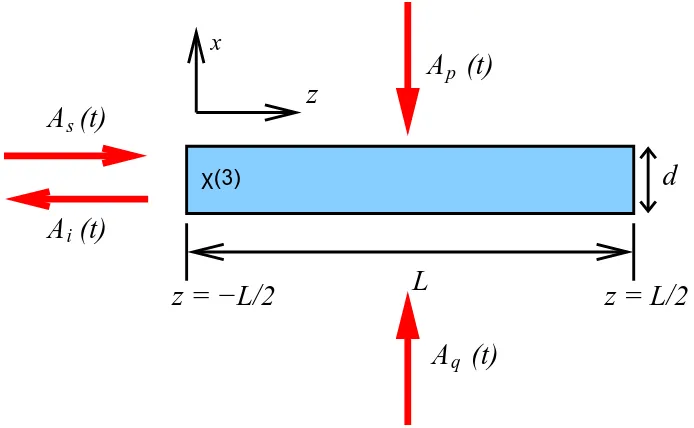
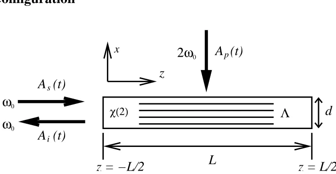
Figure 4.1: Setup of SPC by four-wave mixing. As(t)is the signal pulse, Ap(t)and Aq(t)are the pump pulses, and Ai(t)is the backward-propagating idler pulse. (After Ref. [1])

[image:35.612.152.499.153.367.2]

The configuration of spectral phase conjugation by four-wave mixing introduced in Ref. [1] is drawn in Fig. 4.1. Apand Aqare the envelopes of the pump pulses propagating downward and upward, respectively. As is the forward-propagating signal envelope; and Aiis the backward-propagating idler envelope. The coupled-mode equations that govern Ap, Aq, Asand Aican be derived from the wave equation and are given by

−∂_∂Ap

x +

1

vx

∂Ap

∂t = jγ[2AsAiA

∗

q+ (|Ap|2+2|Aq|2+2|As|2+2|Ai|2)Ap], (4.1)

∂Aq

∂x +

1

vx

∂Aq

∂t = jγ[2AsAiA

∗

p+ (2|Ap|2+|Aq|2+2|As|2+2|Ai|2)Aq], (4.2)

∂As

∂z +

1

v

∂As

∂t = jγ[2ApAqA

∗

i+ (2|Ap|2+2|Aq|2+|As|2+2|Ai|2)As], (4.3) −∂_∂A_zi+1

v

∂Ai

∂t = jγ[2ApAqA

∗

s+ (2|Ap|2+2|Aq|2+2|As|2+|Ai|2)Ai], (4.4)

γ = 3ω0χ

(3)

8cn0

, (4.5)

(36)

be neglected.

The zeroth-order solution is the linear propagation of the incoming waves. Let the zeroth-order solution be

A(p0)(x,t) = Ap(t), (4.6)

A(q0)(x,t) = Aq(t), (4.7)

A(s0)(z,t) = F(t−

z

v), (4.8)

A(_i0)(z,t) = 0. (4.9)

The first-order solution can then be obtained by substituting the zeroth-order solution into the right-hand side of Eqs. (4.3) and (4.4). Each of Eqs. (4.1)₋(4.4) has a single wave mixing term (first term on the right-hand side) and four phase modulation terms, which generally distort the pulses. With the subsitutions only Eq. (4.4) has a nonzero wave mixing term, and the output idler Ai(−L₂,t)in the first order is shown to be the SPC of the input signal [1],

A(_i1)(−L₂,t) = jF∗(−t+ L

2v) Z ∞

−∞

2γvAp(t′)Aq(t′)dt′, (4.10)

and the conversion efficiency is

η(1)

≡ R∞

−∞|A

(1)

i (− L 2,t′)|2dt′ R∞

−∞|A(s1)(−L₂,t′)|2dt′

= [ Z ∞

−∞|2γvAp(t ′₎_A

q(t′)|dt′]2, (4.11)

assuming that either of the pump pulses Apand Aqis much shorter than the input signal F and the medium is long enough to contain the signal. Conceptually, the short pump pulses take a “snapshot” of the signal spatial profile, which is reproduced as the idler. Since the idler has the same spatial profile as the signal but propagates backwards, the time profile is reversed.

To summarize, in order to perform accurate SPC, the following conditions should be satisfied:

L

v >>Ts>>(Tpor Tq)>> d vx

, (4.12)

where Tsis the signal pulse width, and Tpand Tqare the pulse widths of the two pumps.

4.3

High conversion efficiency with signal amplification

(37)

and undepleted, and phase modulation terms are neglected, we can derive a closed-form solution for the conversion efficiency. Eqs. (4.3) and (4.4) then become

v∂As(z,t)

∂z +

∂As(z,t)

∂t = jg(t)A

∗

i(z,t), (4.13)

−v∂Ai(z,t)

∂z +

∂Ai(z,t)

∂t = jg(t)A

∗

s(z,t), (4.14)

where g(t) = 2γvAp(t)Aq(t). (4.15)

We first take the complex conjugate of Eq. (4.14),

−v∂A∗i(z,t)

∂z +

∂A∗_i(z,t)

∂t =−jg

∗₍_t₎_A

s(z,t), (4.16)

and let ˜Asand ˜Aibe the Fourier transforms of Asand A∗i with respect to z, respectively,

˜

As(κ,t) = Z ∞

−∞

As(z,t)exp(−jκz)dz, (4.17) ˜

Ai(κ,t) = Z ∞

−∞A ∗

i(z,t)exp(−jκz)dz. (4.18) Note that ˜Aiis the Fourier transform of the complex conjugate of Ai. Eqs. (4.13) and (4.16) become

jκv ˜As+∂ ˜

As

∂t = jg(t)A˜i, (4.19)

−jκv ˜Ai+

∂_A˜_i

∂t = −jg

∗₍_t₎_A˜

s. (4.20)

We multiply both sides of Eq. (4.19) by exp(jκvt)and both sides of Eq. (4.20) by exp(−jκvt),

exp(jκvt)(jκv ˜As+∂ ˜

As

∂t ) = jg(t)exp(jκvt)

˜

Ai, (4.21)

exp(−jκvt)(−jκv ˜Ai+

∂_A˜_i

∂t ) = −jg

∗₍_t₎_exp₍₋_j_κ_vt₎_A˜

s, (4.22)

or equivalently,

∂

∂t[exp(jκvt)

˜

As] = jg(t)exp(jκvt)A˜i, (4.23)

∂

∂t[exp(−jκvt)A˜i] = −jg

∗₍_t₎_exp₍₋_j_κ_vt₎_A˜_s_. _(4.24)

Then we make another set of substitutions,

A(κ,t) = exp(jκvt)A˜s=exp(jκvt) Z ∞

−∞As(z,t)exp(−jκz)dz, (4.25)

B(κ,t) = exp(−jκvt)_A˜_i₌_exp₍₋_j_κ_vt₎Z ∞

−∞

(38)

Eqs. (4.23) and (4.24) become

∂A

∂t = jg(t)exp(2 jκvt)B, (4.27)

∂B

∂t = −jg

∗₍_t₎_exp₍₋_{2 j}_κ_vt₎_A_. _(4.28)

The exponential terms on the right-hand side have a frequency 2κv. To estimate the magnitude of this

frequency, it is best to first consider the linear propagation of the signal and idler envelopes, before wave mixing occurs,

v∂As

∂z +

∂As

∂t = 0, (4.29)

−v∂Ai

∂z +

∂Ai

∂t = 0. (4.30)

Fourier transforms in z as well as t give the dispersion relation for the envelopes,

|κv_|=|Ω|, (4.31)

which is consistent with the definition of group velocity, v= d_dkω. Ω is the frequency variable in taking the temporal Fourier transform of the signal and idler envelopes, and has a maximum magnitude_∼1/Ts. From Eqs. (4.27) and (4.28) it can be observed that wave mixing does not alter the spatial bandwidth of the envelopes, thereforeκhas the same order of magnitude throughout, andκv_∼1/Ts<<(1/Tpor 1/Tq). g(t) has a duration shorter than both Tpand Tq, so exp(2 jκvt)oscillates relatively slowly compared to g(t). Say

g(t)is centered at t=0, we can then make the assumption

g(t)exp(2 jκvt)≈g(t). (4.32)

The coupled-mode equations (4.27) and (4.28) become

∂A

∂t = jg(t)B, (4.33)

∂B

∂t = −jg

∗₍_t₎_A_. _(4.34)

The initial condition is

As(z,−

L

2v) = F(−

L

2v−

z

v), (4.35)

Ai(z,−

L

(39)

The initial condition for A and B can then be obtained from the substitutions, Eqs. (4.25) and (4.26). Define

g(t) =|g(t)|exp jθ(t), and assume thatθ(t)is a constant. Eqs. (4.33) and (4.34) can now be solved to give

A(κ,t) = A(κ,−_2vL)cosh[ Z t

−L

2v

|g(t′)|dt′], (4.37)

B(κ,t) = −jA(κ,−_2vL)exp(−jθ)sinh[ Z t

−2vL

|g(t′)|dt′]. (4.38)

The final solution for Asand Aiis

As(z,t) = F(t−

z v)cosh[

Z t

−L

2v

|g(t′)|dt′], (4.39)

Ai(z,t) = jF∗(−t−

z

v)exp(jθ)sinh[

Z t

−L

2v

|g(t′)|dt′]. (4.40)

As the idler exits the medium at z=−L 2and t=

L

2v, the pump pulses have long gone, hence the upper integral limit can be effectively replaced by∞. The lower limit can also be replaced by₋∞, since the pump pulses have not arrived when the signal enters the medium at t=−L

2v. Hence

Ai(−

L

2,t) =jF

∗₍₋_t₊ L

2v)exp(jθ)sinh[ Z ∞

−∞|g(t

′₎_|_dt′_]_. _(4.41)

This solution is consistent with Eq. (4.10), the first-order approximation in the limit of small gain. The conversion efficiency is

η≡

R∞

−∞|Ai(−₂L,t′)|2dt′ R∞

−∞|As(−₂L,t′)|2dt′

=sinh2[ Z ∞

−∞|

2γvAp(t′)Aq(t′)|dt′]. (4.42)

This result shows the exponential dependence of the conversion efficiency on the cross fluence of the two pump pulses.

4.4

Cross-phase modulation compensation

(40)

With XPM terms included, the coupled-mode equations become

v∂As(z,t)

∂z +

∂As(z,t)

∂t = jg(t)A

∗

i(z,t) +jc(t)As(z,t), (4.43) −v∂Ai(z,t)

∂z +

∂Ai(z,t)

∂t = jg(t)A

∗

s(z,t) +jc(t)Ai(z,t), (4.44) where g(t) = 2γvAp(t)Aq(t), (4.45)

c(t) = 2γv

|Ap(t)|2+|Aq(t)|2. (4.46)

XPM effects are detrimental to the SPC efficiency and accuracy if a high conversion efficiency is desired, as it introduces a time-dependent detuning factor to the wave mixing process.

To solve Eqs. (4.43) and (4.44), we follow similar procedures as in the previous section by performing a Fourier transform with respect to z and making the following substitutions:

A(κ,t) = exp[jκvt₋j

Z t

−∞c(t

′₎_dt′_]Z ∞

−∞As(z,t)exp(−jκz)dz, (4.47)

B(κ,t) = exp[−jκvt+j

Z t

−∞c(t

′₎_dt′_]Z ∞ −∞A

∗

i(z,t)exp(−jκz)dz. (4.48) We obtain the following:

∂A

∂t = jg(t)exp[−2 j

Z t

−∞

c(t′)dt′]B, (4.49)

∂B

∂t = −jg

∗₍_t₎_exp_[_{2 j}Z t −∞

c(t′)dt′]A. (4.50)

Eqs. (4.49) and (4.50) are difficult to solve analytically, but a special case exists when the phase of g(t)

exactly cancels the XPM term,

θ(t) = θ0+2 Z t

−∞c(t

′₎_dt′_. _(4.51)

Eqs. (4.49) and (4.50) are then reduced to

∂A

∂t = j|g(t)|exp(jθ0)B, (4.52)

∂B

∂t = −j|g(t)|exp(−jθ0)A. (4.53)

The general solution is

As(z,t) = F(t−

z v)exp[j

Z t

−∞c(t

′₎_dt′_]_cosh_[Z t −∞|g(t

′₎_|_dt′_]_, _(4.54)

Ai(z,t) = jF∗(−t−

z

v)exp[jθ0+j

Z t

−∞c(t

′₎_dt′_]_sinh_[Z t −∞|g(t

(41)

and the output idler is

Ai(−

L

2,t) =jF

∗₍₋_t₊ L

2v)exp[jθ0+j Z ∞

−∞c(t

′₎_dt′_]_sinh_[Z ∞ −∞|g(t

′₎_|_dt′_]_. _(4.56)

This solution is the same as Eq. (4.41), the output idler without considering XPM, apart from a constant phase term exp[R∞

−∞c(t′)dt′], which does not affect the pulse waveform. If we let Ap(t) =|Ap(t)|exp[jθp(t)]and

Aq(t) =|Aq(t)|exp[jθq(t)], then from Eq. (4.51) the actual phase adjustments to the pump pulses are given by

θp(t) +θq(t) =θ0+4γv Z t

−∞|

Ap(t′)|2+|Aq(t′)|2dt′. (4.57)

Qualitatively, by adjusting the phases of the pump pulses according to Eq. (4.57), we can utilize the wave mixing process to introduce phase variations to the signal and the idler, so that the cross-phase modulation can be exactly canceled. In practice, the phase variation of the pump pulses can be introduced by various pulse shaping methods, for example, using a 4f pulse shaper [12]. The phase correction can be introduced to either or both of the pump pulses as long as the condition in Eq. (4.57) is satisfied.

4.5

Numerical analysis

To verify our derivations, we obtain numerical solutions of Eqs. (4.43) and (4.44) by a multiscale approach. In this approach successively higher-order solutions are obtained by substituting lower-order solutions into the right-hand side of the equations, until convergence is reached. For the following simulations, the pump and the input signal are assumed to be

Ap(t) =Aq(t) = exp −

t2

2T2 p

, (4.58)

F(τ) = As0

n

exp₋1+j 2 (

τ+2Ts

Ts

)2] +1

2exp

−1₂(τ−2Ts

Ts

)2o

. (4.59)

(42)

−10 −5 0 5 10 0

0.5 1 1.5

time (ps)

intensity (a.u.)

(a) Intensity at z = −L/2

−10 −5 0 5 10

−3 −2 −1 0 1 2 3

time (ps)

phase (radian)

(b) Phase at z = −L/2

Idler Signal

[image:42.612.174.476.234.483.2]

Idler Signal

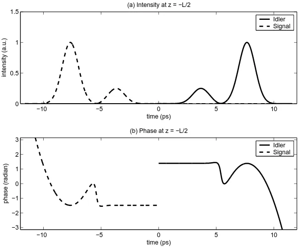
Figure 4.2: (a) Amplitude and (b) phase of output idler (solid lines) Ai(−L2,t)compared with input signal (dash lines) As(−L₂,t). XPM is neglected in this example. As predicted, the output idler is time-reversed and phase-conjugated with respect to the input signal. Parameters used are n2=1×10−11cm2/W, n0=1.7,

λ0=800 nm, L=2 mm, d=5µm, Ts = 1 ps, Tp= 100 fs, Ep= 12.8 nJ, pump fluence = Ep

(43)

4.5.1

Conversion efficiency

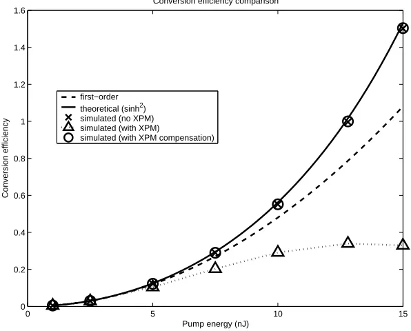
Figure 4.3 is a plot of conversion efficiencies against total pump energy obtained from theory and simulations, using the same parameters as for the previous numerical example. The dotted curve is a plot of Eq. (4.11), the result from Ref. [1]. The solid curve is a plot of Eq. (4.42), the conversion efficiency obtained by including signal amplification but neglecting XPM. The crosses are results from a numerical simulation of Eqs. (4.13) and (4.14), validating the closed-form solution we derive. The triangles are results from a numerical simula-tion of Eqs. (4.3) and (4.4), which also include phase modulasimula-tion terms. It clearly shows that XPM becomes detrimental to the conversion efficiency as the pump energy increases. Finally, the circles are a numerical simulation that includes all nonlinear terms and XPM compensation according to Eq. (4.57). The numerical results confirm the accuracy of our conversion efficiency derivation, demonstrates the detrimental XPM effect on conversion efficiency, and proves that our compensation method can indeed undo the XPM effect.

0 5 10 15

0 0.2 0.4 0.6 0.8 1 1.2 1.4 1.6

Conversion efficiency comparison

Pump energy (nJ)

Conversion efficiency

first−order theoretical (sinh2) simulated (no XPM) simulated (with XPM)

[image:43.612.174.472.289.529.2]

simulated (with XPM compensation)

Figure 4.3: Conversion efficiencies from simulations compared with predictions from first-order analysis and coupled-mode theory. Simulation results agree well with coupled-mode theory. See caption of Fig. 4.2 for parameters used.

4.5.2

Demonstration of cross-phase modulation compensation

(44)

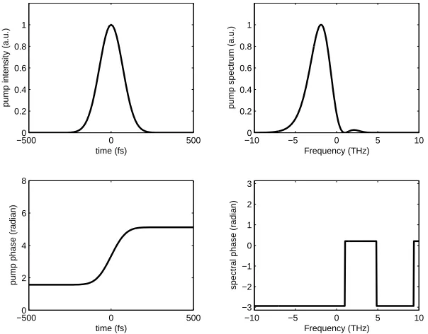
2 4 6 8 10 0 0.5 1 1.5 time (ps) intensity (a.u.)

(a) Intensity at z = −L/2

2 4 6 8 10

−3 −2 −1 0 1 2 3 time (ps) phase (radian)

(b) Phase at z = −L/2

2 4 6 8 10

0 0.5 1 1.5 time (ps) intensity (a.u.)

(c) Intensity at z = −L/2

2 4 6 8 10

−3 −2 −1 0 1 2 3 time (ps) phase (radian)

(d) Phase at z = −L/2 Idler SPC of Signal

Idler SPC of Signal Idler

SPC of Signal

[image:44.612.175.475.77.327.2]

Idler SPC of Signal

Figure 4.4: (a) and (b) plot the normalized amplitude and phase of the output idler Ai(−L₂,t)compared to the SPC of the input signal A∗_s(−L

2,−t), respectively, when XPM is present. The amplitude plots are normalized with respect to their peaks. The output idler is distorted and the conversion efficiency is only 34%, much lower than the theoretical efficiency 100%. (c) and (d) plot the same data, but with XPM compensation. The efficiency is back to 100% and the accuracy is restored.

−5000 0 500

0.2 0.4 0.6 0.8 1 time (fs)

pump intensity (a.u.)

−5000 0 500

2 4 6 8

time (fs)

pump phase (radian)

−100 −5 0 5 10

0.2 0.4 0.6 0.8 1 Frequency (THz)

pump spectrum (a.u.)

−10 −5 0 5 10

−3 −2 −1 0 1 2 3 Frequency (THz)

spectral phase (radian)

[image:44.612.174.476.418.654.2]

(45)

4.6

Beyond the basic assumptions

4.6.1

Pump depletion

All of our derivations so far assume that the pump is undepleted. If the signal becomes comparable to the pump, then the pump can no longer sustain a fixed gain, which begins to depend on the signal field across

z. Mathematically this means that the right-hand sides of Eqs. (4.1) and (4.2) become comparable to the

left-hand sides. In this case the pump would be depleted, and we can no longer expect the SPC operation to be accurate. To avoid pump depletion we therefore require the right-hand sides of Eqs. (4.1) and (4.2) to be much smaller than the left-hand sides, or roughly speaking,

|A_p| >> 2γ_|A_s||A_i||A_q|d, (4.60)

Es <<

n0dTs

η0γ√η

. (4.61)

where Esis the signal energy andη0is the free-space impedance. The signal energies should be much smaller than the rough signal energy upper limits established by Eq. (4.61) in order to avoid pump depletion. A low signal energy also avoids distortion due to SPM.

To investigate the effect of pump depletion, we perform three-dimensional simulations in x, z, t by nu-merically solving Eqs. (4.1), (4.2), (4.3), and (4.4) simultaneously.

The first example assumes the same parameters as before, with a signal energy of 1 pJ, much below the pump depletion limit, calculated to be 1 nJ from Eq. (4.61). XPM is included along with XPM compensa-tion. The conversion efficiency from the simulation drops slightly to 92% due to a finite medium thickness. However, the SPC process still remains accurate with the inclusion of the x dimension.

On the other hand, with a signal energy of 5 nJ, much above the pump depletion limit 1 nJ, Fig. 4.6 plots the output idler from the same simulation. As can be seen from the movie, the pump pulses are highly depleted, and from Fig. 4.6 it can be seen that the top of the idler is flattened due to gain saturation. The conversion efficiency is reduced to 32%.

4.6.2

Other nonideal conditions

Besides pump depletion, other nonideal conditions also affect the accuracy of the SPC process. If the pump pulses are not short enough, then from the first-order solution in Ref. [1] it can be seen that the output pulse becomes the convol