City, University of London Institutional Repository
Citation
:
Cowell, R., Lauritzen, S. L. and Mortera, J. (2006). Identification and separation of DNA mixtures using peak area information (Updated version of Statistical Research Paper No. 25) (Statistical Research Paper No. 27). London, UK: Faculty of Actuarial Science & Insurance, City University London.This is the unspecified version of the paper.
This version of the publication may differ from the final published
version.
Permanent repository link:
http://openaccess.city.ac.uk/2371/Link to published version
:
Statistical Research Paper No. 27Copyright and reuse:
City Research Online aims to make research
outputs of City, University of London available to a wider audience.
Copyright and Moral Rights remain with the author(s) and/or copyright
holders. URLs from City Research Online may be freely distributed and
linked to.
City Research Online: http://openaccess.city.ac.uk/ [email protected]
Faculty of Actuarial
Science
and
Statistics
Identification and
Separation of DNA Mixtures
Using Peak Area
Information.
(Updated Version of Statistical Research Paper
No. 25)
R.G. Cowell, S.L. Lauritzen and J. Mortera.
Statistical
Research Paper No. 27
February 2006
ISBN 1-901615-94-4
Cass Business School 106 Bunhill Row London EC1Y 8TZ
T +44 (0)20 7040 8470
Identification and Separation of DNA Mixtures using
Peak Area Information
R. G. Cowell
∗Faculty of Actuarial Science and Statistics,
Cass Business School,
106 Bunhill Row,
London EC1Y 8TZ, UK.
S. L. Lauritzen
Department of Statistics,
University of Oxford
1 South Parks Road,
Oxford OX1 3TG, U.K.
J. Mortera
Dipartimento di Economia
Universit`a Roma Tre
Via Ostiense, 139
00154 Roma, Italy
February 14, 2006
THIS IS AN UPDATED VERSION OF RESEARCH REPORT 25
SIR JOHN CASS BUSINESS SCHOOL CITY UNIVERSITY
Abstract
We introduce a new methodology, based upon probabilistic expert systems, for analysing forensic identification problems involving DNA mixture traces using quan-titative peak area information. Peak area is modelled with conditional Gaussian distributions. The expert system can be used for ascertaining whether individuals, whose profiles have been measured, have contributed to the mixture, but also to predict DNA profiles of unknown contributors by separating the mixture into its in-dividual components. The potential of our probabilistic methodology is illustrated on case data examples and compared with alternative approaches. The advantages are that identification and separation issues can be handled in a unified way within a single probabilistic model and the uncertainty associated with the analysis is quan-tified. Further work, required to bring the methodology to a point where it could be applied to the routine analysis of casework, is discussed.
Some key words and phrases: DNA mixture, forensic identification, mixture separa-tion, probabilistic expert system, peak weight.
1
Introduction
Probabilistic expert systems (PES) for evaluating DNA evidence were introduced by Dawid et al. [1]. In a general review of the analysis of DNA evidence, Foreman et al. [2] include several applications of PES and emphasize their potential by predicting that this method-ology “will offer solutions to DNA mixtures and many more complex problems in the future.”.
This article is concerned with the analysis ofmixed traceswhere several individuals may have contributed to a DNA sample left at a scene of crime. Mortera et al. [3] showed how to construct a PES using information about which alleles were present in the mixture, and we refer to this article for a general description of the problem and for genetic background information. Other earlier contributions based solely on allelic presence in the mixture are Evett et al. [4] and Weir et al. [5].
The results of a DNA analysis are usually represented as an electropherogram (EPG) measuring responses in relative fluorescence units (RFU) and the alleles in the mixture correspond to peaks with a given height and area around each allele, see Figure 1. The band intensity around each allele in the relative fluorescence units represented, for example, through their peak areas, contains important information about the composition of the mixture.
Figure 1: An electropherogram (EPG) of marker VWA from a mixture. Peaks represent alleles at 15, 17 and 18 and the areas and height of the peaks express the quantities of each. Since the peak around 17 is high, this indicates two alleles with repeat number 17. This image is supplied courtesy of LGC Limited, 2004.
More recently, Bill et al. [8] have developed PENDULUM, a computer package to automate the guidelines in [6] and [7]. First, a list of all possible genotype combinations is made and those outside heterozygous peak balance limits are eliminated; then the list is scored with respect to mixture proportion. The possibility of allelic dropout is considered, but other artifacts, such as stutter, are not accounted for. The primary purpose of PENDULUM is to eliminate unreasonable genotypic combinations. It also ranks the genotypes but this is not based on a probabilistic order, so no quantification of the uncertainty in the analysis is possible. Evidential calculations cannot be carried out directly within PENDULUM, however they may be performed by using the output of PENDULUM as the input to an external probabilistic model.
The methods utilizing peak area information described above are not probabilistic in nature, nor do they use information about allele frequency. In contrast, the methodology proposed in Evett et al. [11] combines a model using the gene frequencies with a model describing variability in scaled peak areas to calculate likelihood ratios and study their sensitivity to assumptions about the mixture proportions.
Our approach incorporates elements similar to all of those described above, but unifies these in a single Bayesian network model. More specifically, we build a PES for mixture traces based on conditional Gaussian distributions for the peak areas, given the compo-sition of the true DNA mixtures; see Chapter 7 of [12] as well as [13]. The exact same network is then used both for an evidential calculation as well as for the separation of DNA mixtures, with the additional benefit of a full probabilistic quantification of any uncertainty associated with the analysis.
The main focus of the present paper is to illustrate the basic ideas in a new methodology for resolving DNA mixtures based on PES. For the sake of clarity and simplicity, we only consider a DNA mixture from exactly two contributors, which seems to be the most common scenario in forensic casework [14]. We do not allow for further complications such as stutter, dropout alleles, etc. In order to develop the methodology into a practical tool for forensic laboratories these additional complications will need to be considered. However, we emphasize that the flexibility and modularity of the PES approach readily enables extension and modification of our network to include complications such as an unknown number of contributors, indirect evidence, dropout, stutter, etc. along the lines given in [3].
An analysis of a mixed trace can have different purposes, several of which can be relevant simultaneously, making a unified approach particularly suitable. However, for the sake of exposition we consider the issues separately. The first focus of our analysis will be that of evidential calculation, detailed in §4. Here a suspect with known genotype is held and we want to determine the likelihood ratio for the hypothesis that the suspect has contributed to the mixture vs. the hypothesis that the contributor is a randomly chosen individual. We distinguish two cases: the other contributor could be avictim with a known genotype or a contaminator with an unknown genotype, possibly without a direct relation to the crime. This could be a laboratory contamination or any other source of contamination from an unknown contributor.
Another use of our network is the separation of profiles, i.e. identifying the genotype of each of the possibly unknown contributors to the mixture, the evidential calculation playing a secondary role. This use is illustrated in §5.
2
Basic model assumptions
taken from Clayton et al. [6], Perlin and Szabady [9]1 and Wang et al. [10].
We first present a description of the model before introducing the mathematical details. In essence, the PES is a probabilistic model for relating the pre-amplification and post-amplification relative amounts of DNA in a mixture sample. The model is idealized in that it ignores complicating artifacts such as stutter, drop-out alleles and so on, and assumes that the mixture is made up of DNA from two people, who we refer to as p1 and p2. Now prior to amplification, and provided the mixture sample has not been degraded to the point of breaking up tissue cells, the sample put into the amplification apparatus will consist of an unknown number of cells from p1 and a further unknown number of cells from p2. Then, with every cell containing exactly two alleles from each marker, the fraction or proportion of cells from p1 is also a common measure across the markers of the amount of DNA from p1. We denote this common fraction, or proportion, by θ.
In an ideal amplification apparatus, during each amplification cycle the proportion of alleles of each allelic type would be preserved without error. We model departures from this ideal as random variation using the Gaussian distributions in (1), whose mean for each allele is its pre-amplification proportion for the marker system it belongs to. The variance has a simple dependence on the mean such that in the two limiting cases of (i) the pre-amplification proportion is zero, or (ii) the pre-amplification proportion is unity, the variance is zero. In the case of (i) this means that if there is no allele of a certain type in the mixture prior to amplification, there is none post-amplification. In the case of (ii) this means that if for a given marker there is only one allelic type present in the mixture pre-amplification, then only that type is present in that marker post-amplification. Our model introduces an additional variance term to represent other measurement error, represented by ω2.
The post-amplification proportions of alleles for each marker are represented in the peak area information, which we include in the analysis through the relative peak weight. The (absolute) peak weight wa of an allele with repeat number a is defined by scaling the
peak area with the repeat number as
wa=aαa,
where αa is the peak area around allele a. Multiplying the area with the repeat number
is a crude way of correcting for the fact that alleles with a high repeat number tend to be less amplified than alleles with a low repeat number. For issues concerning heterozygous imbalance see [16].
We further assume that
• The pre-amplification mixture proportionθis constant across markers, for the reasons outlined above;
• The peak weight for an allele possessed by both contributors is the sum of the cor-responding weights for the two contributors.
To avoid arbitrariness in scaling we consider the observed relative peak weight ra,
ob-tained by scaling with the total peak weight as
ra=wa/w+, w+ =
X
a
wa,
so that then P
ara= 1.
Our simple model for the relative peak weight, denoted by the random variable Ra,
assumes a Gaussian error distribution
Ra∼ N(µa, τa2), µa={θn(1)a + (1−θ)n(2)a }/2, (1)
where θ is the proportion, or fraction, of DNA in the mixture originating from the first contributor, n(i)
a is the number of alleles with repeat number a possessed by person i.
The error variance τ2
a has the form
τa2 =σ2µa(1−µa) +ω2 (2)
where σ2 and ω2 are variance factors for the contributions to the variation from the
am-plification and measurement processes.
The model can be seen as a second order approximation to a more sophisticated model based on gamma distributions for the absolute scaled peak weights (to be discussed else-where).
In addition we need to consider the correlation between weights due to the fact that they must add up to unity. If this is the only source of correlation, its inferential effect can be taken correctly into account by using the variance structure
τa2 =σ2µa+ω2 (3)
and considering the complete set of observed peak weights as observed evidence, as argued in Appendix A. Note that this is in contrast to Cowell et al. [17] who ignored the correlation without modifying the variance from (2) to (3), but essentially obtained results with the same qualititative behaviour as in the present paper.
Unless stated otherwise, we have used σ2 = 0.01 and ω2 = 0.001, corresponding
ap-proximately to a standard deviation for the observed relative weight of about
q
0.01/4 + 0.001 = 0.06
for µa = 0.5 substituted into (2). These parameter values imply that when amplifying
DNA from one heterozygous individual (for which µa = 0.5), an ra value at two standard
been reported in the literature [18], and suggests that our chosen parameter values are perhaps conservative.
In general the variance factors may depend on the marker and on the amount of DNA analysed, but for simplicity we use the values above. Our PES model is robust to small changes in these parameter estimates. We are planning a full data analysis in order to refine the estimates and obtain a proper calibration of the variances for use in casework.
The simple model above seems in any case sufficiently accurate and adequate for the purposes of the present paper, and has the advantage that the calculations may be per-formed quickly using any available Bayesian network software that implements evidence propagation for conditional-Gaussian networks.
3
Bayesian networks for DNA mixtures with peak
weights
3.1
Background
Here we give a very brief description of the basic ingredients of a Bayesian network or probabilistic expert system. Complete details can be found in [12]. A Bayesian network represents, by means of a directed acyclic graph (DAG), the complex probabilistic rela-tionships of dependence and independence among a set of variables. (See Figure 11 for a simple example.) The nodes of the network represent the random variables and directed edges (arrows) connecting nodes describe the relationships among the variables. The joint probability structure of all the nodes in the network is determined by the conditional prob-ability of each node given its graphical “parents”2. The joint probability model of all the
nodes is thus expressed in terms of simple submodels. Fast and efficient computational algorithms exist for the exact calculation of marginal and conditional probabilities for the conditional-Gaussian networks used in this paper [13]. These enable the evidence (or in-formation) on a set of nodes to be propagated to all nodes in the network and thus obtain the updated posterior conditional probabilities for all the variables represented.
Bayesian networks can easily be implemented using readily available software such
as Hugin3. The graphical interface can be used to specify the qualitative relationships
between the variables, their values and the conditional probabilities. The network is then compiled (giving the marginal distribution of all nodes) and after evidence is inserted and propagated throughout the network the updated conditional probability distributions can be read off the nodes of interest.
The Bayesian networks constructed for the examples in this paper were implemented
in Hugin, as described in Appendix B, and also in a separate programMaies, described
high level of discretization were initially performed using Maies, and then checked using
Hugin by exporting from Maies non object-oriented Bayesian networks to files in the
Hugin format.
3.2
Object-Oriented Networks
Object-oriented Bayesian networks [19, 20] have a hierarchical structure where any node itself can represent a (object-oriented) network containing severalinstancesof other generic classes of networks. This framework is particularly suited for an application area such as the present because we can exploit the similarity between elements of the networks in a modular and flexible construction, making the networks more and more complex by simply adding new objects which perform different tasks. Two recent examples of object-oriented Bayesian networks applied to forensic DNA problems are [21] and [22].
Instances have interface input and output nodes as well as ordinary nodes. Instances of a particular class have identical conditional probability tables for non-input nodes. In-stances are connected by arrows from output nodes to input nodes. These arrows represent identity links whereas arrows between ordinary nodes represent probabilistic dependence. Implementation of object-oriented Bayesian networks is supported by the programHugin
6.4, which we use in our analyses. A more detailed description of the component object-oriented networks used in this paper may be found in Appendix B.
3.3
Maies: A PES for analysing mixed traces
As indicated above, in parallel to the development of the object-oriented networks a sep-arate computer program called Maies—Mixture Analysis In Expert Systems—was
de-veloped to provide an independent check of the calculations. It also provided a flexible environment for specification of input and output of data that allowed for sensitivity anal-ysis and, for example, to provide the data in a useful form for producing posteriors plots.
The input toMaies is simply the measured peak area information on up to four alleles
per marker, the population gene frequencies of these alleles, and additional genotypic information (if available) about the potential contributors.
After entering peak area information and available genetic profiles on people, the soft-ware constructs a single Bayesian network on which the probability calculations are per-formed (see Figure 20). In constructing the Bayesian network the user is presented with the options of changing default values for the scale σ2 of the amplification error variance,
the measurement error variance ω2, and the number of discrete states used for the node
that represents θ, the true pre-amplification fraction of DNA originating from individual 1. Sensitivity analysis may be performed in a simple, straightforward manner by varying these three inputs. Peak areas are automatically converted to normalized weights by the program, and entered as evidence in the relevant nodes.
vice versa. A more detailed description of the networks generated byMaies may be found
in Appendix C.
4
Evidence calculations
This section illustrates (through the analysis of real mixture examples) how to use our PES to calculate the weight of the evidence—in the form of a likelihood ratio—for a given suspect to have contributed to a trace under different circumstances.
The evidence could consist of DNA profiles extracted from asuspect, s, avictim, v,and the mixed trace. In this case we compute the likelihood ratio in favour of the hypothesis that the victim and suspect contributed to the mixture: H0 :v&s, vs. the hypothesis that
the victim and an unknown individual, u contributed to the mixture: H1 :v&u.
A variant has an unknown contaminator, u instead of a victim, in which case the hypotheses are H0 :u&s versus H1 : 2u.
In the results shown below (and also for the examples in §5) the variable describing the mixture proportionθ has been discretized to having 101 states 0,0.01,0.02, . . . ,0.99,1, but experiments indicate very low sensitivity to the discretization as long as it is not far too rough and 10-20 states would probably be fully appropriate.
4.1
Genotype of suspect and victim available
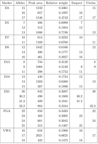
This example is taken from Wang et al. [10], stating P. Graham of the Texas Department of Public Safety as the data source. Table 1 displays the alleles observed in the mixture, the measured peak area and the relative weight on 9 markers, together with the genotypes of two potential contributors, here named suspect, s and victim,v. We will in the following refer to this data as the Grahamdata.
The evidence in this table is now entered and propagated throughout the network yielding the marginal posterior probabilities or densities of the quantities of interest. The evidence on allelic repeat number is inserted in the appropriate nodes; details on how this is done are given in Appendix B.6 and Appendix C.4. When peak area information is also used, the nodes representing the observed relative peak weights are set to their correspond-ing values, as illustrated in Appendix B.7 and Appendix C.5. Takcorrespond-ing appropriate ratios in the posterior probabilities associated with the target node yields the likelihood ratio in favour of H0 : v&s versus H1 : v&u. Table 2, column “Areas” displays the logarithm
of this likelihood ratio, and column “Alleles” the corresponding ratio when only the evi-dence on the repeat number of the alleles is used. The last columns of Table 2 show the log-likelihood ratio when the mixture proportion θ is assumed known at given values. The same network is used to compute all the quantities in Table 2.
Table 1: Grahamdata showing mixture composition, peak areas, relative weights, suspect’s and victim’s profiles.
Marker Alleles Peak area Relative weight Suspect Victim
D3 15 1242 0.3361 15
16 657 0.1897 16
17 1546 0.4742 17 17
D5 7 486 0.0999 7
12 512 0.1804 12
13 1886 0.7198 13
D7 10 614 0.3232 10
11 1169 0.6768 11
D8 12 1842 0.6166 12
13 490 0.1777 13
16 461 0.2057 16
D13 8 734 0.3128 8
9 1068 0.5120 9 9
11 299 0.1752 11
D18 12 440 0.1724 12
13 1503 0.6380 13
15 387 0.1896 15
D21 30 842 0.3087 30
30.2 490 0.1808 30.2
31.2 509 0.1941 31.2
32.2 804 0.3164 32.2
FGA 22 850 0.3483 22
23 468 0.2005 23
24 681 0.3045 24
25 315 0.1467 25
VWA 16 616 0.1900 16
17 2021 0.6625 17
Table 2: Logarithm of the likelihood ratios in favour of H0 :v&s vs. H1 :v&u
for the Grahamdata.
Areas Alleles Assumed known mixture proportion
θ 0.1 0.2 0.3 0.4 0.5 0.6 0.7 0.8 0.9
Log10LR 14.47 12.93 10.97 13.44 14.46 14.42 12.42 8.58 2.76 -7.19 -27.79
0.20 0.25 0.30 0.35 0.40 0.45 0.50
0.00
0.05
0.10
0.15
0.20
Proportion of DNA from suspect
[image:14.595.146.450.415.613.2]Posterior density
The inclusion of area information is indeed strengthening the evidence against the suspect, increasing the logarithm of the likelihood ratio from 12.93 to 14.47, approximately corresponding to a factor 36. This is a modest increase and reflects the fact that when information about the genotype of the victim is available, peak area does not make much difference to the likelihood ratio as the genotypes themselves are very informative.
4.2
Only genotype of suspect available
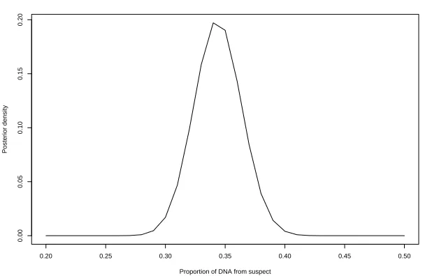
Our next example is taken from Evett et al. [11] and has only information of the geno-type from one potential contributor, here named the suspect, whereas the other unknown contributor is termed contaminator. The data refers to a 10:1 mixture of two individuals. The data is displayed in Table 3 and is henceforth referred to as the Evett data. Table 4 displays the logarithm of this likelihood ratio together with the corresponding ratio when peak weights are ignored, and the ratios when the mixture proportion θ is assumed known at given values.
Note that the strengthening of evidence against the suspect is more dramatic when information on the contaminator is absent: the logarithm of the likelihood ratio changes from 4.4 to 8.23, corresponding to an additional factor around 6000, as compared to a factor 36 above.
Also here the likelihood ratio is essentially constant over a region which completely covers the posterior plausible range 0.85< θ <0.95.
The posterior distribution of the mixture proportion θ is displayed in Figure 3. The maximum occurs around the value 0.90 which is a little off the true 10:1 mixture proportion.
0.80 0.85 0.90 0.95 1.00
0.00
0.05
0.10
0.15
Proportion of DNA from suspect
[image:15.595.146.450.474.664.2]Posterior density
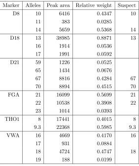
Table 3: Evett data showing mixture composition, peak areas and relative weights from a 10:1 mixture of two individuals, with suspect’s genotype specified.
Marker Alleles Peak area Relative weight Suspect
D8 10 6416 0.4347 10
11 383 0.0285
14 5659 0.5368 14
D18 13 38985 0.8871 13
16 1914 0.0536
17 1991 0.0592
D21 59 1226 0.0525
65 1434 0.0676
67 8816 0.4284 67
70 8894 0.4515 70
FGA 21 16099 0.5699 21
22 10538 0.3908 22
23 1014 0.0393
THO1 8 17441 0.4015 8
9.3 22368 0.5985 9.3
VWA 16 4669 0.4170 16
17 931 0.0884
18 4724 0.4747 18
19 188 0.0199
Table 4: Logarithm of the likelihood ratios in favour of H0 :u&s vs. H1 : 2u
for the Evett data.
Areas Alleles Assumed known mixture proportion
θ 0.1 0.2 0.3 0.4 0.5 0.6 0.7 0.8 0.9
[image:16.595.73.539.645.692.2]The absolute value of the likelihood ratios are slightly different from those given by [11], who report a logarithm of the likelihood ratio of 7.3. This discrepancy is most likely due to slight differences between our model and the model used by [11]. On the other hand, they report a likelihood ratio based on allele presence alone of 5800, whereas we find a ratio around 25000 using the gene frequencies reported in their paper, and insist the latter must be the correct value.
5
Separation of mixtures
Deconvolution of mixtures or separating a mixed DNA profile into its components has been studied by Perlin and Szabady [9], Wang et al. [10], and Bill et al. [8], among others. Here, we show how separation of mixtures can be solved by the same network model used for evidence calculations. A mixed DNA profile has been collected and the genotypes of one or more unknown individuals who have contributed to the mixture is desired, for example with the purpose of searching for a potential perpetrator among an existing database of DNA profiles.
For a two-person mixture, the easiest case to consider is clearly that of separation of a single unknown profile, i.e. when the genotype of one of the contributors to the mixture is known. The case when both contributors are unknown is more difficult. In the latter situation this is only possible to a reasonable accuracy when the contributions to the DNA mixture has taken place in quite different proportions.
We have chosen to show two alternative methods for predicting the genotype of the unknown contributor(s). In the first method we report the most probable genotype (or pair of genotypes) of the unknown contributor(s) for each marker separately. This result is obtained directly from the standard propagation method in the probabilistic expert system, known as sum-propagation. Note that this genotype is not necessarily the jointly most probable across markers. We therefore also report the joint probability of the genotypes chosen in this way. If this happens to be larger than 0.5, the most probable genotype has clearly been identified.
The second method calculates, by a method termed semimax-propagation, the most likely joint configuration of all unobserved discrete nodes, given the evidence available, and reports the genotypes of the unknown contributor(s) associated with this configuration. The semimax propagation first integrates over all unobserved continuous variables and then performs max-propagation as described in [12], Section 6.4.1, to identify the most probable configuration. Note again, that this may not be the most probable genotype across markers. There is no general efficient method for calculating the latter, but identifying the two configurations above and reporting their joint probabilities would be fully satisfactory for most purposes as they are most interesting when their joint probability is high.
tend to give identical results. It then also holds that the joint posterior probability of the genotypes of the unknown contributors is approximately equal to the product of those probabilities for each marker separately.
It would seem appropriate to report a list of probable genotypes for the unknown contributor(s), with their associated probabilities, but this would demand a slightly more sophisticated calculation and is beyond the scope of this particular paper.
5.1
Separating a single unknown profile
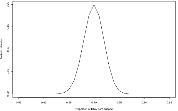
Our next example uses data from Perlin and Szabady [9], henceforth referred to as the
Perlin data, displayed in Table 5.
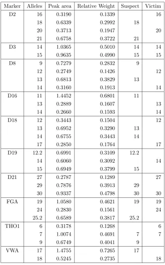
The two individuals contributing to the mixture are here namedsuspect andvictim and Table 6 displays the predicted genotype of the suspect, using information from the victim alone.
As in [9] the genotype of the unknown contributor is essentially determined exactly and the posterior distribution of the mixture proportion concentrates around the true value of 0.7, as displayed in Figure 4.
0.55 0.60 0.65 0.70 0.75 0.80 0.85
0.00
0.05
0.10
0.15
0.20
Proportion of DNA from suspect
[image:18.595.147.450.388.578.2]Posterior density
Figure 4: Posterior distribution of the mixture proportion for the Perlin data, using geno-typic information on the victim only.
Table 5: Perlin data showing mixture composition, peak areas, relative weights, suspect’s and victim’s genotypes from a 7:3 mixture of two individuals.
Marker Alleles Peak area Relative Weight Suspect Victim
D2 16 0.3190 0.1339 16
18 0.6339 0.2992 18
20 0.3713 0.1947 20
21 0.6758 0.3722 21
D3 14 1.0365 0.5010 14 14
15 0.9635 0.4990 15 15
D8 9 0.7279 0.2832 9
12 0.2749 0.1426 12
13 0.6813 0.3829 13
14 0.3160 0.1913 14
D16 11 1.4452 0.6801 11
13 0.2889 0.1607 13
14 0.2660 0.1593 14
D18 12 0.3443 0.1504 12
13 0.6952 0.3290 13
14 0.6755 0.3443 14
17 0.2850 0.1764 17
D19 12.2 0.6991 0.3109 12.2
14 0.6060 0.3092 14
15 0.6949 0.3799 15
D21 27 0.2787 0.1289 27
29 0.7876 0.3913 29
30 0.9337 0.4798 30 30
FGA 19 1.0580 0.4621 19 19
24 0.2830 0.1561 24
25.2 0.6589 0.3817 25.2
THO1 6 0.3178 0.1268 6
7 1.0074 0.4691 7 7
9 0.6749 0.4041 9
VWA 17 1.4755 0.7265 17
Table 6: Predicted genotype of suspect for thePerlin data, using genotype information for victim only. All markers are correctly identified by both sum and semi-max propagation.
Marker Genotype Probability
D2 18 21 1
D3 14 15 1
D8 9 13 1
D16 11 11 1
D18 13 14 1
D19 12.2 15 1
D21 29 30 1
FGA 19 25.2 1
THO1 7 9 1
[image:20.595.211.394.499.693.2]VWA 17 17 1
Table 7: Predicted genotype of suspect for Graham data, using genotype for victim only. All markers are correctly identified by both sum and semi-max propagation. The number in brackets is the product of individual marker probabilities.
Marker Genotype Probability D3 16 17 0.982624
D5 7 12 1
D7 10 10 0.984372
D8 13 16 1
D13 9 11 0.995181
D18 12 15 1
D21 30.2 31.2 1
FGA 23 25 1
VWA 16 18 1
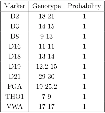
Table 8: Predicted genotype of contaminator for Evett data, using information from sus-pect. Identical results are obtained using sum and semi-max propagation. The number in brackets is the product of individual marker probabilities.
Marker Genotype Probability D8 11 14 0.834050
D18 16 17 1
D21 59 65 1
FGA 21 23 0.815391 THO1 9.3 9.3 0.826110
VWA 17 19 1
joint 0.567333 (0.561818)
The situation for theGrahamdata is similar to thePerlindata: all markers are correctly identified, with probabilities very close to 1 in all cases. Analysis of the Evett data yield probabilities between 0.8 and 1 on all markers. Evett et al. [11] does not contain the genotype of the second contributor so we do not know whether there are classification errors for this example. Figure 3 and Figure 5 display the posterior distribution of the mixture proportion for these two cases.
5.2
Separating two unknown profiles
We now turn to the problem of separating a mixture into two components, using peak area and repeat number information but no information regarding the two contributors to the mixture. Using only this information will lead to an identifiability problem in assigning genotype combinations to each person, because of the symmetry between the individuals p1 and p2 in the network of Figure 20 or in the equivalent object-oriented network Figure 18. To remove this problem it is sufficient to enter evidence that the pre-amplification proportion of DNA in the sample from individual p1 is at least one half of the total DNA in the sample. (The alternative, that individual p1 contributes at most half of the DNA to the mixture sample could as equally well be used to break the symmetry.) Using Hugin
this symmetry breaking may be achieved by entering likelihood evidence directly into the fraction node; in Maies direct entering of likelihood evidence is not possible, so instead
0.20 0.25 0.30 0.35 0.40 0.45 0.50
0.00
0.05
0.10
0.15
0.20
Proportion of DNA from suspect
[image:22.595.147.449.127.320.2]Posterior density
Figure 5: Posterior distribution of mixture proportion for Graham data using genotypic information from the victim only.
does imply is that the posterior distribution of the pre-amplification fraction will be zero for values greater than 0.5.
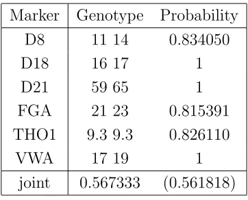
Our first example uses the Evett data, ignoring the information on the suspect. The posterior distribution of the mixture proportionθis displayed as the solid curve in Figure 6. The distribution is similar in shape to that in Figure 3, which uses the suspect genotype information. The broken curve in Figure 6 shows the posterior using the larger variance factor σ2 = 0.1. We note that this change of variance by an order of magnitude has a
notable effect on the posterior distribution of mixture proportion.
The predicted genotypes of the two contributors are shown in Table 9, with the suspect’s profile being predicted correctly for both choices of variance even though the probability of the chosen genotype is strongly reduced when the larger variance factor is used. Note that the probabilities in the left half of Table 9 are the same as those in Table 8 (to the accuracy given). This would not normally be expected, but for this example it turns out that in separating the profiles the genotype of person 1 is predicted with high certainty to be the same as the suspect. Hence adding in the suspect’s profile as was done for the calculations of Table 8 would have very little affect on the predictions made by the system for the genotype of the contaminator.
0.80 0.85 0.90 0.95 1.00
0.00
0.05
0.10
0.15
Proportion of DNA from the major contributor
[image:23.595.70.544.541.693.2]Posterior density
Figure 6: Posterior distribution of mixture proportion fromEvett data using no genotypic information: solid line σ2 = 0.01, broken line σ2 = 0.1.
Table 9: Predicted genotypes of both contributors for Evett data with σ2 = 0.01 and
σ2 = 0.1. Identical results are obtained using sum and semi-max propagation, with suspect
(p1) correct on every marker. The number in brackets is the product of individual marker probabilities.
σ2= 0.01 σ2 = 0.1
Marker Genotype p1 Genotype p2 Probability Genotype p1 Genotype p2 Probability
D8 10 14 11 14 0.834050 10 14 11 14 0.654367
D18 13 13 16 17 1 13 13 16 17 0.876868
D21 67 70 59 65 1 67 70 59 65 0.999405
FGA 21 22 21 23 0.815391 21 22 21 23 0.489847
THO1 8 9.3 9.3 9.3 0.826110 8 9.3 9.3 9.3 0.574267
VWA 16 18 17 19 1 16 18 17 19 0.999390
extent for the marker D19.
Increasing σ2 by a factor of 10 to σ2 = 0.1 yields the posterior distribution forθ shown
by the broken line Figure 7. In this case the effect of choosing an inflated variance factor is dramatic, also yielding reduced genotype probabilities and several classification errors as shown in Table 11. Note also that here there is a marked discrepancy between probability of the joint genotype and the product of the probabilities for each marker.
0.50 0.55 0.60 0.65 0.70 0.75 0.80
0.00
0.05
0.10
0.15
Proportion of DNA from the major contributor
Posterior density
Figure 7: Posterior distribution of mixture proportion fromPerlin data using no genotypic information: solid line σ2 = 0.01, broken line σ2 = 0.1.
Similar behaviour occurs in our third example that uses the Graham data. The pos-terior distribution of θ is shown as the solid curve in Figure 8, with a maximum for the major contributor around 0.65; the predicted profiles are shown in Table 12, with one clas-sification error. However note for this clasclas-sification error (in D7, using sum-propagation) the probability assigned to the genotype pair is around 0.66, with the correct classification (picked out by the semi-max method) having a probability of around 0.33. Note that the two chosen genotypes together account for essentially all of the probability mass.
Increasing the variance factor σ2 to 0.1 yields more classification errors but is also
Table 10: Predicted genotypes of both contributors for Perlin data with σ2 = 0.01. The number in brackets is the product of individual marker probabilities. For semi-max prop-agation all classifications are correct but for sum propprop-agation there is a classification error in marker VWA (italicized).
sum prop semi-max
Marker Genotype p1 Genotype p2 Probability Genotype p1 Genotype p2 Probability
D2 18 21 16 20 0.996545 18 21 16 20 0.996545
D3 14 15 14 15 0.974334 14 15 14 15 0.974334
D8 9 13 12 14 0.992179 9 13 12 14 0.992179
D16 11 11 13 14 0.994388 11 11 13 14 0.994388
D18 13 14 12 17 0.999520 13 14 12 17 0.999520
D19 12.2 15 14 14 0.796869 12.2 15 14 14 0.796869
D21 29 30 27 30 0.955125 29 30 27 30 0.955125
FGA 19 25.2 19 24 0.971191 19 25.2 19 24 0.971191
THO1 7 9 6 7 0.922004 7 9 6 7 0.922004
VWA 17 18 17 17 0.549705 17 17 18 18 0.393374
joint 0.353239 (0.358721) 0.261764 (0.256704)
0.50 0.55 0.60 0.65 0.70 0.75 0.80
0.00
0.05
0.10
0.15
Proportion of DNA from the major contributor.
Posterior density
[image:25.595.148.452.476.668.2]Table 11: Predicted genotypes of both contributors for Perlin data with σ2 = 0.1. The
number in brackets is the product of individual marker probabilities. There are classifica-tion errors in five markers (italicized).
sum prop semi-max
Marker Genotype p1 Genotype p2 Probability Genotype p1 Genotype p2 Probability
D2 18 21 16 20 0.285179 18 21 16 20 0.285179
D3 14 15 14 15 0.461512 14 15 15 15 0.229006
D8 9 13 12 14 0.279718 9 13 12 14 0.279718
D16 11 13 11 14 0.315883 11 11 13 14 0.270330
D18 13 14 12 17 0.291047 13 14 12 17 0.291047
D19 14 15 12.2 14 0.218410 12.2 15 14 14 0.170503
D21 29 30 27 30 0.357621 29 30 27 30 0.357621
FGA 19 25.2 19 24 0.324954 19 25.2 24 24 0.129379
THO1 7 9 6 7 0.322619 7 9 6 7 0.322619
VWA 17 18 17 17 0.364098 17 18 17 17 0.364098
joint 2.6978e-05 (1.0091e-05) 3.1643e-05 (1.332e-06)
Table 12: Prediction of two unknown genotypes for Graham data, with σ2 = 0.01. The
number in brackets is the product of individual marker probabilities. There is a classifica-tion error in marker D7 (italicized).
sum prop semi-max
Marker Genotype p1 Genotype p2 Probability Genotype p1 Genotype p2 Probability
D3 16 17 15 17 0.963136 16 17 15 17 0.963136
D5 7 12 13 13 0.994966 7 12 13 13 0.994966
D7 11 11 10 11 0.659653 10 10 11 11 0.326069
D8 13 16 12 12 0.835225 13 16 12 12 0.835225
D13 9 11 8 9 0.981719 9 11 8 9 0.981719
D18 12 15 13 13 0.931912 12 15 13 13 0.931912
D21 30.2 31.2 30 32.2 0.979851 30.2 31.2 30 32.2 0.979851
FGA 23 25 22 24 0.985227 23 25 22 24 0.985227
[image:26.595.73.542.512.710.2]Table 13: Prediction of two unknown genotypes for Graham data, using σ2 = 0.1. There
are now classification errors in six markers (italicized).
sum prop semi-max
Marker Genotype p1 Genotype p2 Probability Genotype p1 Genotype p2 Probability
D3 16 17 15 17 0.263132 16 17 15 17 0.263132
D5 7 13 12 13 0.311064 7 12 13 13 0.298917 D7 10 11 10 11 0.335654 10 10 11 11 0.133020 D8 12 13 12 16 0.310974 13 16 12 12 0.216863
D13 9 11 8 9 0.215735 11 11 8 9 0.133398
D18 12 13 13 15 0.300377 12 15 13 13 0.231450
D21 30.2 31.2 30 32.2 0.278259 30.2 31.2 30 32.2 0.278259
FGA 23 25 22 24 0.302807 23 25 22 24 0.302807
VWA 17 18 16 17 0.321188 16 18 17 17 0.262347
joint 1.7666e-05 (1.4983e-05) 6.9669e-06 (1.5486e-06)
5.3
An example using amelogenin
Our final example is taken from Appendix B of Clayton et al. [6] and illustrates the importance of theamelogenin marker in the analysis of DNA mixtures when the individual contributors are of opposite sex.
Peak area analysis of the amelogenin marker in DNA recovered from a condom used in a rape attack indicated an approximate 2:1 ratio for the amount of female to male DNA contributing to the mixture. Peak area information was available on six other markers, the information is shown in Table 14; we shall refer to this as the Clayton data.
In Table 15 we show the results of separating the mixture using peak area information only, without using information on the victim. All markers are correctly identified. Note in particular that the genotypes for the marker THO are identified correctly. Clayton et al. [6] were only able to do this after the victim’s profile was taken into account, because without this information the alternative genotype combination ({7,7},{5,5}) could also have explained the observed peak areas with an approximate 2:1 imbalance in the contrib-utors’ DNA. In our analysis we estimate that this alternative combination is around 258 times less likely than the correct designation.
Table 14: Clayton data showing mixture composition, peak areas and relative weights together with the DNA profiles of both victim and suspect. For the marker D21 the allele designation in brackets is as given in [6] using the Urquhart et al. [23] labelling convention
Marker Alleles Peak area Relative weight Suspect Victim
Amelogenin X 1277 0.8298 X XX
Y 262 0.1702 Y
D8 13 3234 0.6372 13
14 752 0.1596 14
15 894 0.2032 15
D18 14 1339 0.1462 14
15 1465 0.1714 15
16 2895 0.3612 16
18 2288 0.3212 18
D21 28 (61) 373 0.1719 28
30 (65) 590 0.2913 30
32.2 (70) 615 0.3259 32.2
36 (77) 356 0.2109 36
FGA 22 534 0.1547 22
23 2792 0.8453 23 23
THO 5 5735 0.2756 5
7 10769 0.7244 7 7
VWA 15 1247 0.1633 15
16 1193 0.1667 16
17 2279 0.3383 17
Table 15: Predicted genotypes of both contributors for Clayton data with σ2 = 0.01.
Identical results are obtained using sum and semi-max propagation, with victim (p1) and male suspect (p2) correct on every marker. The number in brackets is the product of individual marker probabilities.
σ2 = 0.01
Marker Genotype p1 Genotype p2 Probability
Amelogenin X X X Y 0.983115
D8 13 13 14 15 0.903013
D18 16 18 14 15 0.993166
D21 30 32.2 28 36 0.945235
FGA 23 23 22 23 0.989090
THO 5 7 7 7 0.845031
VWA 17 19 15 16 0.992738
joint 0.701988 (0.691517)
0.50 0.55 0.60 0.65 0.70 0.75 0.80
0.00
0.05
0.10
0.15
Proportion of DNA from the major contributor.
Posterior density
[image:29.595.147.449.452.652.2]6
Discussion
In the previous sections we have demonstrated how a probabilistic expert system can be used for analysing DNA mixtures using peak area information, yielding a coherent way of predicting genotypes of unknown contributors and assessing evidence for particular indi-viduals having contributed to the mixture. The advantages of a probabilistic model-based approach over numerical separation techniques such as Linear Mixture Analysis (LMA) [9] and Least Square Deconvolution (LSD) [10] are that there is a natural and directly interpretable quantification of all uncertainties associated with the analysis; in particular, the posterior distribution of the mixture proportion can be computed. Furthermore, the analysis is extendable to similar but different situations using the modularity and flexi-bility of the PES approach. This includes complications such as more than two potential contributors, multiple traces, indirect genotypic evidence, stutter, etc.
The examples considered have also demonstrated that there are issues which need further consideration. In particular it appears that the performance of the system is sensitive to large changes in the scaling factors we used to model the variation in the amplification and measurement processes. This is a serious problem which needs attention. Preliminary investigations seem to indicate that the variance factor depends critically on the totalamount of DNA available for analysis. As this necessarily is varying from case to case, a calibration study should be performed to take this properly into account. In any case we find it comforting that the system itself would warn against trusting an uncertain prediction, by yielding an associated low classification probability.
Methods for diagnostic checking and validation of the model should be developed based upon comparing observed weights to those predicted when genotypes are assumed correct. Such methods could also be useful for calibrating the variance parameters σ2 and ω2. To
indicate a possible way ahead we note that the network can itself be used for predicting peak weight given a hypothesized composition of the mixture and of the two contributors. Table 16 gives the predicted peak weights for thePerlin data based on the repeat numbers in the mixture composition, the true mixture composition, and on the suspect’s and victim’s genotype. The last two columns show the limits of the 95% predictive interval [µa −
1.96τ, µa+ 1.96τ] for the weight. For this purpose we use the variance structure (2) as
only the marginal distribution of the peak weights are involved so the correlations do not interfere. For a 95% predictive interval we might expect about one of the weights of the table to lie outside of its predicted interval, as about 21 of the 31 intervals are independent (the weights for each marker must add to one); all expected weights are within their intervals, indicating that the variance is not too small.
Table 16: Prediction of relative peak weight forPerlindata, using the mixture, the suspect’s and the victim’s DNA composition.
Marker Allele Relative Weight Predicted relative weight
µa−1.96τ µa+ 1.96τ
D2 16 0.1339 0.0565 0.2435
18 0.2992 0.2378 0.4622
20 0.1947 0.0565 0.2435
21 0.3722 0.2378 0.4622
D3 14 0.5010 0.3840 0.6160
15 0.4990 0.3840 0.6160
D8 9 0.2832 0.2378 0.4622
12 0.1426 0.0565 0.2435
13 0.3829 0.2378 0.4622
14 0.1913 0.0565 0.2435
D16 11 0.6801 0.5909 0.8091
13 0.1607 0.0565 0.2435
14 0.1593 0.0565 0.2435
D18 12 0.1504 0.0565 0.2435
13 0.3290 0.2378 0.4622
14 0.3443 0.2378 0.4622
17 0.1764 0.0565 0.2435
D19 12.2 0.3109 0.2378 0.4622
14 0.3092 0.1909 0.4091
15 0.3799 0.2378 0.4622
D21 27 0.1289 0.0565 0.2435
29 0.3913 0.2378 0.4622
30 0.4798 0.3840 0.6160
FGA 19 0.4621 0.3840 0.6160
24 0.1561 0.0565 0.2435
25.2 0.3817 0.2378 0.4622
THO1 6 0.1268 0.0565 0.2435
7 0.4691 0.3840 0.6160
9 0.4041 0.2378 0.4622
VWA 17 0.7265 0.5909 0.8091
Gaussian distributions can take negative values. Ideally the method should be generalized to deal with higher complexity such as the simultaneous analysis of several traces, an unknown but large number of contributors, etc., and we have not as yet made a proper investigation of the computational complexity issues associated.
We also will explore how to extend the model to handle Y-chromosome and mitochon-drial DNA haplotype data. Finally, we emphasize that for the moment we have not dealt with incorporating artifacts such as stutter, pull-up, allelic dropout, etc., but we hope to pursue this and other aspects in the future. It may be that in incorporating such artifacts our networks will become too complex for exact inference based on evidence propagation in Bayesian networks, and that a Monte-Carlo simulation approach may be required.
Acknowledgement
This research was supported by a Research Interchange Grant from the Leverhulme Trust. We are indebted to participants in the above grant and to Sue Pope and Niels Morling for constructive discussions. We thank Caryn Saunders for supplying the EPG image used in Figure 1. We also thank the associate editor and the referees for helpful comments.
References
[1] A. P. Dawid, J. Mortera, V. L. Pascali, and D. W. van Boxel. Probabilistic expert systems for forensic inference from genetic markers. Scand. J. Stat., 29 (2002) 577–595.
[2] L. A. Foreman, C. Champod, I. W. Evett, J.A. Lambert, and S. Pope. Interpreting DNA Evidence: A Review. Internat. Statist. Rev., 71 (2003) 473–495.
[3] J. Mortera, A. P. Dawid, and S. L. Lauritzen. Probabilistic expert systems for DNA mixture profiling. Theoret. Pop. Biol., 63 (2003) 191–205.
[4] I. W. Evett, C. Buffery, G. Wilcott, and D. Stoney. A guide to interpreting single locus profiles of DNA mixtures in forensic cases. J. Forensic Sci. Soc., 31 (1991) 41–47.
[5] B. S. Weir, C. M. Triggs, L. Starling, L. I. Stowell, K. A. J. Walsh, and J. S. Buckleton. Interpreting DNA mixtures. J. Forensic Sci., 42 (1997) 213–222.
[6] T. M. Clayton, J. P. Whitaker, R. Sparkes, and P. Gill. Analysis and interpretation of mixed forensic stains using DNA STR profiling. Forensic Sci. Int., 91 (1998) 55–70.
[8] M. Bill, P. Gill, J. Curran, T. Clayton, R. Pinchin, M. Healy, and J. Buckleton. PENDULUM — a guideline - based approach to the interpretation of STR mixtures. Forensic Sci. Int., 148 (2005) 181–189.
[9] M.W. Perlin and B. Szabady. Linear mixture analysis: a mathematical approach to resolving mixed DNA samples. J. Forensic Sci., 46 (2001) 1372–1378.
[10] T. Wang, N. Xue, and R. Wickenheiser. Least square deconvolution (LSD): A new way of resolving STR/DNA mixture samples. Presentation at the 13th International Symposium on Human Identification, October 7–10, 2002, Phoenix, AZ, 2002.
[11] I. Evett, P. Gill, and J. Lambert. Taking account of peak areas when interpreting mixed DNA profiles. J. Forensic Sci., 43 (1998) 62–69.
[12] R. G. Cowell, A. P. Dawid, S. L. Lauritzen, and D. J. Spiegelhalter. Probabilistic Networks and Expert Systems. Springer, New York, 1999.
[13] S. L. Lauritzen and F. Jensen. Stable local computation with conditional Gaussian distributions. Statistics and Computing, 11 (2001) 191–203.
[14] Y. Torres, I. Flores, V. Prieto, M. Lopez-Soto, M. J. Farfan, A. Carracedo, and P. Sanz. DNA mixtures in forensic casework: a 4-year retrospective study. Forensic Sci. Int., 134 (2003) 180–186.
[15] J. M. Butler, R. Schoske, P. M. Vallone, J. W. Redman, and M. C. Kline. Allele fre-quencies for 15 autosomal STR loci on U.S. Caucasian, African American and Hispanic populations. J. Forensic Sci., 48 (2003) 908–911. Available online at www.astm.org.
[16] T. M. Clayton and J. S. Buckleton. Mixtures. In S. J. Walsh J. S. Buckleton, C. M. Triggs, editor, Forensic DNA Evidence Interpretation, chapter 7, pages 217–274. CRC Press, 2004.
[17] R. G. Cowell, S. L. Lauritzen, and J. Mortera. Identification and separation of DNA mixtures using peak area information. Statistical Research Paper 25, Sir John Cass Business School, City University London, Nov 2004.
[18] P. Gill, R. Sparkes, and C. Kimpton. Development of guidelines to designate allele using an STR multiplex system. Forensic Sci. Int., 89 (1997) 185–197.
[19] D. Koller and A. Pfeffer. Object-oriented Bayesian networks. In Dan Geiger and Prakash P. Shenoy, editors, UAI ’97: Proceedings of the Thirteenth Conference on Uncertainty in Artificial Intelligence, August 1-3, 1997, Brown University, Providence, Rhode Island, USA, pages 302–313. Morgan Kaufmann, 1997.
August 1-3, 1997, Brown University, Providence, Rhode Island, USA, pages 302–313. Morgan Kaufmann, 1997.
[21] A. P. Dawid. An object-oriented Bayesian network for estimating muta-tion rates. In Christopher M. Bishop and Brendan J. Frey, editors, Pro-ceedings of the Ninth International Workshop on Artificial Intelligence and Statistics, Jan 3–6 2003, Key West, Florida, 2003. Available online at:
http://research.microsoft.com/conferences/AIStats2003.
[22] D. Cavallini and F. Corradi. OOBN for forensic identification through search-ing a DNA profiles’ database. In Robert G. Cowell and Zoubin Ghahra-mani, editors, Proceedings of the Tenth International Workshop on Artificial In-telligence and Statistics, Jan 6-8, 2005, Savannah Hotel, Barbados, pages 41– 48. Society for Artificial Intelligence and Statistics, 2005. Available online at:
http://www.gatsby.ucl.ac.uk/aistats.
[23] A. Urquhart, C. P. Kimpton, T. J. Downes, and P. Gill. Variation in short tandem repeat sequences – a survey of twelve microsatellite loci for use as forensic identification markers. Int. J. Leg. Med., 107 (1994) 13–20.
A
Likelihoods from peak area information
All Bayesian networks in the present paper have a common structure, as outlined below: The nodes corresponding to the observed relative peak weights R = (Ra, a= 1, . . . , A) are
all continuous. We are interested in the distribution P(D, M|R, E) where R denotes the peak weight,Eother types of evidence, e.g. evidence about genotypes of certain individuals,
M the nodes for the mean peak weights, andDthe remaining discrete nodes in the network. The mean peak weights are represented by discrete nodes with possible values µ = (µ1, . . . , µA). Using Bayes’ formula, and the fact that R is conditionally independent of
(D, E) given M, it holds that
P(D, M|R, E)∝P(R|M)P(D, M, E).
Thus, the information in the relative peak weights enter the calculations only through the peak weight likelihood
L(µ) =P(R|M =µ).
In the following we shall find a simple expression for this likelihood.
Consider now a vector X = (X1, . . . , XA) of independent and normally distributed
random variables with Xa∼ N(µa, τa2),i.e. with joint density
A (
where we have let µ= (µ1, . . . , µA) andT a diagonal matrix withτa2 as diagonal elements,
i.e. T = diag(τ2
1, . . . , τA2). We recall that
P
aµa = 1.
The distribution of the sum S = P
aXa is normal S ∼ N(1, τ2) with τ2 = Paτa2 and
the conditional distribution of X given S = 1 is itself multivariate normal with the same mean vector µand covariance matrix T∗, where
τ∗
aa =
τ2
a(τ2 −τa2)
τ2 , τ ∗
ab =
−τ2
aτb2
τ2 .
The density of the conditional distribution can now be calculated as
f∗(x
1, . . . , xA−1|µ, T∗)∝
f(x1, . . . , xA|µ, T)
fS(1|τ2)
∝τ f(x1, . . . , xA|µ, T), (4)
for xA= 1−PAa=1−1xa. If we consider the case
τa2 =σ2µa+ω2,
i.e. the variance structure in (3), we note that
τ2 =X
a
τa2 =σ2+Aω2
is constant in µ. Also the covariance matrixT∗ is
τ∗
aa =σ2µa(1−µa) +ω2+o(ω2), τab∗ =−σ2µaµb+o(ω2),
which, ignoring termso(ω2) which are an order of magnitude smaller thanω2, has precisely
the form (2) used in our model. If we ignore measurement error by setting ω2 = 0, the
entries in T∗ are exactly given by (2).
It follows that to an excellent approximation — exact for ω2 = 0 — we can calcu-late the correct peak weight likelihood based on T∗ by using the variance structure T with independence:
L(µ) = f∗(x
1, . . . , xA−1|µ, T∗)∝f(x1, . . . , xA|µ, T), which justifies the use of (3) in the calculations.
B
Description of the network classes in the
object-oriented network
B.1
The founder class
The classfounderof Figure 10 contains a single nodefounderwith the relevant repertory of alleles as its states, and an associated probability table describing their gene frequencies.
founder
Figure 10: Network founder for founder gene.
For illustration, we show marker FGA having observed alleles coded A to C and the aggregation of all unobserved alleles coded asx. The probability table is shown in Table 17.
Table 17: Gene frequencies for marker FGA as reported in Evett et al. (1998).
Allele A B C x
Frequency 0.187 0.165 0.139 0.509
B.2
The genotype class
The classgtin Figure 11 represents an individual’s genotype gt, formed by the unordered pair of paternal and maternal genes, {pg, mg}. (Input nodes pg and mg are copies of node
founder of classfounder.) The paternal and maternal genes, pg andmg, are chosen inde-pendently from the same population whose allele frequencies are assumed known. Output nodegt is the logical combination of input nodespg and mg.
B.3
The query class
The class whichgt of Figure 12 describes the selection between two genotypes.
If the Boolean node query? is true, then output node, outgt, will have identical genotype to ingt; otherwise it will be identical toothergt. This is written in the Hugin
expression language as: outgt := if(query? == true, ingt, othergt).4
4
mg pg
gt
Figure 11: Network gt for genotype.
outgt ingt
[image:37.595.208.389.185.321.2]query? othergt
B.4
The joint genotype
The network class jointgt of Figure 13 represents the combined genotype of two indi-viduals, p1 and p2. Node p1gt&p2gt is simply the logical combination of the two input genotypes in p1gt and p2gt.
p2gt p1gt
[image:38.595.212.394.207.316.2]p1gt&p2gt
Figure 13: Networkjointgt for genotype pairs.
B.5
The number of alleles
The class nallelesshown in Figure 14 counts the number, varying from 0 to 2, of a certain allelic type in a genotype. For allele A , nA := if(gt == AA, 2, if (or (gt == AB, gt == AC, gt == Ax), 1, 0)). Similarly, for B, C and x. This class models then(i)
a variables in
(1).
nA
gt
[image:38.595.266.345.505.605.2]B.6
The weight of an allele in the mixture
The class alleleinmix shown in Figure 15 shows whether a certain allelic type (repeat number) is in the mixture and computes its mean contribution to the peak area of the mixture.
n2A n1A
p2gt p1gt
meanA frac
[image:39.595.200.407.198.385.2]Ainmix?
Figure 15: Network alleleinmix for alleles in mixture.
Input nodesp1gtandp2gt, the genotypes of the two people, p1 and p2, contributing to the mixture, have identity links to the input nodegtin the two instances of classnalleles,
n1A and n2A. The Boolean node Ainmix? is true if at least one of the two contributors has allele A. Thus, Ainmix? := if(and (n1A nA == 0, n2A nA == 0), false, true), where
n1A nA and n2A nA refer to the output nodes of the two instances of class nalleles, n1A
and n2A. (Similar instances are built for the other alleles.) Repeat number information is entered and propagated from these nodes. For example, if the mixture contains allele A, nodeAinmix? is set totrue.
Input node frac represents the proportion of DNA contributed by p1, denoted by θ
in §2. To enable evidence propagation in the Bayesian network to be possible, we model this continuous variable by an approximating discrete variable. In our hand-built Hugin
B.7
The peak weight
The class peakweight shown in Figure 16 models the observable peak weight as in (1).
mean
weight
[image:40.595.260.342.174.396.2]weightobs
Figure 16: Network peakweight for peak weight.
The input node mean is identified, for example, with output node meanA of class al-leleinmix. The intermediate continuous nodeweightrepresents the unobserved true peak weight. This node has a conditional Gaussian distribution with mean given by the value of the discrete parent nodemeanand variance equal to 10∗0.01∗mean, representing variations in the amplification process, cf.§2. The observed peak weight is modelled by the continu-ous node weightobs to allow for additional measurement error of the true weight. When using peak area information the value of the relative peak weight is inserted as evidence in the node weightobs.
B.8
The target class
p1=s? p2=v?
[image:41.595.204.406.124.233.2]target
Figure 17: Network target.
B.9
The marker class
The classmarkerin Figure 18 is an upper level network containing several instances of the classes defined above. This class is made to represent information related to a particular marker. Here it is illustrated for a marker having three alleles represented in the mixture. Input nodesspg,smg,u1pg,u1mg,vpg,vmg,u2pgandu2mg are all copies of nodefounder
of class founder; u1 and u2 being two unspecified individuals. Input nodes p1=s? and
p2=v? are identified with the corresponding output nodes of classtarget. The nodessgt,
u1gt, vgt and u2gt are all instances of class gt. Evidence on the suspect’s and victim’s genotypes is entered in the network in the nodes sgt and vgt. Nodes p1gt and p2gt are instances ofwhichgtand whenp1=s? istrue (false),p1gtwill be identical tosgt(u1gt). A similar relationship holds between nodesp2=v?, p2gt,vgtandu2gt. The nodejointgt
is an instance of jointgt; Amean, Bmean, Cmean and xmean are instances of alleleinmix;
Aweight, Bweight,Cweight and xweight are instances of peakweight. Input node frac
is identified with the corresponding node in the master network described below.
B.10
The master network
Figure 19 gives the master network used for both identification and separation of DNA mixtures from two contributors. It refers to the data from [11] shown in Table 3.
jointgt
xweight Cweight
Bweight Aweight
xmean Cmean
Bmean Amean
p2gt p1gt
u2gt
vgt
sgt u1gt
frac
u2pg u2mg vpg vmg
u1pg u1mg spg smg
[image:42.595.99.504.277.532.2]p2=v? p1=s?
B.11
Amelogenin marker
To build a network for amelogenin one needs to make the following changes to the previous classes. No founder class is needed and the genotype class has a single output node gt
with states XX for female and XY for male, with equal prior probabilities. The query and jointgt classes only need trivial modifications to reduce their state spaces. The allele counting classnalleles, for a male contributor,gt== XY, (for a female contributor,gt== XX) has nX==1 (2) and nY== 1 (0). The class alleleinmix of §B.6, is modified so that
Xinmix? is set to true. All other network classes remain unchanged.
C
Description of the networks generated by Maies
The Bayesian network generated byMaies may be considered equivalent to an “unfolded”
version of the object-oriented networks described in Appendix B. An example of a network generated for a single marker with two alleles observed in the mixture is shown in Figure 20. The structure is similar to the network shown in Figure 18, and like the object-oriented network described earlier there are several distinct modules of repetition that can be seen in the figure: indeed it is this repetitive structure that makes it possible for Maies to
create the much larger Bayesian networks required to analyse mixtures on several markers. We now describe these various structures and how they interrelate.
C.1
Founding people
Maies currently assumes that DNA from two individuals are in the mixture. Thus it
sets up nodes for four founding individuals who are paired up, prefixed bys (for suspect),
v (for victim), and u1 and u2 representing two unspecified persons from the population. Corresponding to each of these individuals is a triple of nodes representing their genotype on the marker, and the individuals’ paternal and maternal genes. They are joined up as in Figure 11 and their function is the same. The probability tables associated with the maternal and paternal genes contain the allele frequencies of the observed alleles, whilst the conditional probability table associated with the genotype node is the logical combination of the maternal and paternal gene.
C.2
Actual contributors to the mixture
The genotypes on the marker of the two individuals p1 and p2 whose DNA is in the mixture are the nodes labelled p1gt and p2gt. Node p1gt has incoming arrows from nodes u1gt,
u2pg u2mg
vpg vmg
spg smg
u1pg u1mg
u1gt sgt vgt u2gt
p2 = v? p1 = s?
p2gt target
p1gt
p2 x p2 9
p2 8 jointgt
p1 x p1 9
p1 8
x inmix ? 9 inmix ?
8 inmix ?
x weightobs x weight 9 weight
8 weightobs 8 weight
9 weightobs sym
[image:45.595.123.480.248.532.2]p1 frac
The node labelled target represents the four possible combinations of values of the two nodesp1 = s? and p2 = v? as in Figure 17 and described in §B.8.
The network also has a node representing the joint genotypes of individuals p1 and p2, which is labelled jointgt, with incoming arrows fromp1gt and p2gt; the function of this part of the network is equivalent to the object shown in Figure 13.
C.3
Allele counting nodes
On the level below the genotype nodes for p1 and p2 is a set of nodes representing the number of alleles (taking the value of 0, 1 or 2) of a certain type in each individual. Thus, for example, the nodep1 8counts the number of alleles of repeat number 8 in the genotype of individual p1 for the given marker: this value only depends upon the genotype of the individual p1 and hence there is an arrow from p1gt to p1 8. These nodes model the n(i)
a
variables introduced in (1).
C.4
Repeat number nodes
On the level below the allele counting nodes are the repeat number nodes, labelled8 inmix?,
9 inmix? and x inmix?. These are (yes,no) binary valued nodes representing whether or not the particular alleles are present in the mixture: thus for example allele 8 is present in the mixture if either of the allele counting nodes p1 8 or p2 8 takes a non-zero value. For the nodex inmix? thexrefers to all of the alleles in the marker that are not observed. When using repeat number information as evidence the repeat number nodes present in the mixture will be given the value yes; all other nodes, including x inmix?, will be given the value no.
C.5
True and observed weight nodes
These nodes are represented by the rounded rectangle shapes. The nodes 8 weight,
9 weight and x weight represent the true relative peak weights r8, r9 and rx
respec-tively of the alleles 8, 9 and x in the amplified DNA sample; the nodes 8 weightobs,
9 weightobs and x weightobs represent the measured weights. The observed weight is given a conditional-Gaussian distribution with mean the true weight, and variance
ω2. Each true-weight node is given a conditional-Gaussian distribution with mean µ
a =
{θn(1)
a + (1−θ)n(2)a }/2, where the fractionθ of DNA from p1 in the mixture is modelled in
the network by a discrete distribution in the node labelled p1 frac. The variance is taken to be σ2µ
a, as specified in §2.
C.6
Networks with more than one marker
The network displayed in Figure 20 generated byMaies is for a single marker; for mixture