Reynolds number dependence of mean flow structure in square duct turbulence

City, University of London Institutional Repository

Citation:

Pinelli, A., Uhlmann, M., Sekimoto, A. & Kawahara, G. (2010). Reynolds number

dependence of mean flow structure in square duct turbulence. Journal of Fluid Mechanics,

644, pp. 107-122. doi: 10.1017/S0022112009992242

This is the accepted version of the paper.

This version of the publication may differ from the final published

version.

Permanent repository link:

http://openaccess.city.ac.uk/15264/

Link to published version:

http://dx.doi.org/10.1017/S0022112009992242

Copyright and reuse: City Research Online aims to make research

outputs of City, University of London available to a wider audience.

Copyright and Moral Rights remain with the author(s) and/or copyright

holders. URLs from City Research Online may be freely distributed and

linked to.

City Research Online:

http://openaccess.city.ac.uk/

publications@city.ac.uk

structure

in square duct turbulence

A L F R E D O P I N E L L I

, M A R K U S U H L M A N N

,

A T S U S H I S E K I M O T O

A N D

G E N T A K A W A H A R A

1

Modeling and Numerical Simulation Unit, CIEMAT, 28040 Madrid, Spain

2

Turbulent Flow Group, Institute for Hydromechanics, University of Karlsruhe, Germany

3_{Department of Mechanical Science, Osaka University, 560-8531 Osaka, Japan}

(Received 4 August 2009)

We have performed direct numerical simulations of turbulent flows in a square duct considering a range of Reynolds numbers spanning from a marginal state up to fully de-veloped turbulent states at low Reynolds numbers. The main motivation stems from the relatively poor knowledge about the basic physical mechanisms that are responsible for one of the most outstanding feature of this class of turbulent flows: Prandtl’s secondary motion of second kind. In particular, the focus is upon the role of flow structures in its generation and in its characterization when increasing the Reynolds number. We will present a two-fold scenario. On one hand, buffer layer structures determine the distri-bution of mean streamwise vorticity. On the other hand, the shape and the quantitative character of the mean secondary flow, defined through the mean cross stream function, are influenced by motions taking place at larger scales. It will be shown that high velocity streaks are preferentially located in the corner region (e.g.,lessthan 50 wall units apart from a side wall), flanked by low velocity ones. These locations are determined by the positioning of quasi streamwise vortices with a preferential sign of rotation in agreement with the above described velocity streaks’ positions. This preferential arrangement of the classical buffer layer structures determines the pattern of the mean streamwise vorticity which approaches the corners with increasing Reynolds number. On the other hand, the center of the mean secondary flow, defined as the position of the extrema of the mean cross stream function (computed using the mean streamwise vorticity), remains at a con-stant location departing from the mean streamwise vorticity field for larger Reynolds numbers, i.e. it scales in outer units. This paper also presents a detailed validation of the numerical technique including a comparison of the numerical results with data obtained from a companion experiment.

1. Introduction

Melling & Whitelaw 1976) as well as direct and large eddy simulations (Gavrilakis 1992; Madabushi & Vanka 1991) have provided useful reference data for the mean velocities and the Reynolds stress tensor. Those studies were mainly focused upon the budget of the averaged flow equations, while not providing much information on the underlying physical mechanisms responsible for the formation of secondary flow.Huser & Biringen (1993) attempted to relate the appearance of secondary flow to an interaction of ejection events between adjacent walls in the corner region. In a recent paper (Uhlmannet al.

2007), we have considered in detail the case of the marginal Reynolds number regime in this geometry. By marginal regime we mean the limiting behavior of the turbulent flow at Reynolds numbers on the verge of relaminarization (i.e., bulk Reynolds number in the order of 1100 corresponding to a friction Reynolds number of about 80). In this regime, strong evidence has been presented that the buffer layer coherent structures play a crucial role in the appearance of secondary flow of Prandtl’s second kind and in the deformation of the mean streamwise velocity profile. In particular, it has been shown that the deformation of the mean streamwise velocity profile is due to the presence of a persistent low velocity streak preferentially located over the center of the edges. Also it has been shown that there exists a matching between the preferential positions of quasi-streamwise vortices flanking the streak and the pattern of the mean secondary vorticity. Similar mean flow patterns have been observed in a recent study (Biauet al.

2008) that analyzed the time evolution of initial streamwise sub-optimal disturbances at a value of the Reynolds number close to relaminarization. When considering higher Reynolds numbers, other effects may appear. First of all, motions at different scales would play a role whereas in the low Reynolds number cases the cross-stream scale of coherent structures is comparable with the duct width. Also the length of the edge of the square cross section expressed in wall coordinates increases therefore allowing for the simultaneous presence of multiple pairs of high and low velocity streaks, meaning that in the flow region close to the center of each edge the flow would behave more and more like a turbulent plane Poiseuille flow without any preferential positioning of the buffer layer structures.

The main motivation of the present paper is to further pursue the idea that the sec-ondary flow is a footprint of the coherent motions embedded in the turbulent flow. Evidences of this conjecture will be given by means of numerical results obtained by direct numerical simulation performed at higher Reynolds numbers (i.e., higher than the marginal one) where several pairs of streaks and associated streamwise vortices can be accommodated simultaneously near each wall (i.e. at the same streamwise location, but separated in the spanwise coordinate). In particular, we propose a scenario in which the position of the center of the mean secondary vortices (the location of the extrema of the mean streamwise vorticity) is determined by the preferential positioning of quasi streamwise vortices associated with a high speed streak located close to each one of the corners. On the other hand, the change of the pattern of the mean secondary velocity streamlines at higher Reynolds numbers is induced by the presence of motions at larger scales. Before introducing and motivating our main conclusions, the numerical code is briefly illustrated together with comparisons with both previous numerical studies and experimental results.

2. Numerical Methodology

L x 1

−1

−1

H=2h z/h

Figure 1.Coordinates system and geometry of the duct

figure 1). The time evolution of the velocity vector u= (u, v, w) (u alongx, v along y

and walong the z direction) and of the pressure pare governed by the incompressible Navier-Stokes equations

∂tu+∇p=−(u· ∇)u+ 1

Reb

∇2_{u, (2.1}

a)

∇ ·u= 0, (2.1b)

written in non dimensional form with density fixed to unity and the Reynolds number,

Reb=Ubh/ν, formed with the bulk velocityUb, the duct semi heighthand the kinematic viscosity ν. For convenience, we also introduce the definition of the friction Reynolds number asReτ =uτh/ν withuτ=

p

τw/ρthe friction velocity,τwbeing the wall shear stress averaged in time and on the four limiting walls andρthe constant density. The velocity vector is subject to the no-slip and impermeable conditions at the walls, while periodic conditions are specified at the cross stream boundary faces.

We employ an incremental-pressure projection method for splitting the system (2.1) into two fractional steps. Using a semi-implicit scheme for the viscous terms and a three-step low-storage Runge-Kutta method with an explicit treatment for the non-linear terms, the semi-discrete system can be written as follows:

u∗_−uk−1

∆t =−γk[(u· ∇)u]

k−1

−ζk[(u· ∇)u]k−2

−2αk∇pk−1+

αk

Reb

∇2 _u∗+uk−1

(2.2a)

∇2_φk ₌ ∇ ·u∗

2αk∆t (2.2b)

uk=u∗_{−2αk∆t∇φ}k _(2.2

c)

pk=pk−1_+φk₋αk∆t

Reb

∇2_φk _(2.2

d)

velocity. The auxiliary variable φ, sometimes called “pseudo-pressure”, is the projector onto the divergence free space.The boundary condition for φ in (2.2b) is ∂φ_∂nk = 0 for all the Runge-Kutta sub steps, being n the normal direction to the wall. The follow-ing set of coefficients (Verzicco & Orlandi 1996) leads to overall second-order temporal accuracy for both velocity and pressure in the interior of the computational domain:

αk =154, 1 15,

1

6 , γk=

8 15,

5 12,

3

4 andζk =

0,−17

60,− 5

12 . On the walls, due to the use

of the fractional step scheme, the no-slip condition is verified up to an error ofO(∆t2_ν).

In the worst case (corresponding to the lowest considered Reynolds number), the slip errorwas kept below 10−4_U

bby adjusting the time step ∆taccordingly. Flow variables are expanded in space by means of truncated Fourier series in the streamwise direction, while Chebyshev polynomials are used in the two cross-stream directions. The collocation points in the cross-stream directions are the standard Gauss-Chebyshev-Lobatto points, while a grid of equispaced nodes is defined in the streamwise direction. The non-linear terms in (2.2a) are evaluated in physical space whereas the linear explicit terms are eval-uated in spectral space. The fields are transformed back and forth by means of FFT and FCT. Dealiasing according to the 2/3-rule is performed in the Fourier direction only. The solution of the Helmholtz equations for the predicted velocity components (2.2a) and the Poisson equation for pseudo-pressure (2.2b) are carried out in physical space for each streamwise wave number by means of a fast diagonalization technique (Haldenwanget al.

1984). All the simulated cases have been computed imposing a constant flow rate. To this end, the Fourier zero mode of the stream-wise velocity component is adjusted after each Runge-Kutta sub-step in the predictor phase. In particular, an unknown constant pressure gradientA∗_{is introduced in (2.2a) when considering the zero Fourier component}

of the predicted streamwise velocity ˆu∗

0(y, z) :

∇2 ₋ Re αk∆t

ˆ

u∗

0(y, z) = ˆF0 u

k−1_{, u}k−2_{, p}k−1

+A∗_{, (2.3)}

where ˆF0 contains all the contributions from explicit terms in equation (2.2a) to the zero mode . The solution of problem (2.3) is decomposed as a linear combination of two contributions. The first one ˆu1

0 is the solution of (2.3) withA∗= 0, while the second ˆu20

is obtained solving the problem

∇2 − Re αk∆t

ˆ

u20(y, z) = 1. (2.4)

Both solutions are obtained using Dirichlet homogeneous conditions on the square bound-ary. The final solution is assembled as

ˆ

u∗

0(y, z) = ˆu 1 0+A∗uˆ

2

0 (2.5)

withA∗ _{obtained from the requirement:}

Qf =

Z

Ω

ˆ

u10 dydz+A∗

Z

Ω

ˆ

u20dydz (2.6)

withQf = 4h2Ub the desired flow rate through section Ω.

3. Validation

y/h

0 1 2

−1 −0.8 −0.6 −0.4 −0.2

hui/Ub

y/h

−0.02−1 0 0.02

−0.8 −0.6 −0.4 −0.2

hwi/Ub

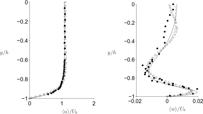
Figure 2.Mean velocity components atz/h=−0.7: streamwise component (left), cross stream component (right). Present DNS results (——Reb= 3500 – – – –Reb= 2205) compared to refer-ence DNS data (◦) and experimental data (•).

2205, as previously simulated by Gavrilakis (1992) and another case at a slightly higher Reynolds number (i.e., Reb = 3535) for which a set of experimental data (Kawahara

et al.2000) is available. Our simulations were both performed with a streamwise period ofLx/h= 4π, which can be considered sufficiently long in order to allow for an adequate decay of the two-point velocity correlations (Gavrilakis 1992, figure 3). For the lower Reynolds number case, we used 128 Fourier modes, corresponding to a streamwise grid spacing of ∆x+ _{= 14.7 (here and in the following, the superscript+stands for wall units:} l+_=l/δ

v withδv =ν/uτ the viscous length scale); 97 Chebyshev modes are employed in each cross-stream direction, leading to a spacing of 0.08≤∆y+_,∆z+ _{≤4.9. The time}

step was fixed at ∆t Ub/h= 1.93×10−2, approximately corresponding to aCF L= 0.22. Statistics were accumulated over an interval oftstatUb/h= 8000. It is worth mentioning that the time accumulated to compute statistical quantities is significantly larger than the one presented in the reference work (Gavrilakis 1992).In order to confirm that the actual streamwise discretization was fine enough to capture the behavior of typical buffer layer structures, higher resolution computations have been undertaken at Reb = 2205 using

192 Fourier modes in the streamwise direction (∆x+ _{< 10). No substantial difference} (less than 4%) has been found in the second order statistics of the velocity field. For the higher Reynolds number case, 192 Fourier modes were employed in the streamwise direction leading to the same wall coordinates spacing as in the previous case. In the cross stream plane, 129 nodes were used in both wall normal directions obtaining a grid spacing of 0.07≤∆y+_,∆z+_{≤5.2. The temporal resolution was ∆t U}

b/h= 0.5×10−3. Statistics, for the second case, were accumulated over a period oftstatUb/h= 5800. Details about the reference cases can be found in Gavrilakis (1992) and in Kawahara et al. (2000). In what follows we give a brief summary of the latter since the original work has never been published in English. The set of data was collected from experiments conducted in fully-developed turbulent flow in a straight water-duct (kinematic viscosityν = 0.94×

10−2_cm2_{/s). The duct has a square cross-section of an internal width 2h= 100mm and is}

y/h

a)

0 0.1 0.2

−1 −0.8 −0.6 −0.4 −0.2 0

hu′_u′_i1/2 /Ub

y/h

b)

0 0.1 0.2

−1 −0.8 −0.6 −0.4 −0.2 0

hu′_u′_i1/2 /Ub

y/h

c)

0 0.05 0.1

−1 −0.8 −0.6 −0.4 −0.2 0

hw′_w′_i1/2 /Ub

y/h

d)

0 0.05 0.1

−1 −0.8 −0.6 −0.4 −0.2 0

y/h

hw′_w′_i1/2 /Ub.

Figure 3. Profiles of the rms of the streamwise and cross stream velocity components at two different positions along one edge. Streamwise component,hu′_u′_i1/2_/U

b, atz/h=−0.3 (a) and atz/h=−0.7 (b). Cross stream component,hw′_w′_i1/2

/Ub, atz/h=−0.3 (c) and atz/h=−0.7 (d). Lines and symbols same as in figure 2

|ν∂hui/∂z| τw

−200 −100 0 100 200

0 0.5 1

y+

Figure 4.Mean local wall stress, normalized by the average over the whole wall, as a function of the distance along the wall in wall units. Symbols indicate the value of the bulk Reynolds number:▽, Re_b = 1077; ◦, Re_b = 1400; ₂,Re_b = 1753; △, Re_b = 2205; ⋄,Re_b = 2600; ∗,

Reb= 3500

directions respectively. At each measuring position, the data rate of Doppler signals ranged from 100Hz to 200Hz, and the total number of the signals was 105_−1.2×105_.

Next we present a comparison of the aforementioned reference data (numerical and experimental) against results obtained with our DNS. All the comparisons will be pro-vided in external units because of the experimental uncertainties in determining the skin friction velocity in the experiments. First, we compare and characterize the mean flow. Figure 2 (left) shows a nearly perfect collapse of our mean streamwise velocity profile (here and throughout the rest of the paper, the operatorh istands for time and stream-wise average) as compared to reference data at sectionz/h=−0.7. In the same figure, the profiles of the mean cross-stream velocity component are provided (right) at the same section. A certain level of disagreement with the experimental data is clearly visible far from the wall. Nonetheless, it should be noted that in the core regionhwi is orders of magnitude smaller than Ub. Therefore, even small deformation of the turbulence field by an uncertainty problem in the experimental apparatus could significantly affect the results.

Next, we compare the profile of the normal Reynolds stresses. In figures 3(a) and 3(b) profiles of thermsof streamwise velocity fluctuations (i.e.,u′ _{=u− hui) from our}

DNS are compared with the reference data at two different positions along the edge. A similar set of profiles, at the same locations, for the rms of the transversal velocity component (w′ _{=w− hwi) is given in figures 3(c) and 3(d) . Our DNS results for the}

normal Reynolds stresses are in excellent agreement with the experimental data. The comparison with the data of Gavrilakis (1992) again yields a very close match, except for the profile in figure 3(b) (i.e. forhu′_u′_i1/2_/U

4. Reynolds Number Dependence

Despite extensive study of the turbulent flow in a square duct using a variety of numerical techniques there remain significant questions about the scaling properties of the mean secondary flow and the associated distortion of the mean streamwise velocity profile. In what follows we will address the scaling of characteristic positions related to cross stream and streamwise mean motion within a range of marginal to low Reynolds numbers (Reb ≤ 3500). In this framework we will propose a physical explanation, in terms of coherent structure dynamics, of the pattern and scaling of the mean secondary motion.

All the simulations have been carried out in a careful manner with a time step such that CF L≤0.25 while keeping the slip error below 0.5×10−4 _U

b and by choosing the number of collocation nodes to guarantee a grid spacing verifying ∆x+_{≤15, and 0.05≤}

∆y+_{≤5 (same spacing criterion for ∆z}+_{). Statistical quantities were accumulated over}

time intervalststatUb/h≥7000. Also, all the computations have been carried out using comparable domain sizes: [−1,1]×[−1,1]×Lx/h, withLx= 10.97hto 12.57h.

4.1. Mean streamwise structure

Firstly, in order to characterize the shape of the mean streamwise profile, we present in figure 4 the mean local wall stress along one edge in wall coordinates. The skin friction coefficients, obtained averaging in time and along the streamwise direction, are in good agreement with the empirical formula: f−1_{2 = 2 log}

10(2.25Rebf 1

2)−0.8, f being the skin friction factor defined byf = 8u2

τ/Ub2(Jones 1976). At this level, it is important to mention that the above given empirical formula estimates that the length of the edge of the square in wall units spans the range 2 h+ _{∈[160,450] for the considered interval of}

Reynolds numbers (i.e.,Reb∈[1077,3500]). From the dimension of the square, expressed in wall units, one may anticipate an upper bound for the number of wall velocity streaks statistically facing each one of the four walls since the average distance between streaks of different velocity sign is of the order of 50+ _{(Kimet al. 1987). Therefore, for the lowest}

Reynolds number, one would expect an arrangement of a maximum of three velocity streaks, while for the highest an arrangement of a maximum of nine velocity streaks can be anticipated. Indeed, this argument is confirmed by figure 4. At the lowest values of the Reynolds number the profiles present two maxima and one minimum, indicating that a low velocity streak, flanked by two high velocity ones, is located preferentially at the center of the edge. At Reb = 2205 andReb = 2600, the situation changes since now the edge, measured in wall units (2h+_{≃300 and≃350, respectively), can host up}

d+

w

1000 1500 2000 2500 3000 3500

25 50 75 100

Reb

Figure 5.Distance to the cornerd+

w, in wall units, of the location along the edge of maximum and minimum ofτw closest to the corner as a function of Reb.◦is the position of maximum shear, the crosses represent the position of the location of minimum shear. Different crosses are used to highlight the discrete behavior of low velocity streak positioning. Dashed line is duct half width in wall unitsh+

as a function ofReb.

The location of maximum shear has a clear trend to level off with increasingRebat a value of about 50+ _{units. On the other hand, at approximately Re}

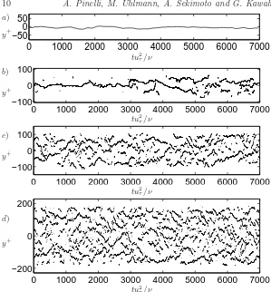
b = 2000 (corresponding to Reτ ≃ 120), the position of the minimum has a sharp change indicating that the wall, above this value, is hosting an average of 5 streaks. At higher Reynolds numbers, other jumps will probably appear consistently with the appearance of more velocity streaks on average along the edge. As further evidence of preferential streak locations as a function of Reynolds number, in figure 6 the time evolution of the location of low speed streaks along one edge is given in viscous coordinates at different bulk Reynolds numbers. These locations are instantaneously identified as the position of the minimum values of streamwise averaged wall shear stress. It can be seen that at the lowest Reynolds number a single low speed streak smoothly meanders about the center of the edge. When increasing the Reynolds number more than one simultaneous streak is detected. At the highest Reynolds number the path followed by the low speed streaks becomes less and less predictable without displaying any favorite positioning. This behavior is consistent with the observed flattening of the local mean skin friction of figure 4. Also, it should be noted that regions close to the corners (i.e.,y+_{≃ ±200) are seldom visited by low speed}

a)

y+

0 1000 2000 3000 4000 5000 6000 7000 −500

50

tu2

τ/ν

b)

y+

0 1000 2000 3000 4000 5000 6000 7000 −100

0 100

tu2

τ/ν

c)

y+

0 1000 2000 3000 4000 5000 6000 7000 −100

0 100

tu2

τ/ν

d)

y+

0 1000 2000 3000 4000 5000 6000 7000 −200

0 200

tu2

τ/ν

Figure 6.Time evolution of position of minimum of the streamwise averaged wall shear stress atz/h= 1:a)Reb= 1100,b)Reb= 1500,c)Reb=2205andd)Reb= 3500.

(cf. figure 5).In figure 8, the same analysis as in figure 7 is given for the high velocity streaks. At the lowest value of Reb the most probable scenario are two high velocity streaks flanking a low velocity one preferentially located at the edge midpoint. As for the case of low velocity streaks, when increasing Reynold number the probability of finding a high velocity streak along the edge becomes more and more uniform. The only locations that display a higher probability of hosting high speed streaks are the corner regions as opposed to the preferential absence of low velocity ones.

4.2. Mean cross flow structure

When focusing upon the mean value of the cross-stream velocity components, the well known pattern of mean secondary flow in the cross-plane of the square duct consisting of eight vortices, one counter-rotating pair being located above each of the four wall planes is observed. Their sense of rotation is such that the secondary flow on the diagonals is directed towards the corners (Gavrilakis 1992). Figure 9 displays isolines of the mean cross streamfunction hψi(y, z) computed from ∇2_{hψi(y, z) = −hω}

a)

−10 −0.5 0 0.5 1

0.5 1 1.5 2 2.5

y/h

b)

0 50 100 150 200 250

0 0.01 0.02 0.03 0.04 0.05 0.06

h+_+y+

Figure 7.Probability density function of low speed streak positions computed considering the instantaneous location of the minimum value of wall skin friction:a) in outer units andb) in inner units (the origin has been translated to the corner). Lines correspond to:——,Reb= 1100;

—•—,Reb= 1500;--·--·--,Reb= 2200;- - - -,Reb= 3500.

a)

−10 −0.5 0 0.5 1

0.5 1 1.5 2 2.5

y/h

b)

0 50 100 150 200 250

0 0.01 0.02 0.03 0.04 0.05 0.06 0.07 0.08

h+_+y+

Figure 8.Probability density function of high speed streak positions computed considering the instantaneous location of themaximumvalue of wall skin friction:a) in outer units andb)in inner units (the origin has been translated to the corner). Lines and symbols as in figure 7.

a smooth secondary flow as shown in Uhlmannet al.(2007). At higher Reynolds number values, vortical structures on a wider scale range appear. A lower bound for the latter are the quasi streamwise vortices associated with near-wall velocity streaks (dissipation scale). An upper bound is determined by the geometrical constraints (largest scales). In figure 10, contours ofhωxi(y, z) are given at the same three Reynolds numbers considered in figure 9. AtReb = 1077, the pattern of mean streamwise vorticity resembles the one of the mean streamfunction, except for the layer of mirrored wall vorticity. At higherReb values, the shapes of mean streamwise vorticity and streamfunction progressively depart from each other. In particular, the vortex centers and the stagnation points display a completely different behavior.

A more quantitative analysis of the dependence of the extrema of hωxi(y, z) and

y h

(a)

−1 −0.75 −0.5 −0.25 0 −1 −0.75 −0.5 −0.25 0 z/h y h

(b)

−1 −0.75 −0.5 −0.25 0 −1 −0.75 −0.5 −0.25 0 z/h y h

(c)

−1 −0.75 −0.5 −0.25 0 −1 −0.75 −0.5 −0.25 0 z/h

Figure 9.Streamlineshψi(y, z) of secondary mean flow computed usinghviandhwiaveraged over all quadrants (with increment [maxhψi−minhψi]/30). Dashed lines correspond to clockwise rotation, continuous lines to counterclockwise motion. (a)Reb= 1077; (b)Reb= 2205 and (c)

Reb= 3500. Only [−1,0]×[−1,0] quadrant shown.

y h

(a)

−1 −0.75 −0.5 −0.25 0 −1 −0.75 −0.5 −0.25 0 z/h y h

(b)

−1 −0.75 −0.5 −0.25 0 −1 −0.75 −0.5 −0.25 0 z/h y h

(c)

−1 −0.75 −0.5 −0.25 0 −1 −0.75 −0.5 −0.25 0 z/h

Figure 10.Iso-contours ofhωxi(y, z) of secondary mean flow averaged over all quadrants (with increment [maxhωxi−minhωxi]/30). Dashed lines correspond to negative values, continuous lines to positive ones. (a) Reb = 1077; (b) Reb = 2205 and (c) Reb = 3500. Only [−1,0]×[−1,0] quadrant shown.

of allowed streaks along the edge, as previously discussed, reflects clearly in the jump of the tangential distance (i.e. the distance to z/h = −1) of the minimum of hωxi at

Reb≃2000 (Reτ ≃150) as reflected in figure 11(a, b). This observation provides further evidence that the pattern of the mean streamwise vorticity is associated with the near wall coherent structures. Indeed, the position of the minimum of the mean streamwise vorticity has a clear trend to scale with viscous units, indicating a dependence on the wall structures. Moreover, the distance to the wall at z/h = −1 expressed in viscous units remains relatively constant and approximately corresponds to the position of the maximum of hω′

x ωx′i in a plane channel flow (Jim´enez & Moin 1991) that is located between 20+_{and 30}+_.

pat-s/h

1000 1500 2000 2500 3000 3500 4000 0

0.2 0.4 0.6

Reb

s+

50 100 150 200 250

0 25 50 75

Reτ

Figure 11.Positions of extrema ofhωxi: (a) external coordinates vsReband (b) wall coordinates vsReτ. Symbols:◦distance toz/h=−1;×distance toy/h=−1 (see dashed lines in figure 10)

(a)

s/h

1000 1500 2000 2500 3000 3500 4000 0

0.2 0.4 0.6 0.8 1

Reb

(b)

s+

50 100 150 200 250

0 25 50 75 100 125

Reτ

Figure 12. Positions of extrema of hψi(y, z): (a) external coordinates vs Reb and (b) wall coordinates vsReτ. Symbols:◦distance toz/h=−1;×distance to y/h=−1 (see solid lines

in figure 9)

terns that scale with the dimension of the latter (i.e., occupying the entire cross section) independently of the value ofReb.

pattern accumulated over the same interval (cf. figure 10b). This observation confirms that the mean streamwise vorticity pattern is a statistical portrait of the most probable locations of the quasi-streamwise vortices that are preferentially located in the corner regions. Furthermore, figure 13(c) presents a distribution of the p.d.f. in the close-to-the-wall regions consistent with the fact that, at this Reynolds number (i.e.,Reb= 2200), the most probable configuration on each edge is of two stronger high velocity streaks close to the corners and a milder one at the edge center(see figure 8). Indeed, the preferential location of the quasi-streamwise vortices (two counter rotating cores for each octant) induces a preferential positioning of fast velocity streaks in the same regions.

5. Conclusions

We have presented a numerical technique to simulate turbulent flows in infinitely long square ducts at constant flow rate. The numerical method has been validated against data from reference DNS and laboratory experiments.

Our analysis of the DNS results has focused upon the dynamical mechanisms that lead to the behavior of mean velocity values when increasing the Reynolds number: deformation of the mean streamwise velocity and the shape of mean secondary flow. It has been found that the mean streamwise velocity component depends upon the number of statistically allowed velocity streaks in the square. When increasing the Reynolds number the variation of wall shear along the spanwise coordinate smoothes out gradually except in the corner region where low velocity streaks are inhibited. In order to understand the scaling of the mean cross stream velocity components, we have considered both the behavior of the mean streamwise vorticity and of the mean cross stream function. The two quantities are shown to collapse at the lowest Reynolds number while progressively departing from each other when increasing the Reynolds number value. Evidence has been given that mean streamwise vorticity strongly depends upon statistically preferred location of the quasi-streamwise vortices associated with the pair of fast/slow streaks closest to the corner. Therefore a viscous scaling can be stated for such a mean quantity. On the other hand it has been found that the positions of the stagnation points of the mean cross flow streamfunction do not scale in viscous units but rather in external ones. The difference between the behavior of mean streamwise vorticity and mean stream-function in the crossflow plane stems from the fact that the latter is obtained as the solution of a Poisson equation (∇2_hψi=−hω

xi) with the former as r.h.s. Therefore, the

streamfunction exhibits non-local behavior (i.e. vorticity at any location influences the streamfunction everywhere), much alike the dependence between the pressure field and the divergence of the convective terms. As a consequence, there is no obvious reason why both quantities should scale equally. The precise implications of the relation between mean vorticity and streamfunction in duct flow, however, is beyond the scope of the present paper.

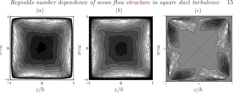
Within the considered range of Reynolds numbers, evidence has been given that the mean properties of the flow field depend upon the preferred positioning of buffer layer coherent structures. In particular, below Reb ≃ 2000 all the flow scales collapse, thus

making all the mean quantities a direct footprint of the actual most probable location of those structures: mean streamwise vorticity, mean cross stream function and the loci of the extrema of wall shear stress. At bulk Reynolds numbers higher than 2200, the influence of the coherent structures just reflects in the shape of the mean streamwise vorticity field and in the location of the local maximum of wall stress closest to the corner. The range ofRebaround 2100 is atransitionalregime in which the region facing

y h

−1 0 1

−1 0

z/h

y h

−1 0 1

−1 0

z/h

y h

−1 0 1

−1 0

z/h

Figure 13.Statistical data for the case with Reb= 2205 and Lx/h= 4π, accumulated from 1000 flow fields over a time interval of 1000h/Ub. (a) gray levels indicate .1(.1).9 times the maximum probability of occurrence of vortex centers withnegativestreamwise vorticity (white maximum, black minimum); (b) the probability for vortices withpositivestreamwise vorticity; (c) the difference of the probabilities of the location of positive (b) and negative vortex centers (a) averaged on the four quadrants (replicated on each quadrant for convenience).

In this range of Reynolds numbers the shape of the mean streamwise vorticity field, the local maximum of the wall shear near the corner, the local maximum of the wall shear on the wall bisector and the local minimum of the wall shear near the corner can be related to the distribution of the coherent structures.

To further investigate the eventual role of other, larger scales upon the mean flow structure higher Reynolds number simulations will be undertaken in the future.

The collaboration between the groups was supported by the Center of Excellence for Research and Education on Complex Functional Mechanical Systems (COE program of the Ministry of Education, Culture, Sport, Science, and Technology of Japan). M.U. was supported by the Spanish Ministry of Education and Science under contract DPI-2002-040550-C07-04. G.K. was partially supported by a Grant-in-Aid for Scientific Research (B) from the Japanese Society for the Promotion of Science.

REFERENCES

Biau, D., Soueid, H. & Bottaro, A.2008 Transition to turbulence in duct flow. J. Fluid Mech.596_{, 133–142.}

Brown, D.L., Cortez, R. & Minion, M.L.2001 Accurate projection methods for the incom-pressible Navier-Stokes equations.J. Comput. Phys.168_{, 464–499}

Brundrett, E. & Baines, W.1964 The production and diffusion of vorticity in duct flow.J. Fluid Mech.19_{, 375–394.}

Gavrilakis, S.1992 Numerical simulation of low-Reynolds-number turbulent flow through a straight square duct.J. Fluid Mech.244_{, 101–129.}

Gessner, F.1973 The origin of secondary flow in turbulent flow along a corner.J. Fluid Mech. 58_{, 1–25.}

Haldenwang, P., Labrosse, G., Abboudi, S. & Deville, M.1984 Chebyshev 3-d spectral and 2-d pseudo-spectral solvers for the Helmholtz equation.J. Comput. Phys.55_{, 115–128.}

Huser, A. & Biringen, S.1993 Direct numerical simulation of turbulent flow in a square duct.

J. Fluid Mech.257_{, 65–95.}

Jim´enez, J. & Moin, P.1991 The minimal flow unit in near-wall turbulence.J. Fluid Mech. 225_{, 213–240.}

Jones, O.1976 An improvement in the calculation of turbulent friction in rectangular ducts.

Kawahara, G., Ayukawa, K., Ochi, J. Ono, F. & Kamada, E.2000 Wall shear stress and Reynolds stresses in a low Reynolds number turbulent square duct flowTrans. JSME B 66_{(641), 95–102,(in Japanese).}

Kida, S. & Miura, H.1998 Swirl condition in low-pressure vortices.J. Phys. Soc. Japan67_(7),

2166–2169.

Kim, J., Moin, P. & Moser, R.D. 1987 Turbulence statistics in fully developed channel flow at low Reynolds number.J. Fluid Mech.177_{, 133–166.}

Madabhushi, R.K. & Vanka, S. P.1991 Large eddy simulation of turbulence-driven secondary flow in a square duct.Phys. of Fluids A3_{(11), 2734–2745.}

Melling, A. & Whitelaw, J.1976 Turbulent flow in a rectangular duct.J. Fluid Mech.78_,

289–315.

Nikuradse, J. 1926 Untersuchungen ¨uber die Geschwindigkeitsverteilung in turbulenten Str¨omungen. PhD Thesis, G¨ottingen.VDI Forsch.281_.

Prandtl, L. 1926 ¨Uber die ausgebildete turbulenz. Verh. 2nd Intl Kong. Fur Tech. Mech., Zurich[English transl.NACA Tech. Memo.435]

Uhlmann, M., Pinelli, A., Kawahara,. G. & Sekimoto, A.2007 Marginally turbulent flow in a square duct.J. Fluid Mech.588_{, 153–162.}