City, University of London Institutional Repository
Citation
:
Gerrard, R. J. G. and Tsanakas, A. (2010). Failure Probability Under Parameter Uncertainty. Risk Analysis, 31(5), pp. 727-744. doi: 10.1111/j.1539-6924.2010.01549.xThis is the accepted version of the paper.
This version of the publication may differ from the final published
version.
Permanent repository link:
http://openaccess.city.ac.uk/5979/Link to published version
:
http://dx.doi.org/10.1111/j.1539-6924.2010.01549.xCopyright and reuse:
City Research Online aims to make research
outputs of City, University of London available to a wider audience.
Copyright and Moral Rights remain with the author(s) and/or copyright
holders. URLs from City Research Online may be freely distributed and
linked to.
City Research Online: http://openaccess.city.ac.uk/ [email protected]
Failure probability under parameter uncertainty
∗R. Gerrard A. Tsanakas†‡
Cass Business School, City University London
Abstract: In many problems of risk analysis, failure is equivalent to the event of a random risk factor exceeding a given threshold. Failure probabilities can be
con-trolled if a decision maker is able to set the threshold at an appropriate level. This
abstract situation applies for example to environmental risks with infrastructure
controls; to supply chain risks with inventory controls; and to insurance solvency
risks with capital controls. However, uncertainty around the distribution of the risk
factor implies that parameter error will be present and the measures taken to
con-trol failure probabilities may not be effective. We show that parameter uncertainty
increases the probability (understood as expected frequency) of failures. For a large
class of loss distributions, arising from increasing transformations of location-scale
families (including the Log-Normal, Weibull and Pareto distributions), the paper
shows that failure probabilities can be exactly calculated, as they are independent
of the true (but unknown) parameters. Hence it is possible to obtain an explicit
measure of the effect of parameter uncertainty on failure probability. Failure
proba-bility can be controlled in two different ways: (a) by reducing the nominal required
failure probability, depending on the size of the available data set and (b) by
mod-ifying of the distribution itself that is used to calculate the risk control. Approach
(a) corresponds to a frequentist/regulatory view of probability, while approach (b)
is consistent with a Bayesian/personalistic view. We furthermore show that the
two approaches are consistent in achieving the required failure probability. Finally,
we briefly discuss the effects of data pooling and its systemic risk implications.
Keywords: parameter uncertainty, solvency, Value-at-Risk, insurance,
location-scale families.
∗Accepted for publication in Risk Analysis: An International Journal, doi:
10.1111/j.1539-6924.2010.01549.x.
†Corresponding author. Address: Cass Business School, 106 Bunhill Row, London
EC1Y 8TZ, United Kingdom. Email: [email protected]
‡The authors would like to thank an anonymous referee whose feedback helped to
improve substantially the presentation of results in the paper. We also thank Dr Peter
England and Prof ManMohan Sodhi for stimulating discussions.
1
INTRODUCTION
1.1 Problem statement
We consider the following generic situation emerging in probabilistic risk
analysis:
• A system is subject to a state corresponding to ‘failure’. Failure oc-curs when a risk factor, modelled as a random variable, exceeds a
predetermined threshold value.
• A risk management objective is to limit the probability of failure to a small value. In order to do this, it is possible to take control measures,
whose effect is to vary (e.g. increase) the threshold. (This is equivalent
to a shift in the risk factor distribution.) Therefore, for a fixed level
of acceptable failure probability, the desired threshold can be viewed
as a percentile of the risk factor distribution.
• The distribution of the risk factor, in particular the tail probabilities needed to design control measures, is unknown and must be estimated
from data. This introduces parameter error and therefore one cannot
be fully confident that the target failure probability is achieved.
Below we give three classes of examples, where the above setting may
be seen as a reasonable model of failure and control. The third of these
ex-amples, focusing around insurance solvency, is the leading example around
which arguments in this paper are constructed. The mathematical
back-ground developed is relevant for all examples.
Example 1 (Environmental risks and infrastructure controls). In a sim-plified model of flood risk, river or coastal flooding (‘failure’) ensues when
when water levels exceed (overtop) the height of man-made flood defenses.
The acceptable probability for such failure is quite low; for example in the
Netherlands, exceedance probabilities between 1/4000 and 1/10000 have been
specified for coastal areas [1]. This safety requirement, combined with the relative infrequency of great floods, implies that extrapolations to the tail
probabilities of water levels are needed[2].
More broadly, investment in infrastructure and appropriate regulation
can reduce the vulnerability to natural hazards. For example building codes
can reduce the vulnerability to seismic risk, thus reducing the probability of
damage to a building subjected to a ‘design earthquake’ with given return
period[3].
Example 2(Supply chain risks and inventory controls). In inventory prob-lems, sufficient quantities of some good need to be stocked in order to be able
to satisfy demand over a predetermined time period. Unknown demand is
now the risk factor and the level of stock held is the control. As failure, we
consider the scenario where demand exceeds stocked goods. Very different
situations, besides classic supply chain problems, can be framed as inventory
risks.
An example in health risk management relates to the possible shortage of
antiviral drugs in the case of an influenza epidemic. Health providers such
as the National Health Service in Britain stock antiviral drugs [4] and the
maintenance of an insufficient stock would be considered as a precautionary
failure[5]. Hence the probability of antiviral drugs running out in the event of an outbreak should be very low. However the relative rarity of major
epidemics and the complexity of their dynamics, imply that there may be
substantial uncertainty around the potential demand on antiviral drugs.
Moving to a different context, the US government holds a Stategic Petroleum
Reserve, currently (July 2010) of 727m barrels of crude oil corresponding to
approximately 75 days of import protection, to be used in case of an energy
supply crisis [6]. Emergency drawdowns are rare, the last two having taken place in the aftermath of the 2005 Hurricane Katrina disaster and during
the 1990/91 Desert Shield/Storm operation. Setting the size of the reserve
to a level that will be able to handle an major crisis in international energy
supply is a matter of substantial strategic importance for the US government.
Example 3 (Insolvency risk and capital controls). Financial firms such as insurance companies are exposed to random future liabilities, such as
insur-ance claims, drops in asset values, and operational losses. In order that the
firms are able to pay their liabilities under adverse scenarios, they hold risk
capital. Risk capital is calculated according to a regulatory principle and/or
the firm’s own risk tolerance level. Most insurance and banking regulation
adopts the Value-at-Risk principle for risk capital calculation, requiring that
the probability of future losses exceeding capital is limited to a fixed low level
[7]). For example the impending Solvency II regulatory regime for European
insurers requires that the probability of insolvency (failure) for an insurance
determined as a percentile of a loss distribution.
The calculation of risk capital is subject to substantial parameter
uncer-tainty, since the calculation of an extreme percentile from a data set of
lim-ited size leads to potentially inaccurate capital estimates. In particular, for
many types of insurance risk such as catastrophe insurance, characterised by
low frequency / high severity events, relevant data are necessarily scarce and
capital may have to be estimated from just a few tens of loss observations.
1.2 Results
We henceforth use the language of the third example, focusing on the
prob-lem of insurance solvency. In this contribution we address the following
research questions:
1. Does parameter uncertainty increase the probability of insolvency of
insurance companies and by how much?
2. Can the regulatory capital setting regime be adjusted to reflect the
effect of parameter uncertainty?
3. What is the potential effect of firms’ loss data sharing arrangements,
both at the firm and the systemic risk level?
To answer the first question, we propose a conceptualisation of
parame-ter uncertainty via frequentist arguments. The key idea here is to represent
the calculated risk capital as a random variable, since it is a function of the
random sample from which capital has been calculated. Then, the
proba-bility of insolvency is calculated as the probaproba-bility of a random loss variable
exceeding a random capital amount. We argue that this is essentially a
regu-latory view of parameter uncertainty, whereby the probability of insolvency
is understood as an expected frequency of insolvency across risk portfolios.
(It is noted that regulators are not the only agents having a stake in the
sol-vency of an insurance operation. Rating agencies often perform a role similar
to that of regulators, in awarding a rating that is, at least loosely,
associ-ated with a failure probability. Hence this ‘regulatory view,’ also applies
to rating agencies. Moreover reinsurers are often closely involved in actual
modelling of the risks that primary insurance companies cede to them. For a
reinsurer, the probability of an insurance claim exceeding a given threshold
The probabilities of solvency and insolvency thus calculated generally
depend on the values of the true but unknown loss distribution parameters.
We show that for a wide range of loss distributions, derived by increasing
transforms of location-scale families and including well known distributions
such as Normal, Lognormal, Exponential, Pareto and Weibull, this
depen-dence on the true parameters vanishes. Hence, if only the family of loss
distributions considered is known, it is possible to calculate the effect of
parameter uncertainty on solvency probabilities. Typically, for capital
cal-culated according to a given required confidence level, the probability of
solvency will increase with the sample size of the historical data used to
calculate tail probabilities, so that a larger data set implies that the holder
of a risk portfolio is more secure.
It is also shown that, while the effect of parameter uncertainty on
sol-vency probabilities is affected by the family of loss distributions considered,
it is not affected in an obvious way by the distribution’s tail behaviour. It
is for example shown that the probability of solvency may be the same for a
light-tailed (e.g. exponential) and a heavy-tailed distribution (e.g. Pareto).
Addressing the second question, we propose two methods for adjusting
the risk capital calculation for financial firms, so that the problem of
param-eter uncertainty is addressed and the probability of insolvency constrained
at an acceptable level. In the first method, capital has to be calculated using
a different confidence level (estimated percentile of the loss distribution) for
each risk portfolio. The confidence level used for each portfolio depends on
the number of loss data points available, so that a portfolio with a long
his-tory (and hence low parameter uncertainty) receives more lenient treatment
than a portfolio for which few relevant loss observations exist.
While this method is consistent with controlling the probability of
insol-vency, as proposed in this paper, we argue that it is ill suited for practical
application, as it is at odds with principles-based regulatory practice.
In-stead, we propose setting capital requirements using a predictive
distribu-tion, obtained by standard Bayesian methods. So, rather than adjusting the
confidence level of the capital setting regime, the loss distribution used for
capital calculation is replaced by a more dispersed one. We then show that
for loss distributions in transformed location-scale families, the use of a
pre-dictive distribution serves its regulatory purpose, by producing a probability
Finally, we discuss the case of holders of risk portfolios with similar
exposures sharing their loss data, in order to reduce parameter uncertainty.
We argue that, while this reduces the insolvency probability for individual
portfolios, one has to make sure that systemic risk is not increased due to the
dependence between portfolios’ insolvency events induced by data sharing.
In the next section the relation of this research to the literature is
dis-cussed. The effect of parameter uncertainty on the solvency probability is
presented in Section 2 and the proposed adjustments to the capital setting
regime in Section 3. Data sharing is discussed in Section 4. Conclusions are
given in Section 5. In these sections the concepts are presented in a relatively
informal manner and illustrated by examples where explicit derivations are
possible. All results are formally stated and proved in the Appendix.
1.3 Relation to the literature
Parameter and model uncertainty have long been fundamental issues in
probabilistic risk analysis [9]. While consideration of such uncertainties in a Bayesian framework is common [10], there has been a vigorous debate among risk analysts regarding appropriate methods of quantifying such
un-certainties; in particular the argument that probability is appropriate only
for the modelling of process variability, rather than epistemic uncertainties
has been made (see [11] as well as the responses to that article).
In the context of actuarial, insurance and financial risk management,
pa-rameter uncertainty and data issues have been discussed[12],[13],[14],[15],[16],
though the implications of parameter uncertainty for solvency have been
rarely studied in detail [17]. The emergence of risk-sensitive regulation in insurance markets, such as the European Solvency II regime, has produced
a renewed interest in parameter uncertainty, in particular among
practition-ers who are called to estimate extreme percentiles from incomplete samples
[18],[19],[20].
The approaches used in the literature for quantifying parameter
uncer-tainty in insurance are generally based on deriving predictive distributions
[12],[16]. Our approach is quite different, as it is based on a notion of
param-eter uncertainty, that draws from ideas of frequentist predictive inference
[21]. By viewing the capital required to assure a given solvency probability
as itself a random variable (through its dependence on the random sample),
an issue not generally addressed in the literature.
While we reserve a frequentist setting to reflect the regulatory view of
uncertainty, we propose a Bayesian approach, better suited to the view of
insurance market participants, for the actual method of risk capital
cal-culation. We show that for the family of loss distributions considered in
this paper these two different views of uncertainty are in practice
equiva-lent, which follows from literature on probability matching priors and the
frequentist validity of Bayesian procedures[22].
The following limitations apply to the scope of our article:
• While we propose approaches based on complementary statistical method-ologies and interpret these from the point of view of different
stake-holders, we do not aim at discussing the philosophical underpinnings
of parameter uncertainty quantification.
• We limit ourselves to the situation where the distribution family of the modelled risks is known, with only the parameters needing to be
estimated. (The precise level of prior knowledge required about the
underlying loss distribution will be made clearer in Section 2.3.)
• We do not consider the possibility of structural changes in the data generating process, which would call for a different conception of return
periods of extreme loss events[23].
• Asymptotic analysis of the problems we are discussing is possible
[21],[24], but is not considered in this study, since our focus is on
situ-ations where samples are very small.
2
SOLVENCY UNDER UNCERTAINTY
2.1 Probability of solvency
A portfolio of risks will produce a future loss over a fixed time horizon given
by random variableY. We assume thatY follows a probability distribution
F(·;θ), where θ ∈ S ⊂ Rd is the unknown vector of parameters. The distribution familyF is known.
The parameterθ is estimated from a random sample X= (X1, . . . , Xn)
(representing for example the portfolio’s loss history or a benchmark data
set), whereXi ∼Fi(·;θ), i= 1, . . . , n. Again the familiesFi(·;θ) are known.
as the loss Y, but only that it is governed by the same parameter(s). We
assume throughout that the random variables X1, . . . , Xn, Y are mutually
independent and that the distributionsF1, . . . , Fn, F are continuous,
invert-ible, with densities f1, . . . , fn, f. The unknown parameter θ is estimated
from the sample X by an estimator ˆθ = ˆθ(X), typically using maximum likelihood methods.
X1, . . . , Xn may represent the company’s observed losses from n time
periods (aggregates for each period). The difference in the distributions
F1, . . . , Fnmay then represent necessary adjustments, e.g. for risk exposures
and business volumes changing over time. Alternatively, we could take i.i.d.
X1, . . . , Xn to stand for individual observed losses (e.g. insurance claims for
a specific year arising from the insurer’s risk portfolio). Then the future
loss is given by a compound model Y = ∑Nj=1Xj′, whereXj′ has the same distribution asX1 and N is the annual loss frequency with (known)
distri-bution. ThenY will again have a distribution with parametersθ. We note
the distinction betweenn, the size of the data-set used affecting parameter
error, andN, the size of the portfolio driving process error.
A regulator requires that the risk capital c(p;θ) held in respect of the
future lossY be given by the relationship:
Pθ[Y ≤c(p;θ)] =p =⇒ c(p;θ) =F−1(p;θ), (1)
where Pθ[A] is the probability of an event A, for parameter value θ, and
F−1(p;θ) is the 100pth percentile of the distributionF(·;θ). However, given that the parameter vector θ is unknown, capital will in practice be set as
a percentile of the loss distribution, using the estimated parameter values.
Denote the capital thus calculated by:
c(p;X) =F−1(p; ˆθ(X)) (2)
The risk capitalc(p;X) is thus a function of the confidence level and the data. From the point of view of the portfolio holder, given the particular
data observed, the capitalc(p;X) is a fixed number, which may be smaller or greater than the theoretically correct capital levelF−1(p;θ). However from the point of view of an experimental designer (or regulator), the capital
c(p;X) appears to be a random variable, due to the randomness of the vectorX. Following the latter interpretation, we can define the probability of solvency as:
This is the probability, calculated with respect to the true (but unknown)
parametersθ, of the future loss Y (a random variable) being lower than the
capital held (another random variable). We denote the associated insolvency
probability byγ(p;θ) = 1−γ(p;θ).
How are we then to interpret equation (3)? Assume that there is a large
number of independent risk portfolios, for all of which capital is calculated
according to the same method. Due to the randomness of the respective
samples, some of those portfolios will be allocated capital that is higher and
some capital that is lower than the theoretically correct value. Thenγ(p;θ)
corresponds to the expected fraction of portfolios for which the future loss
will be lower than the capital held. So, from the perspective of a regulator
the quantity 1−γ(p;θ) can be seen as an expected default frequency across
portfolios, taking into account the potential parameter error in capital
esti-mates.
Alternatively, one could view (3) in the context of a Monte-Carlo
ex-periment. Assume that a large number m of ‘histories’ (X(1), Y(1)), . . .,
(
X(m), Y(m)) are simulated, under the true parametersθ. For each history, the capitalc(p,X(i)) is calculated according to (2). Thenγ(p;θ) represents, asymptotically for large m, the fraction of histories for which the capital
c(p,X(i)) is higher than the respective loss Y(i).
In this way, we characterise the probability of (in)solvency for a
partic-ular portfolio, allowing for parameter uncertainty. If parameter uncertainty
has a detrimental effect one would haveγ(p;θ)≤p⇔γ(p;θ)≥1−p. Note
however that the explicit calculation ofγ(p;θ) is in reality problematic, as
it presupposes knowledge of the true parameter θ, which is unknown. For
example, calculation of the solvency probability via the Monte-Carlo scheme
outlined above is not possible if one does not know under which distribution
to simulate. Nonetheless, the following two examples show that this
prob-lem is not fatal, as dependence on the unknown parameter θ can often be
eliminated.
Example 4. LetX1, . . . , Xn, Y be i.i.d. exponentially distributed with mean
θ, i.e. F(x;θ) = 1−e−x/θ, x >0. The maximum likelihood estimator ofθis ˆ
θ= n1 ∑nj=1Xj ∼Gam(n, θ/n), so that the moment generating function ofθˆ
isMθˆ(t) =
(
Hence the probability of insolvency γ(p;θ) is calculated as:
γ(p;θ) = Eθ[Pθ(Y > c(p;X)|X)]
= E
[
exp
(
−−θˆlog(1−p)
θ
)]
= Mθˆ
(
log(1−p)
θ )
=
(
1− θ
n
log(1−p)
θ
)−n
=⇒ γ(p;θ) =
[
1 + 1
nlog
1 1−p
]−n
(4)
We can see that the probability of insolvency γ(p;θ) is in fact independent
of the true parameter θ and is a function only of the confidence level p and
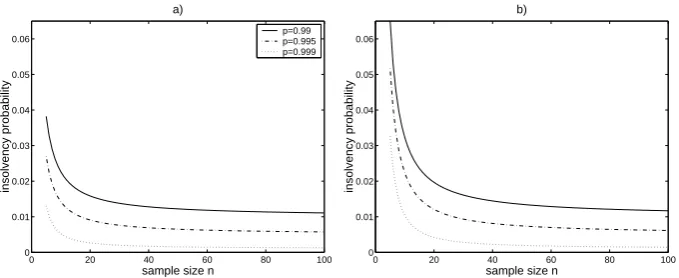
the size of the sample n. In figure 1a), the insolvency probability γ(p;θ) is
plotted against the sample sizenfor confidence levelsp= 0.99, 0.995, 0.999.
The following can be observed:
• The probability of insolvency is decreasing in the number of data points
n. This makes intuitive sense: the larger the sample, the higher the
accuracy of the capital assessment and thus the lower the probability
of insolvency.
• In particular as the sample size becomes very large, the insolvency probability tends to its required value 1−p, as can also be seen by
noting that limn→∞
[
1 +1nlog1−1p
]n
= exp
(
log1−1p
)
= 1−1p, so that limn→∞γ(p;θ) = 1−p.
• For small data sets, parameter error may cause the probability of in-solvency to be substantially higher than the required value; in that
sense a high confidence level quoted may be rather misleading in the
presence of parameter uncertainty. For example if n = 10 and p =
0.99, 0.995, 0.999the ratios of the true to the required probability of
in-solvency are γ1(0−.099;.99θ) = 00.023.01 = 2.26, γ1(0−.0995;.995θ) = 00..014005 = 2.85, γ1(0−.0999;.999θ) =
0.005
0.001 = 5.24.
Example 5. Suppose now that X1, . . ., Xn, Y are independent normal
N(µ, σ2) variables, so that θ = (µ, σ). The maximum likelihood estima-tors are µˆ = ∑nj=1Xj and σˆ2 = n−1
∑
(Xi −X¯)2, with σˆ independent of
ˆ
0 20 40 60 80 100 0
0.01 0.02 0.03 0.04 0.05 0.06
a)
sample size n
insolvency probability
p=0.99 p=0.995 p=0.999
0 20 40 60 80 100
0 0.01 0.02 0.03 0.04 0.05 0.06
b)
sample size n
insolvency probability
Figure 1: Probability of insolvency γ(p;θ) for a) exponentially and b)
normally distributed losses, against sample size n, for confidence levels
p= 0.99, 0.995, 0.999
V ∼χ2n−1, and V is independent ofU. The capital held is given byc(p,X) =
F−1(p; (ˆµ,σˆ)) = ˆµ+ ˆσΦ−1(p), where Φis the N(0,1)distribution function.
Now
Pθ[Y ≤c(p,X)] =Pθ[Y −µˆ≤σˆΦ−1(p)],
Observe thatY −µˆ∼N(0,n+1n σ2), independent of V, implying that
√ n n+ 1·
Y −µˆ
√
σ2V /(n−1) ∼tn−1.
In consequence,
γ(p;θ) =Tn−1
(√ n−1
n+ 1Φ
−1(p)
)
, (5)
where Tn−1(·) denotes the distribution of a tn−1 variable. In figure 1b) the
insolvency probability is again plotted as a function ofn, giving a very similar
pattern to that observed for the exponential distribution. Forn→ ∞we have
Tn−1→Φ so that again limn→∞γ(p;θ) =p.
2.2 Increasing transformations
Given that the confidence level p is generally chosen to be close to 1, the
solvency probabilityγ(p;θ) relates to the extreme tail of the loss distribution.
It may then be assumed that the overall shape and in particular the tail
properties of the loss distribution F(·;θ) have a substantial effect on the
[image:12.595.136.476.73.212.2]Such a relationship is not straightforward. To show this consider another
portfolio, for which the sample and future loss considered satisfy
X1∗=d h1(X1), . . . , Xn∗ d
=hn(Xn), Y∗ d
=h(Y),
where = denotes equality in distribution andd h1, . . . , hn, h are strictly
in-creasing functions not depending on the parameterθ.
It can then be easily shown (Lemma 2 in the Appendix) that the solvency
probabilities for the two portfolios are actually going to be the same, that
is:
Pθ[Y ≤F−1(p; ˆθ(X))] =Pθ[Y∗≤F∗−1(p; ˆθ(X∗))] (6)
Note that for a non-linear function h, the probability distributions of the
losses Y and Y∗ may have very different shapes, e.g. Y may be light-tailed
and/or symmetric, while Y∗ is heavy-tailed and/or skewed. Remarkably, the effect of parameter uncertainty on the solvency probability of those two
portfolios is the same. This is seen in the following example.
Example 6. Consider i.i.d. exponential losses X1, . . . , Xn, Y ∼ F(x;θ) =
1−e−xθ, x >0. Define now X∗
1, . . . , Xn∗, Y∗ ∼F∗(x;θ) = 1−x−
1
θ, x > 1
via the transformation h(t) = et. Therefore, X1∗, . . . , Xn∗, Y∗ follow a one-parameter Pareto distribution. The tail-behaviour of the Pareto distribution
is very different to that of the exponential distribution; in fact it is known
from extreme value theory[25] that the exponential and Pareto distributions
form limiting cases of the tails of light- and heavy-tailed distributions
respec-tively. Lemma 2 implies that for both these distributions the probability of
solvency γ(p;θ) will be the same, given by formula (4). This implies that
for the Pareto distribution the solvency probability is again independent of
the unknown parameter θ.
Similarly, for normally distributed losses X1, . . . , Xn, Y ∼ N(µ, σ2), by
applying the transformation h(t) =et we get a Lognormally distributed loss profile X1∗, . . . , Xn∗, Y∗. Again the Normal and Lognormal distributions are very different; the former is symmetric, has unbounded support and is
light-tailed, while the latter is skewed, has positive support and is heavy tailed
(in the sense of sub-exponentiality[25]). The formula (5) will apply to both distributions, so that the solvency probability for the Lognormal distribution
is again independent of the unknown parameters(µ, σ).
Hence the shape and heavy-tailedness of the loss distribution does not
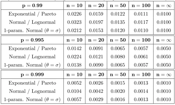
these probabilities is the number of unknown parameters in the distribution.
In Table I the insolvency probabilities γ(p;θ) for the Exponential/Pareto,
Normal/Log-normal models, as well as a one-parameter Normal model with
known mean, are compared for p = 0.99, 0.995, 0.999. It can be seen that
in all cases the 2-parameter Normal/Log-normal model produces a higher
probability of insolvency than the Exponential/Pareto one. This may be
at-tributed to the fact that the Normal/Log-normal model has an additional
lo-cation parameter, which exacerbates the effect of parameter uncertainty. On
the other hand, a 1-parameter Normal model, with only the variance (scale
[image:14.595.124.498.288.512.2]parameter) unknown, gives results very close to those of the exponential.
Table I: Comparison of insolvency probabilities γ(p;θ) for the
Exponen-tial/Pareto and Normal/Log-normal models (for p = 0.99, 0.995, 0.999).
p=0.99 n=10 n=20 n=50 n=100 n=∞ Exponential / Pareto 0.0226 0.0159 0.0122 0.0111 0.0100
Normal / Lognormal 0.0323 0.0197 0.0135 0.0117 0.0100
1-param. Normal (θ=σ) 0.0212 0.0153 0.0120 0.0110 0.0100
p=0.995 n=10 n=20 n=50 n=100 n=∞ Exponential / Pareto 0.0142 0.0091 0.0065 0.0057 0.0050
Normal / Lognormal 0.0224 0.0121 0.0080 0.0061 0.0050
1-param. Normal (θ=σ) 0.0138 0.0090 0.0065 0.0057 0.0050
p=0.999 n=10 n=20 n=50 n=100 n=∞ Exponential / Pareto 0.0052 0.0026 0.0015 0.0013 0.0010
Normal / Lognormal 0.0104 0.0042 0.0020 0.0014 0.0010
1-param. Normal (θ=σ) 0.0057 0.0029 0.0016 0.0013 0.0010
2.3 Independence of solvency probability from parameters
In the examples of Sections 2.1 and 2.2 it was seen that for particular
distri-butions it is possible to simply calculate the probability of solvency under
parameter uncertainty, since it does not depend on the unknown true
pa-rameters. In fact, this useful property holds not just for the special cases
considered, but for a wide class of probability distributions, including many
popular choices in risk modelling, that may be symmetric or asymmetric,
with bounded or unbounded support, light- or heavy-tailed.
The families of distributions we consider are 2-parameter transformed
location-scale families and 1-parameter transformed scale families. A
scale family if an increasing function of that random variable belongs to a
(location-) scale family. For example, if Y is exponentially distributed (a
scale family) then the random variable Y∗ = eY is Pareto distributed (a transformed scale family). A formal definition of transformed (location-)
scale families is given the Appendix. (Transformed location families can be
similarly defined and results similar to the ones derived later on for scale
and location-scale families hold. However these distributions are less useful
for loss modelling purposes and we will not be concerned with them here.)
Examples of location-scale families are the normal distribution, the
t-distribution, the logistic t-distribution, and the Laplace distribution. Such
distributions are commonly used in modelling asset log-returns [7],[26]. By lettingh(t) =et, we can derive from the distributions above, the log-normal, log-t, log-logistic (or Fisk) and log-Laplace distributions. Besides their
pos-sible use in asset return modelling these are popular models in modelling
heavy-tailed insurance or operational risk losses[27],[7]). It is simple to show that other popular loss distributions such as the two-parameter Weibull[24] can also be transformed to a (non-symmetric) location-scale family.
The simpler class of 1-parameter scale families includes the exponential
distribution, the Gamma and Weibull distributions (with shape parameter
fixed), or indeed any location-scale family with the location parameter fixed.
By transforming the exponential distribution via h(t) = et, we get the 1-parameter Pareto distribution, with cdf 1−x−1/θ, x >1. It is easy to see that the usual Pareto distribution 1−ba(b+x)−a also belongs to a transformed scale family if we keep either of the two parameters fixed.
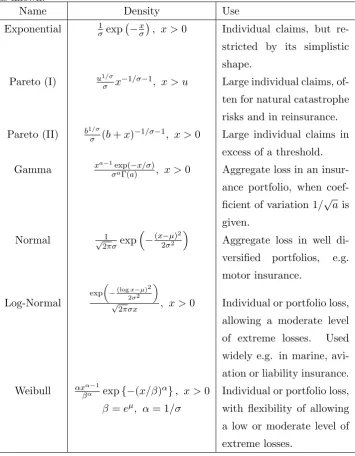
Some of these distributions and their uses in insurance loss modelling
are summarised in Table II.
We then have the following result, stated as Proposition 1 in the
Ap-pendix. If the probability distributions of the dataF1(·;θ), . . . , Fn(·;θ) and
of the future loss F(·;θ) belong to a transformed (location-) scale family,
capital is calculated by an estimated loss percentile as in equation (2), and
the parameter(s)θare estimated via maximum likelihood, the corresponding
probability of insolvencyγ(p;θ) does not depend on the true parameter(s)θ.
Therefore, for a wide range of useful loss models it is possible to determine
Table II: Distributions in transformed (location-)scale families that are
com-monly used in insurance loss modelling. Location and scale parameters are
denoted byµ, σ respectively; parameters otherwise denoted are considered
as known.
Name Density Use
Exponential σ1exp(−xσ), x >0 Individual claims, but re-stricted by its simplistic
shape.
Pareto (I) u1σ/σx−1/σ−1, x > u Large individual claims, of-ten for natural catastrophe
risks and in reinsurance.
Pareto (II) b1σ/σ(b+x)−1/σ−1, x >0 Large individual claims in excess of a threshold.
Gamma xa−1σexp(aΓ(a−)x/σ), x >0 Aggregate loss in an
insur-ance portfolio, when
coef-ficient of variation 1/√ais
given.
Normal √1
2πσexp
(
−(x−µ)2 2σ2
)
Aggregate loss in well
di-versified portfolios, e.g.
motor insurance.
Log-Normal
exp
(
−(logx−µ)2 2σ2
)
√
2πσx , x >0 Individual or portfolio loss,
allowing a moderate level
of extreme losses. Used
widely e.g. in marine,
avi-ation or liability insurance.
Weibull αxβαα−1 exp{−(x/β)α}, x >0 Individual or portfolio loss,
β=eµ, α= 1/σ with flexibility of allowing a low or moderate level of
extreme losses.
2.4 Numerical calculation of solvency probability
Exact calculation of the probability of solvency can be surmised from
Propo-sition 1 in the Appendix. However, such calculation requires integration
with respect to the density of the estimator, which is not generally known
in closed form. However, the solvency probability can always be calculated
Section 2.1. The simulation of different loss histories can take place forany
choice of parameters, for example by setting the location and scale
param-eters to 0 and 1 respectively; Proposition 1 guarantees that the choice of
parameters will not affect the result. The following example illustrates the
process.
Example 7. Consider i.i.d. X1, . . . , Xn∼F(·;θ) where F(·;θ), θ= (µ, σ),
is a Weibull distribution such that
F(x;θ) = 1−exp
{
−(e−µx)1/σ }
, x >0.
The Weibull distribution is a popular choice for modelling insurance losses,
as it can represent a range of tail-behaviour, depending on the choice of
shape parameterσ (orα= 1/σin a more usual parameterisation[27]). The
increasing transformation Xi∗ = logXi, Y∗ = logY yields random variables
following a negative Gumbel distribution
F∗(x;θ) = 1−exp
{ e−x−σµ
} .
The Gumbel distribution is a location-scale family, hence Proposition 1
ap-plies and the probability of solvency γ(p;θ) does not depend on the true
parametersθ= (µ, σ).
There is no explicit formula for Maximum Likelihood Estimator (MLE) ˆ
θ= (ˆµ,σˆ) of θ, which is given as the solution to the system of equations
nˆσ+∑nj=1log(e−µˆXj
)
−∑n j=1
( e−µˆXj
)1/ˆσ
log(e−µˆXj
) = 0 ( 1 n ∑n j=1X
1/σˆ
j
)ˆσ
−eµˆ = 0 (7)
It has been shown that in estimating parameters for the Gumbel distribution
using small samples, the MLE is outperformed (in the Mean-Squared-Error
sense) by estimators based on Probability Weighted Moments (PWM)[28],[29]. PWM estimators are also computationally simpler to evaluate, giving
for-mulas ˜ σ = 2 n n ∑ j=1
j−1
n−1Xj:n−X¯
/log 2, µ˜= ¯X+γ˜σ, (8)
where X¯ is the sample mean, X1:n ≤ X2:n ≤ · · · ≤ Xn:n are the order
statistics and γ ≃0.57721 is the Euler constant. The estimators (8),
simi-larly to MLE, satisfy an equivariance property (in the sense of Lemma 3 in
the Appendix), which means that Proposition 1 still holds and the solvency
The required capital is then calculated as
c(p;X) =e−m(−log(1−p))s, (9)
by setting either(m, s) = (ˆµ,σˆ) or (m, s) = (˜µ,σ˜).
Hence the following algorithm can be used to calculate γ(p;θ) using a
Monte-Carlo sample of size r:
• Loop from i= 1 to i=r
– Generate i.i.d. observations (xi,1, . . . , xi,n, yi) from F(·; (0,1)).
– Estimateµ, σ by (7) or (8).
– Calculate capital c(p;xi) by (9).
– Record a ‘success’ ifc(p;xi)≥yi.
• Estimateγ(p;θ) as the number of successes divided by r.
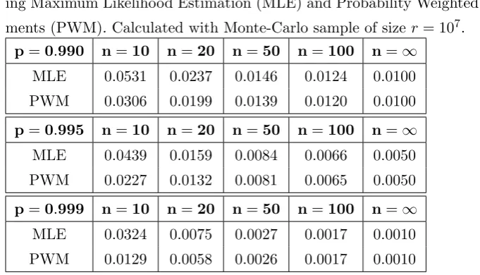
The algorithm was used in order to calculate the insolvency
probabil-ity ¯γ(p;θ) for confidence levels p= 0.99,0.995,0.999 and sample sizes n=
10,20,50,100. The calculation was carried out using a Monte-Carlo sample
of sizer= 107 and parameters were estimated with both the MLE and PWM methods. Results are summarised in Table III. Under PWM estimation, the
insolvency probabilities for the Weibull distribution are very close to those
of the 2-parameter (Log)normal distribution in Table I. However, for small
samples, the probability of insolvency is substantially higher when MLE is
used. This is explained by the worse performance of MLE compared to PWM
for the Gumbel/Weibull distribution, that has been observed [28],[29].
In-tuitively, less accurate parameter estimates are more likely to give rise to
inappropriate capital estimates and hence exacerbate the effect of
parame-ter uncertainty. The example indicates that weaknesses in the estimation
Table III: Insolvency probabilities γ(p;θ) for the Weibull distribution,
us-ing Maximum Likelihood Estimation (MLE) and Probability Weighted
Mo-ments (PWM). Calculated with Monte-Carlo sample of sizer= 107. p=0.990 n=10 n=20 n=50 n=100 n=∞
MLE 0.0531 0.0237 0.0146 0.0124 0.0100
PWM 0.0306 0.0199 0.0139 0.0120 0.0100
p=0.995 n=10 n=20 n=50 n=100 n=∞ MLE 0.0439 0.0159 0.0084 0.0066 0.0050
PWM 0.0227 0.0132 0.0081 0.0065 0.0050
p=0.999 n=10 n=20 n=50 n=100 n=∞ MLE 0.0324 0.0075 0.0027 0.0017 0.0010
PWM 0.0129 0.0058 0.0026 0.0017 0.0010
3
ADJUSTING THE CAPITAL REQUIREMENT
It was argued in Section 2 that, when capital is held equal to an estimated
percentile of the loss distribution, the solvency probability for the loss
port-folio is generally lower than the specified confidence level, due to the effect
of parameter uncertainty. Formally,
γ(p;θ) =Pθ[Y ≤F−1(p; ˆθ)]≤Pθ[Y ≤F−1(p;θ)] =p.
Such a situation is of course unsatisfactory, since the true probability of a
portfolio being solvent can be substantially lower than the one required by,
for example, a regulator or the holder’s own risk management.
In this section we explore two methods for adjusting the capital
require-ment, in order to reflect the effect of parameter uncertainty on solvency and
thus increase the solvency probability to its required level. In both methods
the capital requirement becomes higher. The first one relies on raising the
confidence level of the solvency capital calculation, while the second one,
based on Bayesian arguments, adjusts the probability distribution used for
capital setting.
3.1 Raising the confidence level
One could address the problem of the solvency probability being lower than
its specified level, by setting the capital at a higher confidence level, that is,
require that capital is set by:
The adjusted confidence levelp∗ could then be selected by requiring that
γ(p∗;X) =Pθ[Y ≤c(p∗;X)] =p (10)
If the loss distributionF(·;θ) belongs to a transformed (location-) scale
fam-ily, the probability of solvency does not depend on the unknown parameter
θ. Hence we can explicitly solve equation (10) and specify the adjusted
confidence levelp∗. The process is illustrated in the following example.
Example 8. Let as before X1, . . . , Xn, Y distributed according to an
expo-nential or one-parameter Pareto distribution. Then it was shown in Example
4 that the solvency probability is given by:
γ(p;θ) = 1−
[
1 + 1
nlog
1 1−p
]−n
We require
γ(p∗;θ) =p =⇒ p∗= 1−exp
{
−n [
(1−p)−1/n−1
]}
Therefore the confidence level according to which the capital has to be
calcu-lated becomes a function of the size n of the dataset. This is demonstrated
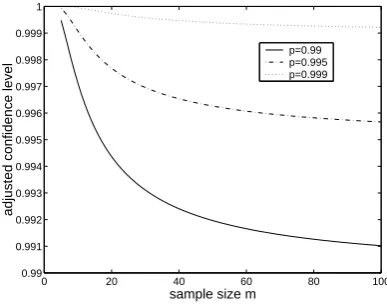
in figure 2, where the value of p∗ is plotted against n for different values of the required solvency levelp= 0.99, 0.995, 0.999. It can be seen that p∗ de-creases as the sample sizengets larger, so thatp∗→pasn→ ∞. Hence the
holder of a portfolio with a long history of relevant data will have to calculate
its capital according to a confidence level close to the required solvency
prob-ability p. In contrast, the holder of a portfolio for which very few observed
data exist will have to set capital according to a confidence level that is much
higher than p. For example, for n = 10 we have p = 0.99 ⇒ p∗ = 0.9971,
p= 0.995⇒p∗= 0.9991, p= 0.999⇒p∗ = 0.99995.
Following the approach suggested here, each loss portfolio will have to
be assigned a different confidence levelp∗, on which the capital requirement
is based, where p∗ depends on the loss distribution and the sample size for the portfolio. On the face of it this makes sense: long experience and
diligent data collection are rewarded with a lower capital requirement; lack of
experience and incomplete data are penalised. It is noted that this argument
refers torelevant experience. It may be that a company has a long history
but changes in the risk profile, e.g. due to changes in portfolio mix or perils
0 20 40 60 80 100 0.99
0.991 0.992 0.993 0.994 0.995 0.996 0.997 0.998 0.999 1
sample size m
adjusted confidence level
[image:21.595.207.401.74.226.2]p=0.99 p=0.995 p=0.999
Figure 2: Adjusted confidence levelp∗ used for capital setting in the expo-nential/Pareto model, as a function of sample size n, for required solvency
probabilitiesp= 0.99, 0.995, 0.999
not deal with the case of detecting distributional changes over time, and
assume throughout that the data used are i.i.d.; discarding irrelevant data
of course reduces the sample size andincreases the capital requirement.
There are other problems with adopting such an approach in practice
too. Consider that the capital requirement is being set by a regulator. This
means that the regulator would have to set a different confidence level p∗
for each regulated risk portfolio. Therefore the regulator would have to be
equipped with the knowledge of each portfolio’s aggregate loss distribution
(assuming this belongs to a transformed location-scale family), so thatp∗can
be calculated. Gathering such information may be logistically challenging
and assumes that regulators would be much closer to insurance company’s
modelling than they really are. Moreover, such an approach may appear
excessively prescriptive and thus at odds with principles-based regulatory
regimes such as ICAS and Solvency II.
Furthermore, such capital setting would likely be challenged by the
port-folio holders. The adoption of different confidence levels across portport-folios
would give the impression of inequity and may be politically difficult to
sup-port. Implementation of the regime would not be helped by the potential
difficulty of explaining it to portfolio holders. The adjustment to the
con-fidence level relies on the rather abstract notion of a random capital level,
as in equations (2), (3). As discussed in Section 2.1, this may be best
ex-plained as an expected frequency of solvency across portfolios. While such
necessarily relevant to individual portfolio holders such as insurance firms.
After all, the idea of a random capital level may strike portfolio holders, who
have already observed past losses and set their capital at a fixed amount,
as rather odd. Of course, no regulator would communicate in such abstract
terms, but instead state that a higher requirement is due whenever there
is insufficient information about the loss distribution. While this may help
communication, it would not resolve the underlying epistemic problem.
The next section proposes an adjusted capital requirement that addresses
these issues.
3.2 Adjusting the loss distribution
If holders of risk portfolios find the frequentist interpretation of parameter
uncertainty used to justify the adjustment in Section 3.1 meaningless, a
dif-ferent conceptualisation of uncertainty is necessary. This can be achieved
using standard Bayesian arguments. Unknown parameters can be
consid-ered as random quantities and the additional risk to solvency induced by
parameter uncertainty can be reflected by constructing a more dispersed
predictive distribution.
A prior densityπ(θ) is defined over the parameter spaceθ∈ S. The prior
π is potentially improper and can be chosen to be uninformative, so that
subjective judgement does not enter the calculation. Given the observed
dataX=x, the parameters’ posterior density is given by:
π(θ|x) =I(x)−1π(θ)
n
∏
j=1
fj(xj;θ), (11)
whereI(x) =∫η∈Sπ(η)∏jn=1fj(xj;η)dη. The predictive density and
distri-bution ofY are respectively defined as:
ˆ
f(y|x) =
∫
η∈S
f(y;η)π(η|x)dη, Fˆ(y|x) =
∫
η∈S
F(y;η)π(η|x)dη. (12)
Probabilities calculated using the predictive density are denoted by ˆP(·|x). An alternative way of raising the capital requirement is then, rather than
increase the confidence level, to adjust the loss distribution used for capital
setting by using the predictive distribution. This reflects parameter
uncer-tainty by being typically more dispersed than the loss distributionF(·; ˆθ(x)).
Thus capital can be set as a percentile of the predictive distribution:
ˆ
Such an approach presents substantial practical advantages compared to
the adjustment of the confidence level discussed in Section 3.1. A regulatory
regime whereby capital is set as a percentile of the predictive distribution is
consistent with principle-based regimes; the regulator has only to specify a
confidence level, the same for all companies, and all calculations are carried
out by companies themselves. The regulator does not need to have access
to loss data or to know the family of loss distributions best describing the
portfolio’s loss profile. In effect, the change from current regulatory practices
would be marginal; rather than the regulator saying ‘calculate your capital
requirement as the 99.5th percentile of your estimated loss distribution,”
he would say ‘calculate your capital requirement as the 99.5th percentile
of your predictive loss distribution.” Furthermore, from the perspective of
portfolio holders, reflecting parameter uncertainty by defining a distribution
over the parameters may be easier to interpret than viewing the capital held
as a random number.
It is, however, not clear whether setting capital by the predictive
dis-tribution has the desired effect, that is, whether it raises the probability of
solvency, with respect to the true parameters, to an acceptable level. That
is, we would like to know the value of the probability:
δ(p;θ) =Pθ[Y ≤cˆ(p|X)], (14)
where the capital level ˆc(p|X) is now viewed as a random variable.
Essen-tially (14) states the expected probability of solvency from the perspective
of a regulator, when the capital is set according to (13). Ideally it would
beδ(p;θ) =p, as it would mean that the adjustment to the capital setting
regime raised the probability of solvency to its required level. An example
where such consistency holds is given next.
Example 9. Let i.i.d. X1, . . . , Xn, Y follow F(x;θ) = 1−e−
x
θ, x ≥ 0.
Standard arguments show that for prior π(θ) = θ−ν, ν ≥ 0 and observed sampleX=x, the predictive distribution obtained is
ˆ
f(y|x) = (n+ν−1) (
∑
jxj)n+ν−1
(y+∑jxj)n+ν ⇒
ˆ
P[Y > y|x] =
( ∑
jxj
y+∑jxj
)n+ν−1
,
which is a Pareto distribution; hence the allowance for parameter uncertainty
has turned the distribution used for capital assessment from a light- to a
heavy tailed one. Capital can then be set as:
ˆ
c(p|x) = ˆF−1(p|x) =∑
j
xj
[
(1−p)−1/(n+ν−1)−1
The expected frequency of insolvencies under this capital setting method is
given by
δ(p;θ) = Pθ[Y >ˆc(p|X)]
= Pθ
Y >∑
j
Xj
(
(1−p)−1/(n+ν−1)−1
)
= Pθ
[ ∑
jXj
∑
jXj+Y
<(1−p)1/(n+ν−1)
] .
The quantity
∑
jXj
∑
jXj+Y follows aBeta(n,1)distribution with cumulative
dis-tributionB(x;n,1) =xn, x∈[0,1]. Therefore
δ(p;θ) = (1−p)n/(n+ν−1) (15)
Note that if we let ν = 1, that is, if we use an uninformative prior of the
formπ(θ) =θ−1 appropriate for scale families[30], we get
δ(p;θ) = 1−p⇔δ(p;θ) =p,
as required.
The example demonstrated the potential effectiveness of using a
pre-dictive distribution for capital setting, in satisfying the regulatory solvency
probability requirement. Such consistency between Bayesian and frequentist
methods[24],[22]is more generally true for the transformed (location-) scale families discussed in this paper. In particular, as shown in Proposition 2 in
the Appendix, for such distributions, when the priorπ(µ, σ) =σ−1 is used, it is always the case that δ(p;θ) =p. More broadly, for priors of the form
π(µ, σ) =σ−ν, we find that the resulting solvency probability again does not depend on the real parameters, so that the probability can be potentially
calculated by a regulator.
4
DATA POOLING
In Section 3 it was argued that the effect of parameter uncertainty on
sol-vency can be addressed by a stricter regulatory regime, adopting a higher
confidence level or more dispersed loss distribution. These are actions that
a regulator may take. Portfolio holders on the other hand can increase their
probability of solvency by addressing the key issue discussed in this paper:
We assume that the losses from the portfolios of a number of different
companies, follow distributions with the same parameters, after appropriate
adjustments. (This simplifying assumption is of course quite strong. We
are not concerned here with credibility theory, the optimal combined use of
a company’s own and benchmark data for pricing purposes[27], which has also been proposed in the context of operational risk capital setting [31]).
Then the portfolio holders may decide to pool their data in order that each
of them is able to estimate their required capital from a larger data set. As
a consequence the solvency probability of each should increase.
We note that the setting here is somewhat contrived, as it is required
that companies have independent risk exposures following similar probability
distributions, which are estimated using the same benchmark data set. This
is a situation not easily envisaged in insurance risk management. However in
operational risk management, pooling of loss data between different financial
institutions does occur [32], while it is not unreasonable to assume that operational risk losses are independent across institutions.
A side-effect of pooling data is that, even if the losses from different
port-folios are independent, the portfolio (in)solvency events become dependent.
This is because the capital of each portfolio is calculated on the basis of the
same random sample. Hence there is a chance that the capital is collectively
over- or under-stated for all portfolios. One has to then examine the effect
of data sharing on systemic stability, for example via the joint probability
of insolvency. Such an examination is given below, for the simple example
of two portfolios with exponentially distributed losses. The process can be
carried out for losses in any (location-) scale family, as the joint insolvency
probability will again be independent of the true parameterθ.
Example 10. Consider the simple case where only two portfolios exist, and all losses, within and across portfolios, are i.i.d. Hence we have
X1 = (X1,1, . . . , X1,n1), Y1
X2 = (X2,1, . . . , X2,n2), Y2 }
∼F(·;θ),
where F is an exponential or Pareto distribution. Let X = (X1,X2) and
n = n1 +n2. First consider the case that data are not pooled. Then the
probability of insolvency for each portfolio is
Pθ[Yi > c(pi;Xi)] =
[
1 + 1
ni
log 1 1−pi
]−ni
and the joint probability of insolvency is given by:
Pθ[Y1 > c(p1;X1), Y2> c(p2;X2)] =
[
1 + 1
n1
log 1 1−p1
]−n1[
1 + 1
n2
log 1 1−p2
]−n2 .
(16)
Let now the two portfolios merge their data sets. Then the probability of
insolvency for each portfolio is
Pθ[Yi > c(p;X)] =
[
1 + 1
nlog
1 1−pi
]−n
, i= 1,2,
which is lower than Pθ[Yi > c(pi;Xi)], demonstrating the beneficial effect of
data sharing. Calculation yields the joint probability of insolvency as
Pθ[Y1> c(p1;X), Y2 > c(p2;X)] =
[
1 +1
nlog (
1
(1−p1)(1−p2)
)]−n
.
(17)
So which of the two situations (pooled or un-pooled data) produces a lower
joint probability of insolvency? Observe that
Pθ[Y1 > c(p1;X), Y2> c(p2;X)]−1/n= 1 +
1
nlog (
1
(1−p1)(1−p2)
) = 1 n [ n1 (
1 + 1
n1
log 1 1−p1
)
+n2
(
1 + 1
n2
log 1 1−p2
)]
≥
[(
1 + 1
n1
log 1 1−p1
)n1(
1 + 1
n2
log 1 1−p2
)n2]1/n
=Pθ[Y1 > c(p1;X1), Y2 > c(p2;X2)]−1/n,
(where the inequality follows from the fact that the arithmetic mean is greater
than the geometric one) implying
Pθ[Y1 > c(p1;X), Y2> c(p2;X)]≤Pθ[Y1 > c(p1;X1), Y2> c(p2;X2)]
Note that an equality is obtained only for n1log(1−p1) = n2log(1−p2);
in particular when p1 = p2 we have equality for n1 = n2. In this simple
example, pooling of data is beneficial at the individual portfolio, as well as
the systemic level.
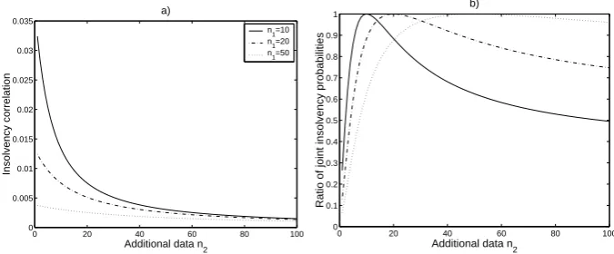
For a numerical example we fix p1=p2 = 0.995and letn1 = 10, 20, 50.
In figure 3a) we plot against n2 the correlation of the indicator functions
of insolvency events {Y1 > c(p1;X)}, {Y2 > c(p2;X)}. This ‘insolvency
event correlation’ is similar to the default correlation encountered in credit
risk analysis [7]. It can be seen that the correlation is positive, indicating
0 20 40 60 80 100 0
0.005 0.01 0.015 0.02 0.025 0.03 0.035
Additional data n
2
Insolvency correlation
a)
n1=10
n
1=20
n1=50
0 20 40 60 80 100
0 0.1 0.2 0.3 0.4 0.5 0.6 0.7 0.8 0.9 1
Additional data n
2
Ratio of joint insolvency probabilities
[image:27.595.135.473.76.216.2]b)
Figure 3: The effect of pooling on joint insolvency, for exponential/Pareto
losses, n1 = 10, ,20, 50 and p1 = p2 = 0.995: a) insolvency event
corre-lation; b) ratio of the joint insolvency probabilities Pθ[Y1 > c(p1;X), Y2 >
c(p2;X)]/Pθ[Y1> c(p1;X1), Y2 > c(p2;X2)].
is reduced when the number of available data n1, n2 increases. In figure
3b), the ratio of the joint insolvency probabilities Pθ[Y1 > c(p1;X), Y2 >
c(p2;X)]/Pθ[Y1 > c(p1;X1), Y2 > c(p2;X2)] is plotted. It is seen that the
ratio is always < 1, such that data pooling, while introducing insolvency
correlation, does not increase systemic risk. The lowest values of the ratio
are obtained whenn1andn2are very different. This implies that the greatest
benefit of pooling data is obtained when, of the two data-sets pooled, the one
is small and the other large.
5
CONCLUSION AND DISCUSSION
In the article it is argued that a frequentist interpretation of parameter
un-certainty is appropriate for quantifying its effect on the solvency probability
of loss portfolios, when seen through the eyes of a regulator. It is shown that
for a rich class of loss distributions, solvency probabilities can be explicitly
calculated (even though the real parameters remain unknown) and depend
strongly on the size of the data set used for the estimation of risk capital. In
particular we show that for small datasets the true probability of insolvency
for a portfolio can be much higher than the notional one. When taking
the viewpoint of a financial firm, a Bayesian interpretation of uncertainty
is more appropriate. Hence we propose an improvement on current capital