S 0033-569X(2011)01265-5
Article electronically published on September 7, 2011
KICKBACK IN NEMATIC LIQUID CRYSTALS
By
F. P. DA COSTA (Departamento de Ciˆencias e Tecnologia, Universidade Aberta, Rua da Escola
Polit´ecnica, 141, P-1269-001 Lisboa, Portugal, and Center for Mathematical Analysis, Geometry and Dynamical Systems, Instituto Superior T´ecnico, TU Lisbon, Av. Rovisco Pais, 1, P-1049-001 Lisboa,
Portugal),
M. GRINFELD (Department of Mathematics and Statistics, University of Strathclyde, Glasgow G1
1XH, United Kingdom),
M. LANGER (Department of Mathematics and Statistics, University of Strathclyde, Glasgow G1
1XH, United Kingdom),
N. J. MOTTRAM (Department of Mathematics and Statistics, University of Strathclyde, Glasgow
G1 1XH, United Kingdom),
and
J. T. PINTO (Departamento de Matem´atica, Instituto Superior T´ecnico, TU Lisbon, Av. Rovisco
Pais, 1, P-1049-001 Lisboa, Portugal, and Center for Mathematical Analysis, Geometry and Dynamical Systems, Instituto Superior T´ecnico, TU Lisbon, Av. Rovisco Pais, 1, P-1049-001 Lisboa,
Portugal)
Abstract. We describe a nonlocal linear partial differential equation arising in the analysis of dynamics of a nematic liquid crystal. We confirm that it accounts for the kick-back phenomenon by decoupling the director dynamics from the flow. We also analyse some of the mathematical properties of the decoupled director equation.
1. Introduction. Consider a thin layer of nematic liquid crystalline fluid sandwiched between two parallel glass plates separated by a gap of width 2d. Suppose it is subjected to a large magnetic field aligned in the direction normal to the plates. The dynamics of the solution is then essentially one dimensional [13], and is well described by the director angleθ(z, t), which is the average angle a rod-like nematic liquid crystal molecule forms with the plane of the plates, and by the flow speed v(z, t) parallel to the plates. Here z ∈(−d, d) is the coordinate in the direction of the normal. We assume that the
Received June 10, 2010.
2000Mathematics Subject Classification. Primary 34D15, 35Q72; Secondary 76A15, 82D30.
Key words and phrases. Nematic liquid crystals, kickback, singular perturbations, nonlocal operators. E-mail address:[email protected]
E-mail address:[email protected]
E-mail address:[email protected]
E-mail address:[email protected]
E-mail address:[email protected]
c
2011 Brown University
system is strongly anchored, which means that for all timet,θ(−d, t) =θ(d, t) = 0 and
v(−d, t) =v(d, t) = 0. Suppose that, with the magnetic field applied, we allow the system to reach equilibrium. At equilibrium, for large magnitudes of the applied magnetic field, apart from a transition layer close to the glass plates, the director is aligned to the magnetic field, so that in the bulk θ(z, t)≈π/2, as we show later. Now suppose that, say, att= 0, we switch off the magnetic field.
The equations governing the dynamics of the director and the flow speed after the magnetic field is turned off [13, pp. 225–226] are
γ1θt =
K1cos2θ+K3sin2θ
θzz
+ (K3−K1) sinθcosθ(θz) 2
−m(θ)vz, (1.1) ρvt = (g(θ)vz+m(θ)θt)z, (1.2)
where
m(θ) = α3cos2θ−α2sin2θ, (1.3)
g(θ) = 1 2
α4+ (α5−α2) sin2θ+ (α3+α6) cos2θ
+α1sin2θcos2θ, (1.4)
γ1 andαi are various viscosities,Kj are elastic constants, andρis the fluid density.
The (Ericksen–Leslie) equations (1.1)–(1.2) are supplemented with homogeneous Di-richlet boundary conditions and initial conditions forθandv. For the director angle the initial condition isθ(z,0) =θ0(z), whereθ0(z) is the solution of the quasilinear field-on equilibrium equation, which is [13]
(K1cos2θ0+K3sin2θ0)θ0zz+ (K3−K1) sinθ0cosθ0(θ0z) 2
(1.5)
+ μ0ΔχH2sinθ0cosθ0 = 0,
whereH is the magnitude of the magnetic field,μ0is the permeability of free space, Δχ is the magnetic anisotropy, andθ0(±d) = 0. Since we have assumed that the magnetic field has been applied for a sufficiently long time to achieve equilibrium, the fluid will be stationary just before we switch the field off. We therefore take the initial condition for the fluid speed to bev(z,0)≡0.
If we now perform the rescaling (z, t)→(x, s) by letting
z=d x, t=τ1s, (1.6)
introducing ˆθ(x, s) =θ(z, t) and ˆv(x, s) =v(z, t), and the new constant parameters
λ:=−α2d
K3
, ζ:= γ1d
K3
, τ1:=
d2γ1
K3
, τ2:=−
d2ρ α2
, k:= K1
K3
, (1.7)
the problem (1.1)–(1.2) becomes
ˆ
θs =
kcos2θˆ+ sin2θˆ
ˆ
θxx
+ (1−k) sin ˆθcos ˆθ
ˆ
θx 2
+ ˆm(ˆθ) (λˆvx), (1.8) τ2
τ1
(ζvˆs) =
−ˆg(ˆθ) (ζˆvx)−mˆ(ˆθ)ˆθs
where
ˆ
m(ˆθ) = a3cos2θˆ−sin2θ,ˆ (1.10)
ˆ
g(ˆθ) = 1 2
a4+ (a5−1) sin2θˆ+ (a3+a6) cos2θˆ
+a1sin2θˆcos2θ,ˆ (1.11)
andai =αi/α2 fori= 1,3,4,5,6. The parameterkis a measure of the deviation from elastic isotropy and is often taken to be one in order to simplify the equations. We will not need to use this simplification in this paper.
The parameters λand ζ have dimensions of the inverse of velocity and provide two fluid velocity scales. The first velocity scale 1/λ derives from the flow induced by the reorientation of the director due to the elastic effects and, as can be seen in equation (1.7), the second, 1/ζ, is simply a rescaling of the first by the ratio of viscosities−γ1/α2. (Note thatγ1>0 andα2<0 for liquid crystals consisting of elongated rod-like molecules. For liquid crystals consisting of disc-like molecules α2 >0 and the obvious changes of sign in parameters such asλwould be used.)
There are also evidently two time scales in this problem,τ1andτ2. The first time scale,
τ1, with which we have rescaled time, is the typical time for elastic effects to reorient the director. The second time scale,τ2, is the time scale at which the fluid inertia reacts to changes in director orientation. In a standard liquid crystalline material these two time scales are considerably different. For example, in the liquid crystal 5CB, using the parameter values provided in [13, Appendix D], and assuming we have a liquid crystal layer of thicknessd= 1×10⁻⁵m (a typical device thickness) we find
τ1= 0.948 s, τ2= 1.256×10⁻⁶s. (1.12) Because of the vast difference in time scales of these two effects, which mean thatτ2/τ1 is significantly smaller than 1, it is common to neglect the inertial term in equation (1.9). This can be justified in a formal way using a multiple time scale analysis [15], and it is found that, on the time scale of director reorientationτ1, the velocity field is essentially a “slave” variable to the director angle. On this time scale, which is the one we are interested in, the simplified equations are then
ˆ
θs =
kcos2θˆ+ sin2θˆ
ˆ
θxx
+ (1−k) sin ˆθcos ˆθ
ˆ
θx 2
+ ˆm(ˆθ) (λˆvx), (1.13)
0 =
ˆ
g(ˆθ) (ζvˆx) + ˆm(ˆθ)ˆθs
x. (1.14)
On this time scale the time s = 0 is in fact the time after which the velocity has re-configured, through inertia effects, to allow equation (1.14) to be satisfied. Therefore, although the initial condition for ˆθ(x,0) = ˆθ0(x) remains the one obtained from the field-on governing equation (1.5) appropriately rescaled using equation (1.6), the initial condition for the flow speed must be altered and is obtained by solving (1.13) ats= 0 for ˆθs and then solving (1.14) for ˆv. However, the procedure we suggest in this paper
makes this unnecessary.
middle of the layer, before decaying to the rest state ˆθ(x, s)≡ 0; see for example [12, Fig. 11]. It was first described under the name of “optical bounce” in the experimental literature [6, 14, 1] in the mid-1970s and analysed in [2]. We would like to explain the observed dynamics of the early stages of kickback, from which experimentalists obtain information about the physical properties of the liquid crystal. The very complex and time-consuming procedure of fitting optical measurements to numerical solutions of (1.1)– (1.2) is described in [3, 12].
Certainly, it is difficult to see how to analyse (1.13)–(1.14) other than by numerical methods. However, a different approach [2] is as follows: for largeH, the director aligns with the magnetic field direction, and ˆθ0(x) is exponentially close to π/2 in the bulk. Hence for s >0 sufficiently small, the dynamics in the bulk (i.e., away from boundary layers) is well described by evaluating the nonlinear terms in (1.1)–(1.2) at ˆθ = π/2,
which gives
ˆ
θs= ˆθxx−λˆvx,
0 = ˆvxx+βθˆxs,
(1.15)
for s > 0 and |x| < 1, and where we have defined the nondimensional parameterβ = −α2/(ζη2) withη2= (α4+α5−α2)/2, which is a Miesowicz viscosity and always positive. These equations are subjected to the boundary conditions
ˆ
θ(−1, s) = ˆθ(1, s) = 0, vˆ(−1, s) = ˆv(1, s) = 0, fors >0, (1.16)
and the initial condition remains as ˆ
θ(x,0) = ˆθ0(x), for|x|<1. (1.17) Using (1.7) and the thermodynamical restrictions referred to in [13, page 230], it also follows that
λβ= α 2 2
η2γ1
∈(0,1). (1.18)
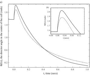
The approximation used above, thatθ0 ≈π/2, perhaps needs some further justifica-tion. In the bulk of the liquid crystal the alignment with the magnetic field means that this will be an acceptable approximation. However, we have insisted that ˆθ(±1, s) = 0 so that this approximation cannot be accurate close to the boundaries. For sufficiently long times the effects of these boundary conditions will surely be transmitted (through elastic relaxation) into the bulk of the cell. The question is, will kickback occur before the error in this approximation becomes apparent in the bulk of the liquid crystal? No analysis of this question will be considered in this paper, and it remains an interesting open problem. Instead we simply provide numerical evidence which justifies this approach for a standard liquid crystal. In Figure 1 we have numerically solved the system based on the nonlinear equations (1.13)–(1.14) as well as the system based on their linear counterparts (1.15), i.e., where the equations were “frozen” using the assumption that nonlinear terms are evaluated using ˆθ=π/2. We have used the material parameters for the liquid crystalline material 5CB (values taken from [13]) and the magnetic field value of H = 107A/m (equivalent to approximately 12 Tesla). Figure 1 shows that fort <0 the director angle in the middle of the cell is π/2 and increases when the magnetic field is removed (at
θ
(0,t), the director angle in the centre of the cell (rads)
t, time (secs)
t (secs)
θ
(0,t) (rads)
(a)
(b)
0.0 0.2 0.4 0.6 0.8 1.0
0.2 0.6 1.0 1.4 1.8
0.00 0.04 0.08 0.12 1.6
1.7 1.8 1.9 2.0
[image:5.612.159.457.121.371.2]-0.04
Fig. 1. Comparison between nonlinear (dashed) and linear (solid)
solutions: the director angle at the middle of the cellθ(0, t) as a function of time. For both cases we have neglected inertia. (b) is a zoomed plot of (a), close to when the magnetic field was turned off.
bulk” approximation has not qualitatively affected the kickback effect and in fact makes very little difference quantitatively. If we useθn(z, t) andθl(z, t) to denote the nonlinear
and linear solutions, respectively, and we letTnandTlbe the time for which the director
angle reaches its maximum for the two cases, then the time of maximum kickback has been changed by 1.2%, i.e., (Tn−Tl)/Tn= 0.012, and the maximum director angle value
is reduced by 7.9%, i.e, (max(θn(0, t))−max(θl(0, t)))/max(θn(0, t)) =−0.079. Given
that these are typical parameters for a liquid crystal cell, we are confident that the linear approximation will not overly affect the analysis in this paper.
2. Decoupling. We can now decouple the equations in (1.15). First, let us integrate the first equation in (1.15) with respect toxfrom −1 to 1 and use (1.16) to get
1
−1
θsdx= 1
−1
θxxdx. (2.1)
In (2.1) thev term disappears due to the boundary conditionsv(−1) = 0 =v(1). If we now integrate the second equation in (1.15) with respect toxfrom−1 tox, we obtain
vx(x, s)−vx(−1, s) =−βθs(x, s), (2.2)
where the boundary conditionθ(−1) = 0 (which implies thatθs(−1) = 0) has been used
to simplify the right-hand side.
Substitutingvx(x, s) from (2.2) into the first equation of (1.15) gives
μθs=θxx−λvx(−1, s). (2.3)
By (1.18),
μ≡1−λβ >0, (2.4)
and we will show below that this condition is sufficient for well-posedness of (2.3). If we then integrate equation (2.3) from−1 to 1, we obtain
μ 1
−1
θsdx= 1
−1
θxxdx−2λvx(−1, s). (2.5)
Using equations (2.1) and (2.5), we can write vx(−1, s) in terms of
θxx, and then
substituting this into equation (2.3) gives us the decoupled equation for the director angle
θ,
μθs=θxx− λβ
2
1
−1
θxxdx. (2.6)
Finally, by a further time rescaling s = μτ, writing u(x, τ) ≡ θ(x, s), we obtain from (1.15)–(1.16) the initial boundary value problem
⎧ ⎪ ⎨ ⎪ ⎩
uτ=uxx− α
2
1
−1
uxxdx for|x|<1 andτ >0,
u(−1, τ) =u(1, τ) = 0 forτ >0,
(2.7)
whereα=λβ∈(0,1), with suitable initial conditionu(x,0) =u0(x).
Remark. Once the director angle u(x, τ) is available, and therefore so is θ(x, s), it can be used to compute the flow speedv(x, s) as follows: differentiating the first of (1.15) with respect toxand using the second equation in (1.15) to solve for θsx, we have that
(av−θx)xx= 0, x∈(−1,1), (2.8)
where
a= d
K3
γ1η2
α2 −α2
.
Note that by [13, pp. 156–158], a= 0 and that sgn(a) = sgn(α2) (positive for rod-like molecules and negative for disc-like ones). Integrating (2.8), we have
By symmetry of θ(x, s) aroundx= 0 and the boundary conditions on v(x, s), we have thatf1(s)≡0. The same argument also gives us that
f2(s) =−θx(1, s),
so that
v(x, s) =1
a(θx(x, s)−xθx(1, s)).
The dimensional version of this solution and θ(x, s) are then found using the rescalings in equations (1.6).
3. Kickback. If in (2.7)α= 0, the parabolic maximum principle precludes kickback, but we will show below that the inclusion of the nonlocal term makes it possible. We have
Theorem 3.1. For everyα∈(0,1) there exists a magnitude of the magnetic field,Hα, such that for allH > Hα(2.7) with the initial conditionu0(x) =θ0(x) displays kickback. Proof. A sufficient condition for kickback is that, at timeτ = 0, when the magnetic field is switched off, the solution u(x, τ) of (2.7) satisfiesuτ(0, τ)>0 for all small times τ. In order to have this, we must have that
u0∈Sα:=
u∈Y|uxx(0)− α
2
1
−1
uxxdx >0
,
where Y is an appropriate function space, e.g., Y =H01(−1,1)∩H2(−1,1). Note that as we will work with functions that are concave and symmetric with respect tox= 0, we need only care about the behaviour atx= 0.
For eachαthe set Sα is nonempty; in particular, any concave positive functionv(x)
such thatv(0) = 0 is inSαfor allα, and so (2.7) supports kickback.
However, we would like to establish that the initial condition u0(x) ≡ θ0(x), the equilibrium solution of the equations with the magnetic field switched on, belongs inSα
for sufficiently large amplitude of the magnetic fieldH. By [13],θ0(x) satisfies the scaled version of equation (1.5),
(kcos2θ0+ sin2θ0)θ0xx+ (1−k) sinθ0cosθ0(θ0x) 2
(3.1)
+ μ0Δχd 2
H2 K3
sinθ0cosθ0 = 0,
with the boundary conditionsθ0(±1) = 0.
First of all, by an easy adaptation of the results in [4] to the present boundary condi-tions, we have
Lemma 3.2. The nonnegative solution θ0 : [−1,1]→ R of (3.1) with θ0(±1) = 0 is a concave function.
To motivate our reasoning in the general case, it is best to start with the one-constant casek= 1 (i.e.,K1=K3). Then (3.1) becomes
Here we have put
= 1
dH
K3
μ0Δχ 1.
This is a standard singularly perturbed boundary value problem, and we use matched asymptotic expansions (see, e.g., [11, Ch. 2] or [16, Ch. 3–6]) to find a uniformly valid approximation.
By expanding in a regular perturbation expansion in, we find the outer approximation (θ0)o = π/2 +EST, where we denote by EST exponentially small terms. Clearly, this
solution, if extended to the boundary, will not satisfy the boundary conditions at x= ±1, so we expect boundary layers close to both endpoints of the interval [−1,1]. Let us consider the situation close to x = −1. Following the usual procedure for finding significant degenerations [16, Ch. 4], we see that the correct variable is ξ= (x+ 1)/, i.e., the boundary layer is of length ofO(1/H). For the leading order inner approximation, sayψ(ξ), in this boundary layer we obtain the equation
ψξξ+ sinψcosψ= 0
subject to
ψ(0) = 0, lim
ξ→∞ψ(ξ) =π/2.
It is easily found (this is just the standing kink solution of the sine-Gordon equation [5]) that the solution we need is
ψ(ξ) = 2 arctan(expξ)−π/2.
Treating the other boundary layer in the same way, but using the anti-kink solution, matching [16, p. 276], and passing to the original variables, we obtain
θ0(x) ≈ 2 arctan
exp
Hd
μ0Δχ
K3
(x+ 1)
+ 2 arctan
exp
−Hd
μ0Δχ
K3
(x−1)
−3π 2 .
Now we note the following features: θ0xx(0) is exponentially small, since the
nonlin-earity in (3.2) is Lipschitz; θ0x(1) =−θ0x(−1) by symmetry and θ0x(1) =CH+o(H), C <0,C=O(1). On the other hand,
1
−1
θ0xx= 2θ0x(1) = 2CH+o(H).
Hence in this particular case ofK1=K3, we have thatθ0(x)∈SαforH large enough.
The same argument works for a large H approximation to the positive solution of (3.1). The outer approximation to any order is π/2 plus exponentially small terms, which means thatθ0xx(0) is exponentially small. Since the inner approximation at, say,
the boundary layer close tox=−1, is an expansion in the variable (x+ 1)H, the width of the boundary layer at both boundaries isO(1/H), and since the value of the solution at the boundary, θ0(±1) = 0 has to match the O(1) values in the bulk, the derivative
concave. Therefore the maximum and the minimum of the derivative are taken at the boundary. Thus, θ0x(±1) = O(H). These two facts together imply as above that for
everyα∈(0,1), we can findHα large enough so that the solutionθ0(x) of (3.1) is inSα
for allH > Hα.
4. Analysis of (2.7). In this section we collect mathematical results on the decou-pled equation (2.7) with homogeneous Dirichlet boundary conditions. In particular, we will analyse the spectrum of the nonlocal operator that generates the semiflow of (2.7) and show that its eigenfunctions form a complete set. This is necessary for the applica-tions of this equation in estimating liquid crystal characteristicsγ1,η2,K3, andα2 as is explained in [8]. We start by establishing a generation theorem.
Let X :=L2(−1,1), and let · represent the norm and ·,· the inner product in
X. Define D(A) := H1
0(−1,1)∩H2(−1,1), and let A : D(A) → X be the Dirichlet Laplacian operator Au := −uxx. Now let P be the orthogonal projection onto the
subspace of constant functions inL2(−1,1), i.e.,
P f =1 2
1
−1
f .
Then we can write
α
2
1
−1
uxx=−αP Au,
and hence
Lu:=−uxx+ α
2
1
−1
uxx=Au−αP Au= (I−αP)Au foru∈D(A),
which defines a linear nonlocal operator with domainD(A).
Lemma 4.1. The linear operator −L is sectorial in X and hence is an infinitesimal generator of an analytic semigroup inX.
Proof. Foru∈D(A), we haveαP Au ≤αP Au=αAu. SinceAis a positive self-adjoint operator and α < 1, the assertion follows from a well-known perturbation
result (e.g., [10, Theo. 1.3.2.]).
This result gives the well-posedness of the Cauchy problem defined by (2.7) given an initial conditionu0∈X.
It is not hard to see that−11 u2xdxis a Liapunov function for (2.7), and hence using
results of Hale [9], we conclude that (2.7) has a compact attractor composed of equilibria and that theω-limit set of any initial conditionu0 ∈X belongs to the set of equilibria. Furthermore, it can be readily seen that the only equilibrium of (2.7) isu≡0, so solutions through all initial conditions inX converge to 0.
Clearly, (2.7) preserves reflection symmetry aroundx= 0. We also have
Lemma 4.2. If u0 ∈ C2([−1,1]) is a strictly concave function, the solution u(x, τ) of (2.7) with the initial datau(x,0) =u0(x) is classical and strictly concave inx.
all τ ∈ [0, τ0), u(x, τ) is strictly concave but uxx(x0, τ0) = 0. First of all note that
x0∈ {−1/ ,1}. This follows sinceuτ(±1, τ) = 0 for all time and so
uxx(±1, τ0) =
α
2
1
−1
uxx(s, τ0)ds <0
by definition ofτ0. Finally, by differentiating (2.7) twice with respect tox, we conclude that
uxxτ(x0, τ0) =uxxxx(x0, τ0)≤0,
which is a contradiction.
Sinceα= 1, the operatorI−αP is boundedly invertible and its inverse is given by
Rf := (I−αP)−1f =f + α 2(1−α)
1
−1
f
as one can easily check. The operatorR−1=I−αP is then given by
R−1g=g−α
2
1
−1
g for anyg∈X (4.1)
and we can write the factorisation ofLasL=R−1A.
The following result is then a straightforward consequence of this.
Lemma 4.3. The operatorLhas compact resolvent and 0∈ρ(L).
Proof. The inverse ofL is given byA−1R, which is a compact operator onL2(−1,1)
sinceA−1 is compact andRis bounded.
Let us now introduce a new inner product onL2(−1,1): f, gR:=Rf, g forf, g∈L2(−1,1).
Lemma 4.4. The operatorLis self-adjoint with respect to the inner product·,·R.
Proof. Because of the factorisation L = R−1A, the operator L is symmetric with respect to·,·R. It is self-adjoint since 0∈ρ(L).
The self-adjointness ofLenables us to prove the following theorem. (For a definition of a Riesz basis, see [7, Chapter 6].)
Theorem 4.5. The spectrum ofL consists of a sequence of real eigenvalues that accu-mulate at +∞. The corresponding eigenfunctions form a Riesz basis in L2(−1,1).
Proof. Lemmas 4.3 and 4.4 imply that the spectrum ofLconsists of a sequence of real eigenvalues. They accumulate only at +∞ sinceA is a positive operator. If the eigen-functions (φn)n∈N are normalised with respect to the inner product ·,·R, then they
form an orthonormal basis in (L2(−1,1),·,·
R). Hence (R1/2φn)n∈N is an
orthonor-mal basis in (L2(−1,1),·,·), which implies that (φ
n) is a Riesz basis since R1/2 is a
homeomorphism.
Considering the eigenvalue problem forL, i.e.,
−φxx+ α
2
1
−1
we see that there are two sets of eigenfunctions. The first set consists of odd functions of the formφ(x) = sin(√νx) where the eigenvalues areν2m−1= (πm)2, m≥1.
The second set of (even) eigenfunctions is of the form
φ(x) = cos(√νx)−√α
ν sin(
√
ν).
In this case the boundary conditionsφ(±1) = 0 imply that the eigenvaluesν2m, m≥1,
are the positive numbersν which satisfy
αtan(√ν) =√ν.
5. Remarks. We have shown that, on the time scale of director rotation, under ap-propriate conditions valid in the bulk in early stages of the system’s evolution, the θ
equation can be decoupled from the one for the flow variablev, and that the resulting equation is governed by the second order nonlocal linear differential operatorL, which, as we have shown, has a complete set of eigenfunctions. In [8], we show that expanding the solutionθ(z, t) in eigenfunctions of the operatorLcan be used to obtain information about elastic constants and viscosities of the liquid crystalline material, thus somewhat simplifying very time-consuming procedures [3, 12]. Note that evaluating the nonlinear terms atθ=π/2 eliminates the constantsK1,α1,α3,α6, and the linear dynamics only carries information about K3, α2, α4, α5, and γ1. However, there are relationships be-tween the various parameters; e.g., see [13] for the Parodi relation bebe-tween the viscosities. Due to these, only two independent constants,K1andα1, are eliminated because of the linearisation. To find estimates of these “missing” constants, one needs to consider the dynamics of the undisturbed liquid crystal layer (θ≡0, v ≡0) as a sufficiently strong magnetic field is switched on [13].
We have also shown that the linear equations (1.15) predict kickback if the applied magnetic field is sufficiently strong. It would be interesting to prove a similar result for the full Ericksen–Leslie equations (1.1)–(1.2), which will provide a long overdue theoretical underpinning to experimental work such as [3, 12].
Acknowledgments. The second and third authors would like to acknowledge dis-cussions with I. W. Stewart; the first and fifth authors are partially supported by FCT (Portugal). Constructive remarks by an anonymous referee are also gratefully acknowl-edged.
References
[1] D. W. Berreman, Liquid-crystal twist cell dynamics with backflow,J. Appl. Phys.46(1975), 3746– 3751.
[2] M. G. Clark and F. M. Leslie, A calculation of orientational relaxation in nematic liquid crystals, Proc. Royal Soc. Lond.A,361(1978), 463–485.
[3] S. L. Cornford, T. S. Taphouse, C. J. P. Newton, and J. R. Sambles, Determination of the director profile in a nematic cell from guided wave data: an inverse problem,New J. Phys.9(2007), 166–170. [4] F. P. da Costa, M. Grinfeld, N. J. Mottram, and J. T. Pinto, Uniqueness in the Freedericksz transition with weak anchoring,J. Differ. Eqns.246(2009), 2590–2600. MR2503014 (2009m:34029) [5] R. K. Dodd, J. C. Eilbeck, J. D. Gibbon, and H. C. Morris,Solitons and Nonlinear Wave Equations,
[6] C. J. Gerritsma, C. Z. van Doorn, and P. van Zanten, Transient effects in the electrically controlled light transmission of a twisted nematic layer,Phys. LettA48(1974), 263–264.
[7] I. C. Gohberg and M. G. Kre˘ın, Introduction to the Theory of Linear Nonselfadjoint Operators, Translations of Mathematical Monographs, vol. 18, American Mathematical Society, Providence, RI, 1969. MR0246142 (39:7447)
[8] M. Grinfeld, M. Langer and N. J. Mottram, Nematic viscosity estimation using director kickback dynamics, to appear inLiquid Crystals(2011).
[9] J. K. Hale,Asymptotic Behavior of Dissipative Systems,Mathematical Surveys and Monographs, vol. 25, American Mathematical Society, Providence, RI, 1988. MR941371 (89g:58059)
[10] D. Henry, Geometric Theory of Semilinear Parabolic Equations,Lecture Notes in Mathematics, vol. 840, Springer-Verlag, Berlin, 1981. MR610244 (83j:35084)
[11] M. H. Holmes, Introduction to Perturbation Methods, Texts in Applied Mathematics, Vol. 20, Springer-Verlag, New York, 1995. MR1351250 (96j:34095)
[12] J. R. Sambles and L. Z. Ruan, Testing the dynamic theory of nematics using fully-leaky guided modes and a convergent beam systemJ. Non-Newtonian Fluid Mech.119(2004), 39–49. [13] I. W. Stewart,The Static and Dynamic Continuum Theory of Liquid Crystals: a Mathematical
Introduction,The Liquid Crystals Book Series, Taylor and Francis, New York, 2004.
[14] C. Z. van Doorn, Dynamic behavior of twisted nematic liquid crystal layers in switched fields,J. Appl. Phys.46(1975), 3738-3745.
[15] M. D. van Dyke, Perturbation Methods in Fluid Mechanics, Parabolic Press, Stanford, 1975. MR0416240 (54:4315)