Benchmarking selection of parameter values for the Barcelona basic model

BENCHMARKING SELECTION OF PARAMETER VALUES FOR THE BARCELONA BASIC MODEL

F. D’Onza1_{, S.J. Wheeler}2_{, D. Gallipoli}3_{, M. Barrera Bucio}4_{, M. Hofmann}5_{, M.} Lloret-Cabot6_{, A. Lloret Morancho}7_{, C. Mancuso}8_{, J.-M. Pereira}9_{, E. Romero Morales}10_{, M.} Sánchez11_{, W. Solowski}12_{, A. Tarantino}13_{, D.G. Toll}14_{, R. Vassallo}15

Corresponding author: Francesca D’Onza Ph.D

ENEA Italian National Agency for New Technologies, Energy and Sustainable Economic Development

P.le E. Fermi 1

80055 Portici (Napoli) – Italy e-mail: francesca.donza@enea.it

_____________________________________

1 _{ENEA Italian National Agency for New Technologies, Energy and Sustainable Development, Portici,}

Napoli, Italy; francesca.donza@enea.it

2 _{School of Engineering, University of Glasgow, Glasgow, UK; simon.wheeler@glasgow.ac.uk} 3 _{Laboratoire SIAME, Pôle Scientifique Universitaire de Montaury, Université de Pau et des Pays de}

l'Adour, Anglet, France; domenico.gallipoli@univ-pau.fr

4 _{Department of Geotechnical Engineering and Geo-Sciences, Universitat Politècnica de Catalunya,}

Barcelona, Spain;

5 _{ALPINE BeMo Tunnelling GmbH (ABT), Bernhard-Hoefel, Innsbruck, Austria;} Matthias.HOFMANN@alpine-bemo.com

6 _{School of Engineering, University of Newcastle, Callaghan, NSW, Australia;} Marti.LloretCabot@newcastle.edu.au

7 _{Department of Geotechnical Engineering and Geo-Sciences, Universitat Politècnica de Catalunya,}

Barcelona, Spain;antonio.lloret@upc.edu

8 _{Department of Hydraulic, Geotechnical and environmental engineering, Università degli Studi di}

Napoli Federico II (ITALY); mancuso@unina.it

9 _{Laboratoire Navier, Ecole des Ponts ParisTech, Marne-la-Vallée, France; jeanmichel.pereira@enpc.fr} 10 _{Department of Geotechnical Engineering and Geo-Sciences, Universitat Politècnica de Catalunya,}

Barcelona, Spain; enrique.romero-morales@upc.edu

11 _{ZachryDepartment of Civil Engineering, Texas A&M University, USA; msanchez@civil.tamu.edu} 12 _{Department of Civil and Environmental Engineering, Aalto University, Helsinki, Finland;}

wojciech.solowski@aalto.fi

13 _{Department of Civil and Environmental Engineering, University of Strathclyde, Glasgow, UK;} alessandro.tarantino@strath.ac.uk

14 _{School of Engineering and Computing Sciences, University of Durham, Durham, UK;} d.g.toll@durham.ac.uk

ABSTRACT

Seven teams took part in a benchmarking exercise on selection of parameter values for the Barcelona Basic Model (BBM) from experimental data on an unsaturated soil. All teams were provided with experimental results from 9 tests performed on a compacted soil in order to determine values for the ten BBM soil constants and an initial value for the hardening parameter. The coordinating team then performed simulations (at stress point level) with the 7 different sets of parameter values, in order to explore the implications of the differences in parameter values and hence to investigate the robustness of existing BBM parameter value selection procedures. The major challenge was found to be selection of values for the constants λ(0), r , β , N(0)

and pc _{and an initial value for the hardening parameter}

 

0

p , with the various teams

INTRODUCTION

This paper describes a benchmarking exercise on selection of parameter values for the Barcelona Basic Model (a widely used elasto-plastic constitutive model for the mechanical behaviour of unsaturated soils) from experimental data. This benchmarking exercise was organised within a ‘Marie Curie’ Research Training Network on ‘Mechanics of Unsaturated Soils for Engineering’ (MUSE) (Gallipoli et al., 2006; Toll et al., 2009), which was supported financially by the European Commission. The activities undertaken by the MUSE Network included a variety of benchmarking exercises relating to experimental techniques, constitutive modelling and numerical modelling (see, for example, Tarantino et al., 2011 and D’Onza et al., 2011).

The Barcelona Basic Model (BBM), developed by Alonso et al. (1990) is the earliest and most widely used elasto-plastic constitutive model for unsaturated soils. It has been implemented in a number of finite element codes and has been applied in the numerical analysis of real boundary value problems, including earthworks (e.g. Alonso et al., 2005), field tests (e.g. Costa et al., 2008) and underground disposal of nuclear waste (e.g. Gens et al., 2009). Dissemination and use of the BBM outside the unsaturated soils research community has however been relatively limited, and possible contributory factors in this have been uncertainty in how best to select BBM model parameter values from laboratory test data and concerns on the robustness of such parameter value selection procedures. The benchmarking exercise was designed to investigate these issues.

All 7 teams were provided with the same set of experimental data from a programme of laboratory tests on a single compacted soil. Each team then used the laboratory test data to select BBM parameter values for the soil, with complete freedom on the methodology they employed for selection of parameter values. Each team returned to GU their selected BBM parameter values, together with details of the procedure they had employed in selection of parameter values. The team at GU then performed simulations with the 7 different sets of parameter values. These simulations were performed at stress point level (rather than for boundary value problems), and they included simulations of the full set of laboratory tests that the teams had used in the selection of parameter values, but also several fictitious stress paths and various other features of model performance. Comparisons between the simulation results with the 7 different parameter value sets were used to explore the implications of the differences in parameter values and hence to investigate the robustness of BBM parameter value selection procedures.

BARCELONA BASIC MODEL

The Barcelona Basic Model (BBM), developed by Alonso et al. (1990), uses mean net stress p , deviator stress q and matric suction s as stress state variables, where p is

the excess of mean total stress over pore air pressure and s is the difference between pore air pressure and pore water pressure. The model implicitly assumes that saturated conditions are achieved whenever s is zero, and only when s is zero, and at this limit the BBM converges with the Modified Cam Clay model for saturated soils (Roscoe and Burland, 1968). The BBM is intended for use with unsaturated fine-grained soils, but excluding those containing highly expansive clay minerals.

In the formulation of BBM, elastic volumetric strain increments are given by:





s e

v _{v s p}

ds p

v p d d

 

 

 (1)

plot, whereas the term involving κs represents elastic volume changes caused by variation of s (swelling on wetting and shrinkage on drying), giving shrink/swell lines of gradient κs in the v:ln(s + pat) plot. Atmospheric pressure pat is (rather arbitrarily) included within Equation (1) in order to avoid infinite elastic volumetric strains as suction tends to zero.

Elastic shear strain increments are given by:

G dq

d e

s  ₃

 (2)

where G is the elastic shear modulus (a soil constant).

Isotropic normal compression lines for different values of suction are all assumed to be straight lines in the v:ln p plot, defined by:

        _c p p s s N

v ( ) ( )ln (3)

where pc_{is a reference pressure (a soil constant) and the intercept N(s) (defined at the} reference pressure pc_{) and gradient λ(s) are both functions of suction s .}

The variation of N(s) with suction is assumed as:

         at at s _p p s N s

N( ) (0)  ln (4)

where N(0) (a soil constant) is the value of N(s) at zero suction (the intercept of the saturated normal compression line). The assumption that there exists a single value of

p (the reference pressure pc _{) at which the spacing between the saturated normal}

compression line and the normal compression lines for all non-zero values of s are given by Equation (4), is a major assumption within the BBM, which was made by Alonso et al. (1990) in order to produce subsequently a relatively simple expression for the LC yield curve (equation 6). This assumption within the model has significant implications for both the positions of the normal compression lines for different values of suction and the development of the shape of the LC yield curve as it expands.

  



 





s  

( ) 0  1 exp  (5)

where λ(0) (a soil constant) is the value of λ(s) at zero suction (the gradient of the saturated normal compression line) and r and β are two further soil constants. Inspection of Equation (5) shows that λ(s) varies monotonically with increasing suction, from a value λ(0) at zero suction to a limiting value rλ(0) as suction tends to infinity, with the soil constant β controlling the rate of exponential approach to this limiting value. If the value of r is less than 1 then λ(s) decreases with increasing suction (collapse potential increasing with increasing p), whereas if the value of r is

greater than 1 then λ(s) increases with increasing suction (collapse potential decreasing with increasing p). In the former case, the value of the reference pressure

pc_{will need to be very low (much lower than the range of p over which the model is}

to be applied), whereas in the latter case, the value of pc _{will need to be very high} (much higher than the range of p over which the model is to be applied) (see

Wheeler et al., 2002).

For isotropic stress states, the BBM includes a Loading-Collapse (LC) yield curve, defined in the s:p plane, which corresponds to the onset of plastic volumetric strain

during either isotropic loading (increase of p) or wetting (reduction of s). Stress

states on the LC yield curve also correspond to points on the isotropic normal compression lines defined by Equation (3), and hence combination of Equations (1), (3) and (4), leads to the following expression for the shape of the LC yield curve in the BBM:                    () ) 0 ( 0

0 (0) s

c c _p p p p (6)

where p₀ is the yield value of p at a suction s and p₀(0) is the corresponding value

of p₀ at zero suction. Equation (6) defines the developing shape of the LC yield curve

as it expands during plastic straining (as the value of the hardening parameter p₀(0)

assumption is that the LC yield curve is a vertical straight line in the s:p plane when

c

p

p0(0) , and the developing shape of the LC yield curve as it expands can be

traced back to this assumption.

The BBM also includes a second yield curve for isotropic stress states, the Suction-Increase (SI) yield curve, which predicts the onset of plastic volumetric strains if the suction is increased beyond the maximum value previously applied. The laboratory test data used for the benchmarking exercise did not however include any stress paths in which the suction was increased beyond the initial value produced by sample compaction, and hence the SI yield curve was not included in the benchmarking exercise.

To incorporate the role of deviator stress q, the LC yield curve is developed to form a LC yield surface in q:p:s space. Constant suction cross-sections of this LC yield

surface are assumed to be elliptical in the q:p plane, with an intercept p(0) on the

positive p axis (on the LC yield curve), an intercept -ks on the negative p axis and

an aspect ratio M :







M

q   0 

2

2 ₍₇₎

where M and k are two final soil constants. At zero suction, Equation (7) converges to the Modified Cam Clay yield curve equation for saturated soil. The full shape of the LC yield surface in q:p:s space is defined by the combination of Equations (6) and

(7).

The hardening law for yielding on the LC yield surface relates plastic volumetric strain to the expansion of the yield surface (represented by increase of the saturated

isotropic yield stress p₀(0) ):





0 0(0)

) 0 ( p v p d d p

v  

   (8)

The flow rule for yielding on the LC yield surface gives the ratio of plastic shear strain increment to plastic volumetric strain increment as:





2 2 _{p ks p}

where α is a constant. α = 1 would correspond to an associated flow rule, but Alonso et al. (1990) suggest a value for α selected in order to give zero lateral strain during elasto-plastic loading of a saturated sample at a stress ratio approximating to Jaky’s simplified formula for the normally consolidated value of K0. This value of α can be expressed in terms of λ(0) , κ and M (see Alonso et al., 1990), and this was the expression for α used within the benchmarking exercise.

As a consequence of the flow rule and the hardening law (Equations (9) and (8)), the BBM predicts the occurrence of critical states for stress states which correspond to the apex of the elliptical constant suction cross-sections of the LC yield surface. As a consequence, critical state lines for different values of suction are defined in the q:p

plane by:

Mks p M

q  (10)

The BBM therefore assumes linear increases of critical state strength with both net stress and suction, equivalent to the unsaturated shear strength expression proposed by Fredlund et al. (1978) (with c' = 0).

The form of the critical state lines for different values of suction in the v:ln p plane

predicted by the BBM is given by:





     

   



 _

 

 _c

p p s p

ks s

s N

v ( ) ( )  ln 2 ( )ln (11)

Inspection of Equation (11) indicates that each constant suction critical state line is curved in the v:ln p plane (except for the saturated critical state line corresponding to

s = 0). Comparison with Equation (3) shows that, at high values of p, each constant

suction critical state line asymptotically approaches a straight line that is parallel to the corresponding constant suction normal compression line.

If the SI yield surface is excluded, the BBM involves 10 soil constants: κ, κs , G , pc ,

N(0) , λ(0) , r ,  , M and k . In addition, specification of the initial state of the soil

initial value of the hardening parameter p₀(0) , defining the initial position of the LC

yield surface.

EXPERIMENTAL DATA

The laboratory test data used for the benchmarking exercise were from tests performed at Universitat Politècnica de Catalunya (UPC), reported in the PhD thesis of Barrera Bucio (2002). 9 tests from the PhD thesis were used for the benchmarking exercise, and all participating teams were requested not to read the thesis or related publications, so that the only information that they used was that provided directly through the benchmarking exercise.

Soil properties

The experimental tests were performed on compacted samples of a natural soil that was obtained during excavation works for the construction of the Rector Gabriel Ferrate Library on the North Campus of UPC in Barcelona, Spain. The soil consisted of 44.5% silt fraction, 39.4% sand fraction and 16.1% clay fraction (mainly illitic). The particle size distribution is given in Figure 1(a). The soil had a plastic limit of 16% and a liquid limit of 32%, and the specific gravity Gs of the soil particles was 2.71.

Sample preparation

Total suction after compaction was measured by psychrometer as 800 kPa. The majority of samples were subsequently subjected to an initial equalisation stage under low mean net stress and a matric suction s of 800 kPa. Negligible volume change was observed during such stages, indicating that the matric suction after compaction was approximately 800 kPa, and hence that osmotic suction was negligible in these samples. Contours of total suction measured post-compaction are shown in the compaction plot of Figure 1(b).

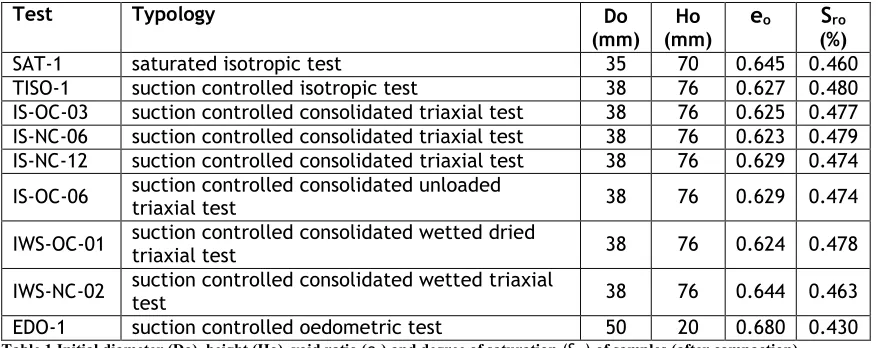
The initial conditions (immediately following compaction) of each of the 9 samples are presented in Table 1 in terms of initial diameter D0 , initial height H0 , initial void ratio e0 and initial degree of saturation Sr0 .

Experimental tests

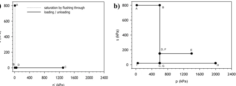
The experimental dataset provided to the participating teams consisted of the results of 9 tests, including two isotropic tests (Figure 2), six triaxial tests (Figure 3) and one oedometer test (Figure 4). For testing of unsaturated samples, control of matric suction was by the axis translation technique.

Test SAT-1 (Figure 2(a)) was an isotropic test involving initial saturation by flushing through (AB in Figure 2(a)) and then isotropic loading (BC) to a mean effective stress of 1300 kPa, followed by isotropic unloading (CD).

Test TISO-1 (Figure 2(b)) was a suction-controlled isotropic test. This involving isotropic loading (AB: s=800kPa, pp 600kPa),wetting/drying (BCD: s 800kPa

 10kPa  150 kPa, p𝑝 = 600kPa), isotropic loading/unloading (DEF: s=150kPa,

pp  600kPa 1400kPa  600 kPa), wetting (FG: s 150kPa  20 kPa, pp =

600kPa), isotropic loading/unloading (GHI: s=20kPa, p𝑝  600kPa  2000kPa 

20 kPa).

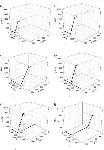
5 of the 6 suction-controlled triaxial tests (Figure 3) involved shearing to failure at a constant suction of 800 kPa, whereas the final triaxial test involved shearing to failure at a suction of 20 kPa.

The stress paths followed in triaxial tests IS-OC-03, IS-NC-06 and IS-NC-12 (Figure 3(a),(b) and (c)) involved “isotropic” loading (AB) at a constant suction of 800 kPa (to a mean net stress of 300, 600 or 1200 kPa respectively) followed by shearing to failure (BCDE) at constant suction and constant radial net stress, with the inclusion of an unload-reload cycle during shearing. A small nominal deviator stress of 10 kPa was applied during “isotropic” stages in all triaxial tests, in order to maintain contact between the loading ram and the sample.

Triaxial tests IS-OC-06 and IWS-OC-01 (Figure 3(d) and (e)) also involved shearing to failure (s = 800kPa; pp = 600kPa) including one or two unload-reload cycles

during shearing. In the former, however, shearing was preceded by “isotropic”

loading/unloading (ABC: s= 800kPa; pp 1600kPa), whereas in the latter, shearing

was preceded by a wetting-drying cycle (BCD: s 800kPa  10kPa  800kPa; p𝑝

= 600kPa). The final triaxial test IWS-NC-02 (Figure 3(f)) involved shearing to failure at a constant suction of 20kPa and a constant radial net stress of 600kPa, following “isotropic” loading (AB: s= 800kPa; pp 600kPa) and then wetting (BC:

s 800kPa  20kPa; pp = 600kPa).

During “isotropic” loading, unloading, wetting or drying stages of all triaxial tests, changes of mean net stress or suction were applied as a series of discrete step changes, each followed by an equalisation period. In contrast, shearing stages (including unloading-reloading) were performed at a constant axial displacement rate of 1.0 μm/min. Participating teams were told to assume that all stages were performed sufficiently slowly to give essentially uniform conditions throughout the sample.

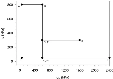
The single suction-controlled oedometer test EDO-1 (Figure 4) involved loading (AB:

v

 = 600kPa), isotropic loading/unloading (DEF: s=300kPa, _v 600kPa 1600kPa

 600kPa), wetting (FG: s  300kPa  50 kPa, _v= 600kPa), isotropic

loading/unloading (GHI: s=50kPa, _v 600kPa  2400kPa  20 kPa). Again each

stage of the oedometer test was applied as a series of discrete step changes of vertical net stress or suction, each followed by an equalisation period.

BENCHMARKING METHODOLOGY

Each team participating in the benchmarking exercise was provided with the same information, consisting of a text with figures describing soil properties, sample preparation and experimental procedures and data sheet file containing the experimental data for the 9 tests. The Excel files contained details of the initial state of each sample immediately following compaction (see Table 1) and the subsequent stress path and stress-strain response for all stages of each test. For isotropic tests, data were provided in terms of mean net stress p , suction s and void ratio e ,

whereas for triaxial tests, data were provided in terms of mean net stress p , deviator

stress q , suction s , void ratio e and axial strain ε1. For the single oedometer test, data

were provided in terms of vertical net stress v , suction s and void ratio e .

Each of the 7 participating teams was required to determine, from the experimental data, values for the 10 BBM soil constants (κ, κs , G , pc , N(0) , λ(0), r , β, M and k )

and an initial value for the hardening parameter p₀(0) . Teams had complete freedom

The overall approach employed by the team from UNINN was very different to the methodology of the other 6 teams. The team from UNINN performed a formal optimization process using inverse analysis. This involved simultaneous optimization of the values of most of the 10 soil constants and the initial value of the hardening parameter, by attempting to minimize suitable objective functions describing the differences between model simulations and experimental results. Exceptions were G ,

M and k , which were determined by the UNINN team in a more conventional fashion.

Each of the 7 teams submitted a return form with their selected values for the 10 BBM soil constants and the initial value of the hardening parameter, together with short descriptions of the procedures that had been employed in estimating these values. The coordinating team from GU compared the 7 parameter value sets, analysed the reasons behind significant differences in proposed parameter values and investigated the implications of these differences. This included performing simulations of all 9 experimental tests with the 7 different sets of parameter values, as well as simulating various fictitious stress paths and investigating other aspects of predicted behaviour.

RESULTS: PARAMETER VALUES

The parameters listed in Table 2 can be divided into five groups: BBM constants describing elastic behaviour (κ, κs and G ); BBM constants giving the variation of λ(s) with suction (λ(0) , r and ); other BBM constants involved in describing yielding

and plastic behaviour under isotropic stress states (pc _{and N(0) ); BBM constants} related to soil strength ( M and k ); and the initial value of the hardening parameter

) 0 ( 0

p . Each of these groups is considered in turn.

Elastic parametersκ, κsand G

The elastic parameters κ, κs and G are generally of relatively minor importance, because elastic strains are typically significantly smaller than plastic strains. Indirect effects of these parameters in the BBM are also normally relatively minor. For example, the value of κ affects the shape of the LC yield curve (through Equation (6)) and the value of κs affects the positions of the normal compression lines for different values of suction (through Equation (4)), and hence the values of these two elastic parameters have some influence on the predicted occurrence and magnitude respectively of collapse compression on wetting, but both of these effects are relatively small.

Table 2 shows that all teams suggested relatively low values for the elastic parameter

κs , consistent with only small magnitudes of elastic swelling or shrinkage induced by suction changes over the experimental range of zero to 800 kPa. However, the values proposed for κs by the different teams varied by almost an order of magnitude, from 0.0005 to 0.0045 . The experimental data used by teams (with the exception of UNINN) in this determination were from wetting or drying stages considered to be inside the LC yield curve. This potentially covered drying stage CD and wetting stage FG from Test TISO-1 (see Figure 2(b)) and drying stage CD from Test IWS-OC-01 (see Figure 3(e)). The results from TISO-1 covered a much smaller range of suction than those from IWS-OC-01, but they were better defined by a number of intermediate points (whereas there were only two data points, at the start and end of drying, for stage CD of Test IWS-OC-01). As a consequence, different teams made different choices of how much weight to give to the results from the two tests in the determination of a value for κs. Inspection showed that there was significant correlation between the emphasis given to the different experimental tests and the value of κs determined, with those teams relying exclusively on the results from TISO-1 generally suggesting lower values for κs than those who also made use of the results from IWS –OC-01.

Inspection of Table 2 shows that the values of shear modulus G determined by the 7 teams varied from 80 MPa to 200 MPa (but with 5 of the 7 values clustered within a range from 120 MPa to 167 MPa). All teams determined the value of G from the unload-reload stages of the triaxial tests. Differences in the proposed value of G were attributable simply to the details of how the experimental unload-reload stress-strain curves were interpreted e.g. the starting and finishing points used when determining the best-fit straight line to the data, whether unload and reload curves were fitted separately or a single line was fitted to an entire unload-reload loop, and whether stress or strain was used as the dependent variable in a least-squares fitting process.

Plastic compressibility parametersλ(0), r and β

The three BBM constants λ(0) , r and β control the variation of plastic compressibility

compression lines at different values of suction (Equation 3). However, by determining the gradients of the lines, they also control the spacing between the normal compression lines for different values of suction at all values of mean net stress other than the reference pressure pc _{(see Equation 3) i.e. they (together with p}c₎ control the spacing between the normal compression lines over the range of p for

which the model will be applied. This means that the three parameters will have an important influence on the predicted magnitude of potential wetting-induced collapse compression and how this varies with p. The three parameters also control (together

with pc _{and, to a lesser degree, κ) the shape of the LC yield curve and how this} develops as it expands (see Equation 6) and hence whether collapse compression will occur during a given wetting path.

Most teams (UNINN was the exception) determined values for λ(0) ,β and r

predominantly by considering the gradients λ(s) of normal compression lines at different values of suction. Several of these teams, however, also took some account of one or more other aspect of behaviour (e.g. the initial shape of the LC yield curve or the spacing between the different normal compression lines).

experimental values, and this was the most important factor behind the different values of λ(0) ,β and r determined by the various teams.

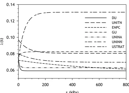
Values of λ(0) , β and r determined by the different teams are given in Table 2 and the corresponding variations of λ(s) with suction predicted by the teams are shown in Figure 5.

Inspection of Figure 5 shows that values of λ(s) predicted by UNINN at suctions above about 50kPa are substantially higher than those predicted by all other teams. In addition, comparison of these predicted values with those determined by fitting data from compression stages in normally consolidated conditions shows that such high values of λ(s) are unrealistic. This indicates the likelihood that the formal optimization process employed by UNINN (involving simultaneous optimisation of multiple parameters) was not successful in identifying a global minimum for the objective function, but instead converged on an inappropriate local minimum. This shows the potential risks of such formal optimisation procedures and emphasises that they should be used only with great caution.

Inspection of Table 2 and Figure 5 shows that the values of λ(0) determined by the different teams varied from 0.072 to 0.097. DU, ENPC and UNINA proposed values between 0.072 and 0.074, based exclusively on the gradient measured in the saturated isotropic test SAT-1. GU and USTRAT proposed slightly higher values (0.078 and 0.080), as a consequence of using additional information in the determination of λ(0). GU determined values for λ(0) and r together, by best-fitting Equation 5 to all experimental values of λ(s) (having previously determined a value for  by another

Inspection of Table 2 shows that all teams except UNINN proposed a value for r close to 1 and hence simulated relatively little variation of λ(s) over the full range of suction (see Figure 5). In contrast, the value proposed by UNINN (r = 1.814) results in much larger variation of λ(s), including unrealistically large values of λ(s) at suctions above about 50kPa, as discussed previously. Of the other teams, GU proposed a value for r

determining a value for β. ENPC assumed as a first tentative estimate a relatively

large value of β (0.1 kPa-1_{), on the assumption of almost constant} 0

p values for s >

800 kPa adjusting it afterword to impose the passage of the LC curve through

determined p0 at s=0 and 800 kPa. This constraint on the LC curve was maintained

while tuning the values of r, β and pc _{to optimize the simulation of the observed} collapse in test TISO-1. In contrast, GU did not consider experimental values of λ(s) at all in determining a value for β , and their procedure was based entirely on attempting to fit the relative spacings between the normal compression lines at different values of suction, because they had identified that this important aspect of behaviour is almost solely dependent on the value of β (see below). The GU procedure for selecting the value of β from the relative spacings of the normal compression lines at different values of suction is set out in Gallipoli, D’Onza and Wheeler (2010).

Parameters pc _{and N(0)}

With the variation of λ(s) with suction defined by the values of λ(0) , r and β and with the value of the elastic parameter κs already determined, the parameters pc and N(0) complete the definition of the normal compression lines for different values of suction (see Equations 3 and 4), by fixing the position of each line. In addition, the value of pc (along with the parameters determining λ(s) and the elastic parameter κ) defines the shape of the LC yield curve and how this develops as it expands (see Equation 6).

Values of pc _{and N(0) determined by the different teams are listed in Table 2. It is not} helpful to compare these values in isolation. For example, the value of pc _{depends on} the value already selected for the parameter r , with pc _{extremely sensitive to r when} the value of r is close to 1. As teams selected different values for r , and many of these are close to 1, widely different values of pc _{have been proposed. For values of r} less than 1, a very low value of pc _{is required (much lower than the range of p over}

which the model is to be applied). Conversely, for values of r greater than 1, a very high value of pc _{is required. In both cases, the required value of p}c _{becomes more} extreme as r approaches 1 (e.g. GU). The required value of N(0) then depends upon the value of pc _{selected, because the intercept N(s) of each normal compression line is} defined at the reference pressure pc _{(see Equations 3 and 4). Hence, given the widely} different values of pc _{selected by the different teams, significant variation in the} values of N(0) is only to be expected.

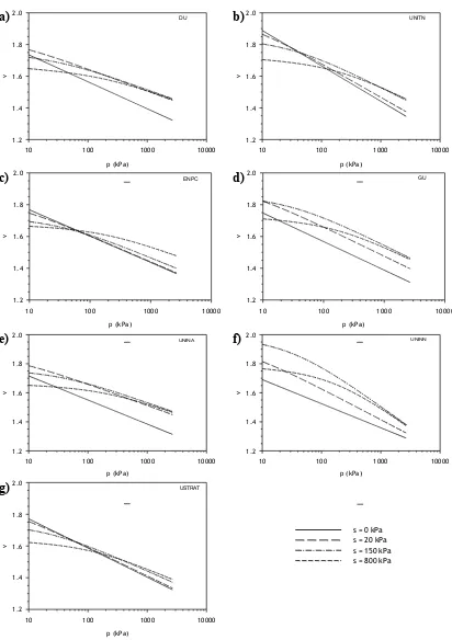
Predicted normal compression lines

Figure 6 shows the resulting normal compression lines predicted by the various teams at s = 0 , s = 20 kPa , s = 150 kPa and s = 800 kPa. There are significant differences between the predictions of the different teams. This is very important, because these normal compression lines give both the magnitude of compression during isotropic loading at constant suction to virgin states and also the variation of potential wetting-induced collapse compression. Hence, the variation between the predictions of the different teams shown in Figure 6 is worrying.

Inspection of Figure 6a-g shows that UNINN predicted normal compression lines that converge significantly as p increases (because their value for r is much greater than

The predicted spacing between the normal compression line at s800kPa and the saturated normal compression line at s0 in Figure 6 is, in almost all cases, essentially dependent on the values of only r and pc _{, because the predicted variation} of λ(s) with suction has essentially stopped by s = 800 kPa (see Figure 5) and any dependency on the value of κs (through Equation 4) is very minor. An exception is ENPC, where the value of  also plays a part, because their very low value of β

means that they predict λ(s) still varying with s for suctions above 800kPa (see Figure 5). Inspection of Figure 6g shows that the spacing between normal compression lines predicted by USTRAT is substantially smaller than that predicted by all other teams. Comparison of normal compression lines predicted by USTRAT with those determined by fitting data from compression stages in normally consolidated conditions shows that the spacing between the s = 800 kPa and s = 0 lines predicted by USTRAT is unrealistically small. This is because a much smaller value of pc should have been used with their value of r (compare with the more realistic spacing of UNINA, figure 6e, who had a similar value of r but a much lower value of pc _{, see} Table 2). The same problem is apparent, to a lesser degree, for some other teams (e.g. UNITN, figure 6b). Conversely, the spacing between the s = 800 kPa and s = 0 lines predicted by UNINN (figure 6f) over most of the range of p of interest is

unrealistically large, because a less extreme value of pc _{should have been used with} their very high vale of r . Note that GU required a very extreme value for pc _{in order} to predict a realistic spacing between the s = 800 kPa and s = 0 lines (figure 6d), because they had a value of r closer to 1 than any other team (see Table 2).

The relative spacing of the normal compression lines for different values of suction in Figure 6 (i.e. where the lines for s = 20 kPa and s = 150 kPa fit between the lines for s

= 800 kPa and s0) depends almost solely on the value of β (the elastic parameter

κs also plays a role, through Equation 4, but this is very minor). DU and UNINA proposed relatively high values of β, and this means that, as shown in Figures 6a,e the

s = 150 kPa line is indistinguishable from the s = 800 kPa line and even the s = 20 kPa line is much closer to the s = 800 kPa line than to the s = 0 line. Conversely, ENPC proposed a low value of β , and this means that the s = 20 kPa line is indistinguishable from the s = 0 line and even the s = 150 kPa line is much closer to the s = 0 line than to the s = 800 kPa line (figure 6c). Other teams employed intermediate values of β . This included GU (figure 6d), who specifically used the experimental evidence on the relative spacing of the normal compression lines at different values of suction in determining a value for β.

Given the crucial importance of accurately capturing the spacing between normal compression lines for different values of suction, and the failure to achieve this by some teams (see Figure 6), the discussion above indicates that it will generally be best to determine a value for β by a method that places the main emphasis on matching the experimental relative spacing between normal compression lines for different values of suction (rather than on attempting to match the experimental variation of λ(s)). This is particularly important when the experimental values of λ(s) cannot be well-matched by BBM (e.g. because they do not vary monotonically with suction), and hence differences of procedural detail may lead to widely different values of β if the methodology is based on attempting to match the experimental variation of λ(s)).

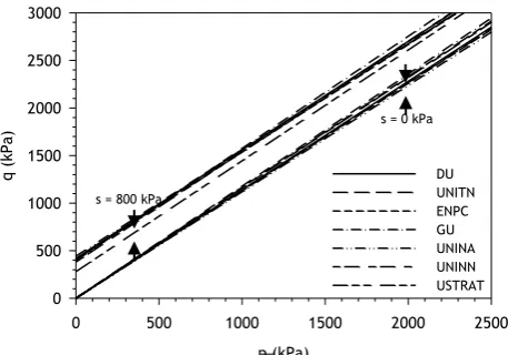
Strength parameters M and k and predicted critical state lines

Parameters M and k determine the positions in the q:p plane of critical state lines for

different values of suction (see Equation 10). Each of the six triaxial tests involved constant suction shearing to a critical state (five at s = 800 kPa and one at s = 20 kPa), and all teams used the experimental critical state values of q and p from these tests to

consequence, the values of M and k proposed by the various teams are all very consistent (see Table 2), with M in the range 1.12 to 1.18 and k generally in the range 0.41 to 0.50. The locations of the critical state lines in the q:p plane predicted by the

various teams are therefore very similar (see Figure 7). A minor discrepancy is that USTRAT proposed a significantly lower value of k (k = 0.3) than other teams, resulting in the prediction of lower critical state values of q than other teams at suctions greater than zero (see Figure 7).

Figure 8 shows the critical state lines in the v:ln p plane predicted by the various

teams (from Equation 11). As indicated by Equation 11, each critical state line is curved in the v:ln p plane, with the exception of the saturated line at s0. Inspection

of Figure 8 shows large differences between the predictions of the different teams. This is mainly attributable to differences in the predictions for the corresponding normal compression lines (see Figure 6). Comparison of Equation 11 with Equation 3 shows that the predicted spacing v between the critical state line for a given value of suction and the corresponding normal compression line varies with p and is given

by:

 





  

 

 

 

p ks s

v   ln 2 (12)

Teams generally proposed reasonably similar values of κ and k , and most teams (with the exception of UNINN) predict reasonably similar values of λ(s) (see Figure 5). Hence, from Equation 12, the different teams predict reasonably similar variation with s and p of the spacing between each critical state line and the corresponding normal

compression line. This means that (with the exception of UNINN) teams predict reasonably similar reductions of v during constant suction shearing of a normally consolidated soil from the normal compression line to the critical state line (see later).

Initial value of p₀

 

The initial value of the hardening parameter p₀

 

LC yield surface in BBM. The initial shape of the LC yield curve in the s:p plane is

the variation of λ(s) with suction (λ(0) , r and β). Experimental values of yield stress under isotropic stress states (showing the initial form of the LC yield curve, and hence

useful to the teams in determination of an initial value for p₀

 

= 0 (SAT-1) and s = 800 kPa (IS-NC-12 and IS-OC-06).

Table 2 shows that the initial values of p0

 

from 42 kPa to 291 kPa. The formal optimisation procedure employed by UNINN resulted in a lower value (42 kPa) than those determined by all other teams, and again comparison with the experimental results suggests that the procedure had failed to identify a true set of optimum parameter values. DU, GU and UNINA based their

initial values of p₀

 

in the saturated test (SAT-1) and hence they all suggested similar values for p₀

 

kPa to 85 kPa). As stated earlier, UNITN were unhappy about the consistency of the experimental results from SAT-1 and they therefore back-calculated their initial value

of p0

 

IS-OC-06), leading to a much higher initial value for p₀

 

either took account of experimental yield points at both s = 0 and s = 800 kPa or attempted to best match patterns of collapse compression in Test TISO-1, and these

approaches resulted in intermediate initial values of p0

 

Figure 9 shows the initial forms of the LC yield curve predicted by the different teams, with Figure 9(a) showing the predicted curves over the full experimental range of suction whereas Figure 9(b) shows an expanded view of the curves for low values of suction (up to s = 100 kPa). There are very significant differences between the forms of curve predicted by the various teams. These reflect the differences in the forms of normal compression lines predicted by the different teams (see Figure 6), because once the normal compression lines for different values of suction are defined (together with the values of the elastic parameters κ and κs ) this fixes the form of the LC yield curve and how it develops during expansion.

Inspection of Figure 9(b) shows that the predicted yield stress at s = 0 varies from 42

selected by the different teams. Inspection of Figure 9(b) shows that the predicted yield stress as suction tends to infinity varies from 193 kPa (USTRAT) to 1011 kPa (UNINN) and 1563 kPa (ENPC) (this limiting value predicted by ENPC is only approached at suctions considerably greater than the range shown in the figure). Consideration of the LC yield curve expression of Equation 6 shows that the predicted

ratio of the yield stress at s =  to the yield stress at s = 0 , p₀

   

function mainly of the values of _p

 

0 and r (with a small influence of the value of κ/λ(0) ). The predicted ratio p₀

   

proposed value of pc _{is relatively extreme for their value of r (which is much greater}

than 1). In contrast, the ratio p0

   

proposed value of pc _{is insufficiently extreme for their value of r (which is relatively} close to 1).

Figure 9(a) illustrates that selection of a low value for β (e.g. ENPC) results in a yield

curve shape where the yield stress p0 continues to vary significantly over a wide

range of suctions. In contrast, selection of a high value for β (e.g. DU or UNINA)

results in a yield curve shape where all significant variation of p₀ occurs for suctions

less than about 50 kPa.

RESULTS: SIMULATIONS OF SELECTED TESTS

Saturated isotropic test SAT-1

Figure 10(a) shows the stress path for the saturated isotropic test SAT-1. Figure 10(b) shows the experimental results (in the v : ln p' plane) from the isotropic loading and unloading stages BCD, together with the corresponding model simulations using the 7 different parameter value sets.

Inspection of Figure 10(b) shows that all 7 teams predicted reasonably similar gradients for the saturated isotropic normal compression line (λ(0)) and for the pre-yield compression curve during loading and the swelling curve during unloading (κ) and that these all provided reasonable matches to the corresponding experimental gradients. There were however significant variations in the predictions of the yield stress during loading and the location of the saturated normal compression line, and in some cases the match to the experimental results was relatively poor.

The yield stress and the location of the saturated normal compression line in Test SAT-1 were well-matched by DU, GU and UNINA, as a consequence of the fact that these features were explicitly fitted in the parameter value selection procedures used by these teams. In contrast, the UNITN team explicitly ignored the results from Test SAT-1, because they considered them to be inconsistent with the results from the remaining tests, and as a consequence Figure 10(b) shows that they significantly overestimated the yield stress observed in this test and predicted that the saturated isotropic normal compression line was significantly above its observed position. This mis-match was linked to the fact that UNITN predicted the saturated isotropic normal compression line to be very close to the normal compression line for s = 20 kPa (see Figure 6(b)). The teams from ENPC and USTRAT also predicted that the saturated isotropic normal compression line was very close to the normal compression line for s

they underestimated the yield stress in Test SAT-1 and predicted that the saturated isotropic normal compression line was below its observed position (see Figure 10(b)).

Isotropic test TISO-1

Figure 11(a) shows the stress path for the suction-controlled isotropic test TISO-1. Figures 11(b) to 11(h) show the experimental results (in the v: lnp plane) for all test

stages and the corresponding 7 different model simulations. The experimental results appear to show elastic behaviour during initial loading stage AB, significant collapse compression during wetting stage BC, very small (elastic) shrinkage and swelling during drying stage CD and wetting stage FG respectively, yielding and plastic compression during loading stages DE and GH and elastic swelling during unloading stages EF and HI. All of this behaviour is qualitatively consistent with BBM, in the sense of very small (elastic) shrinkage/swelling while the stress point moves inside the LC yield locus either during loading/unloading or drying/wettingand significant compression during wetting and loading stages where yielding on the LC yield locus is expected.

Inspection of Figure 11(b) and Figure 11(h) shows that DU and USTRAT incorrectly predict that yielding would occur during the initial loading at a suction of 800 kPa (stage AB). This is attributable to the fact that the initial shape of the LC yield curve predicted by these two teams (USTRAT in particular) involves low values of yield stress at high suctions (see Figure 9(a)). In addition, DU under-predicts the magnitude of collapse compression during wetting stage BC and hence the final volumetric strain at the end of the test, as a consequence of under-predicting the spacing between the normal compression lines for s = 800 kPa and s = 20 kPa (largely due to the relatively high value of β proposed by DU). In contrast, USTRAT over-predicts the final volumetric strain at the end of the test, because the locations of the normal compression lines for all four experimental values of suction are poorly predicted.

Inspection of Figure 11(c) and Figure 11(e) shows that both UNITN and GU provide good matches to the magnitude of collapse compression during wetting stage BC and to the final volumetric strain at the end of the test, largely as a consequence of predicting an appropriate spacing between the normal compression lines for s = 800 kPa and s = 20 kPa (see Figure 6). However, both UNITN and GU incorrectly predict little or no plastic straining during loading stage DE at an intermediate suction of 150 kPa. This is because these two teams did not match well the experimental position of the normal compression line at s = 150 kPa. This illustrates the fact that with BBM it was impossible to match well the observed positions of the normal compression lines for all 4 experimental values of suction (s = 0 from Test SAT-1, s = 20 kPa and s = 150 kPa from Test TISO-1 and s = 800 kPa from triaxial tests IS-NC-12 and IS-OC-06). This was because the experimental results indicated large spacing between the s = 0 and s = 20 kPa lines, small spacing between the s = 20 kPa and s = 150 kPa lines, but then large spacing again between the s = 150 kPa and s = 800 kPa lines, and this type of irregular spacing could not be captured by BBM. Therefore, even if matching the positions of the normal compression lines was given over-riding priority in the parameter value selection procedure, it was at best only possible to match three of the four experimentally observed locations of normal compression lines. For example, GU placed great emphasis on matching normal compression line locations, but they explicitly chose to match well the normal compression lines for s = 0, s = 20 kPa and

Inspection of Figure 11(g) shows that UNINN was another team who incorrectly predicted no plastic straining during loading stage DE at the intermediate suction of 150 kPa, but they also over-predicted both the magnitude of collapse compression during wetting stage BC and the final volumetric strain at the end of the test. This was a consequence of their formal optimisation procedure resulting in poor matching of the positions of normal compression lines for most values of suction.

Triaxial test IS-NC-12

Figure 12(a) shows the stress path for suction-controlled triaxial test IS-NC-12. Experimental data (dotted line highlighted by solid triangles) of initial isotropic loading stage AB (at a suction of 800 kPa) are shown in Figure 12(b) (in the v: lnp

plane), together with the corresponding model simulations using the 7 parameter value sets. UNITN, ENPC, GU, UNINA and UNINN all provide satisfactory matching of the experimental results during initial isotropic loading, whereas DU and particularly USTRAT underestimate the yield stress and predict that the normal compression line for s = 800 kPa is below the observed position. This is attributable to the fact that the initial shape of the LC yield curve predicted by these two teams involves low values of yield stress at high suctions (see Figure 9(a)).

Figure 12(c) and Figure 12(d) show the experimental data (dotted lines) and model predictions for the shearing stage BCDE, as plots of deviator stress q against axial strain ε1 and volumetric strain εv against shear strain εs . The unload-reload loop has been omitted from the model predictions for clarity.

Inspection of Figure 12(c) shows that all teams predicted very similar values of final critical state deviator stress, as a consequence of selecting very similar values for the strength parameters M and k . These predictions of final critical state deviator stress are all good matches to the experimental result.

overestimate the compression observed in the experiment (DU provides the closest match). The reason that most of the teams predict similar magnitudes of compression during this drained shearing of a normally consolidated soil is that they predict very similar spacing between the normal compression line and the critical state line in the

v: lnp plane (see Equation 12). The exception is UNINN, who predict a much larger

magnitude of compression than other teams during this shearing stage (see Figure 12(d)), because they have a much larger spacing between normal compression line and critical state line at a suction of 800 kPa than other teams, because they predict a much higher value of λ(s) at s = 800 kPa than other teams (see Figure 5) and this has a crucial influence on Equation 12.

Returning to Figure 12(c), it can be seen that most teams significantly under-predict the development of axial strain at values of deviator stress less than the final critical state value, indicating that shear strains are under-predicted. Given that volumetric strains are somewhat over-predicted (see Figure 12(d)), the under-prediction of shear strains means that the flow rule of Equation 9 is not providing a good match to the experimental behaviour. This indicates a weakness of BBM, rather than a weakness of the parameter value selection procedures employed by the various teams. It should be noted that the form of the flow rule given by Equation 9, including the expression for

α, was proposed by Alonso, Gens and Josa (1990) to match empirical experience of the value of K0 for normally consolidated saturated soils, but this does not guarantee that Equation 9 matches observed behaviour when a soil is unsaturated or when the stress ratio corresponds to conditions other than one-dimensional straining. Inspection of Figure 12(c) shows that UNINN provides a better match than other teams to the experimentally observed development of axial strains prior to failure. This is, however, a consequence of two counter-acting errors: they substantially over-predict the volumetric strains (see Figure 12(d)) and when the inaccurate flow rule of Equation 12 is then applied to these volumetric strains this fortuitously results in prediction of shear strains which show a good match to the experimental results.

Figure 13(a) presents the stress path for suction-controlled triaxial test IWS-OC-01, showing a wetting-drying cycle BCD (down to a suction of 10 kPa) prior to final shearing at a suction of 800 kPa. This represents shearing of an overconsolidated sample, where the overconsolidation has been produced by the previous wetting-drying cycle (the wetting leads to expansion of the yield surface). Experimental results from the shearing stage DEFGHI are shown (dotted lines) in Figure 13(b) (in the q : ε1 plane) and Figure 13(c) (in the εv : εs plane), together with the corresponding model predictions. The two unload-reload loops have been omitted from the model predictions for clarity. Experimental data show a dilation (Figure 13(c)) non occurring in conjunction with a peak of deviator stress (Figure 13(b)). This kind of behaviour can't be predicted by the model, regardless of parameters values.

Figure 13(a) and Figure 13(b) show that the model simulations divide into two groups. DU, UNITN, UNINA and USTRAT predict yielding on the wet side of critical state for this overconsolidated sample, and hence they predict no occurrence of a peak deviator stress prior to reaching a critical state (Figure 13(b)) and positive volumetric strain (compression) during shearing (Figure 13(c)). In contrast, ENPC, GU and UNINN predict yielding on the dry side of critical state, and hence they predict a peak deviator stress and then post-peak softening to a critical state (Figure 13(b)) as well as negative volumetric strain (dilation) during shearing (Figure 13(c)). This difference is caused by the fact that the expanded shape of the LC yield surface after wetting to s = 10 kPa (with p = 600 kPa) varies significantly between the

different teams. In particular, ENPC, GU and UNINN predict that, after wetting-induced expansion, the cross-section of the yield surface at s = 800 kPa is considerably larger than predicted by the other 4 teams. Inspection of Figure 13(b) shows that the q : ε1 simulations of those teams who predict yielding on the wet side of critical state are much closer to the experimentally observed behaviour than those of the teams who predict yielding on the dry side. In terms of volumetric strains (Figure 13(c)), the experimental results show initial compression during shearing and then dilation, with the magnitude of final dilation being substantially greater than predicted by even the 3 teams who show yielding on the dry side.

Figure 14(a) shows the stress path for the suction-controlled oedometer test EDO-1 in

a plot of suction against vertical net stress _v . The experimental stress path in the q :

p plane is unknown, because there were no experimental measurements of horizontal

stress.

The variation of horizontal net stress in an oedometer test is determined by the zero lateral strain condition and is therefore influenced by the material behaviour. As a consequence, each of the 7 different model simulations of oedometer test EDO-1 (each with a different parameter value set) shows a different predicted variation of horizontal net stress and hence a different stress path in the q:p plane. Figure 14(b)

shows the predicted stress path in the q:p plane using the parameter value set

proposed by ENPC. The stress paths predicted by other teams showed significantly different values of stress, but common qualitative features.

Inspection of Figure 14(b) shows that each of the loading stages AB, DE and GH involves an initial elastic section of stress path and then a yield point followed by an elasto-plastic section of stress path. The gradient of the elastic sections varies with p

(and, to a lesser extent, specific volume v ), because of the assumption of a constant elastic shear modulus G (Equation 2) in combination with a variable elastic bulk modulus K (through Equation 1). For example, the initial elastic section of stress path AB has a very steep gradient in the q:p plot, whereas the initial elastic section of

stress path GH has a much shallower gradient (see Figure 14(b)). The subsequent elasto-plastic sections of the stress paths for loading stages AB, DE and GH each initially traverses around the yield curve (with only modest expansion of the curve),

until the stress ratio q





The stress paths for unloading stages EF and HI in Figure 14(b) are both entirely elastic. Finally, the stress paths for wetting stages BC and FG and drying stage CD all

have a gradient of 3 2 in the q:p plane (see Figure 14(b)), simply as a

consequence of the fact that vertical net stress _v was constant during these stages.

Figure 15 shows the experimental results of oedometer test EDO-1 in the v : lnv

plane, together with the 7 different model predictions. Features of the experimental results in Figure 15 include collapse compression during wetting stage BC and elasto-plastic compression during loading stages DE and GH. Almost all the teams made no use of the oedometer test results in their parameter value selection procedures, because the predicted stress path for the oedometer test was both highly complex and also impossible to specify precisely until the model parameter values were selected.

The model simulations in Figure 15 predict the qualitative behaviour with varying degrees of success, but all model simulations show significant errors in the magnitude of predicted volumetric strain during at least one stage, and the final volumetric strain by the end of the test is poorly predicted by most teams. The model predictions for the oedometer test generally show significantly poorer matches with the experimental results than those for the isotropic tests and triaxial tests. This can be partly attributed to the fact that the oedometer test results were not used in the process of determining parameter values. An additional factor, however, is that the predicted response during suction-controlled oedometer tests is even more sensitive to the material behaviour than that during isotropic or triaxial tests, because even the stress path followed is strongly influenced by the material behaviour.

RESULTS: OTHER IMPLICATIONS

during application of BBM in numerical modelling of a boundary value problem). This issue was explored by the coordinating team from GU, who simulated various fictitious stress paths with the 7 different parameter value sets and also investigated other aspects of predicted behaviour. Two of these aspects are presented here for illustration.

Predicted development of LC yield curve shape during expansion

Figure 9 already demonstrated that the parameter value sets proposed by the 7 teams resulted in very significant differences in the predictions of initial shape and position of the LC yield curve. Figure 16 illustrates how these differences in yield curve shape develop as the LC yield curve expands. Figure 16(a) shows the LC yield curve shape predicted by each of the 7 teams when a common value of saturated isotropic yield

stress p0

 

average initial value of p₀

 

development of LC yield curve shape after expansion to p0

 

The shape of the LC yield curve determines, amongst other things, whether collapse compression will occur during a given wetting path and the value of suction at which this collapse compression will commence. Figures 16(a) and 16(b) show that the 7 different parameter value sets proposed by the 7 teams will inevitably lead to very different predictions of volume change during wetting, and that these differences will remain large even after expansion of the LC yield curve.

Closer inspection of Figures 16(a) and 16(b) also shows that the relative positions of the LC yield curve predicted by the different teams can change during expansion. For example, in Figure 16(a) the yield stress predicted at a suction of 800 kPa is largest for UNINN, followed by GU, UNINA and DU in sequence, whereas in Figure 16(b) the order has changed to UNINA followed by GU, DU and UNINN in sequence. Further changes of order occur as the yield curve is expanded to even higher values of

 

p . This indicates that, amongst other things, differences in predicted behaviour

Predicted behaviour during wetting

Differences in predicted behaviour during wetting are explored further in Figure 17. This figure shows the predicted variation of specific volume v during wetting paths from s = 800 kPa to s = 0 under an isotropic stress state conducted at p= 100 kPa

(Figure 17(a)), p= 200 kPa (Figure 17(b)) or p= 500 kPa (Figure 17(c)). Each part

of the figure should be read from right to left, as suction is reduced during a wetting path. The predictions shown in Figure 17 are for the 7 different parameter value sets,

including the 7 different initial values of p0

 

consisting of simple isotropic loading at s = 800 kPa to the start of the wetting path.

In Figure 17(a) all predictions show elastic swelling through the majority of the wetting path, because the initial stress state at p=100 kPa , s = 800 kPa is inside the

initial location of the LC yield curve in all cases (see Figure 9(a)). UNITN, ENPC and USTRAT predict that swelling continues throughout the entire wetting path, with the wetting path remaining inside the LC yield curve (see Figure 9(b)), because these 3

teams proposed initial values of p₀

 

close inspection of Figure 17(a) shows that the other 4 teams predict varying amounts of collapse compression in the very last part of the wetting path as the LC yield curve

is reached (see Figure 9(b)), because these 4 teams proposed initial values of p0

 

less than 100 kPa (see Table 2).

In Figure 17(b), where the wetting takes place at p= 200 kPa , UNINN is now the

only team that predicts swelling throughout the entire wetting path, because they are

the only team that proposed an initial value of p₀

 

and hence they are the only team to predict that the LC yield curve is not reached during wetting. At the opposite extreme, USTRAT predicts that the stress state will be already on the LC yield curve at the start of wetting, because they predict an initial

location of the yield curve with a yield stress p0 less than 200 kPa when the suction is

less than the magnitude of negative elastic volumetric strain (elastic swelling) and hence the collapse compression is hidden and a net swelling response is predicted (see Figure 17(b)). The small magnitude of positive plastic volumetric strains predicted during the early part of wetting is a consequence of the very steep gradient of the LC yield curve at these higher values of suction (see Figure 9(a)). As the suction is reduced (and the LC yield curve becomes less steep), USTRAT predicts that the magnitude of plastic volumetric strain increments gradually increases and the overall response gradually changes from swelling to collapse compression, with no sudden change of behaviour (see Figure 17(b)). In contrast, ENPC, UNINN, GU, UNINA and DU predict that, when the wetting takes place at p= 200 kPa, the LC yield curve will

be reached late in the wetting process (see Figure 9), when the LC yield curve is not very steep, and hence a sudden change from swelling (elastic behaviour) to collapse compression (plastic behaviour) is predicted late in the wetting path (see Figure 17(b)).

Figure 17(c) shows that when wetting takes place at p= 500 kPa all teams predict