Classification of Hyperspectral Images by Exploiting
Spectral-Spatial Information of Superpixel via Multiple
Kernels
Leyuan Fang, Member, IEEE, Shutao Li, SeniorMember, IEEE,Wuhui Duan,
Jinchang Ren, andJón Atli Benediktsson, Fellow, IEEE
Abstract—For the classification of hyperspectral images (HSIs), this paper
presents a novel framework to effectively utilize the spectral-spatial information of superpixels via multiple kernels, termed as superpixel-based classification via multiple kernels (SC-MK). In HSI, each superpixel can be regarded as a shape-adaptive region which consists of a number of spatial-neighboring pixels with very similar spectral characteristics. Firstly, the proposed SC-MK method adopts an over-segmentation algorithm to cluster the HSI into many superpixels. Then, three kernels are separately employed for the utilization of the spectral information as well as spatial information within and among superpixels. Finally, the three kernels are combined together and incorporated into a support vector machines classifier. Experimental results on three widely used real HSIs indicate that the proposed SC-MK approach outperforms several well-known classification methods.
Index Terms—Hyperspectral image, Superpixel, Multiple kernels, Spectral-spatial image classification, Support Vector Machines.
I. INTRODUCTION
Hyperspectral imaging has been widely used in the remote sensing which can acquire
images from hundreds of narrow contiguous bands, spanning the visible-to-infrared
spectrum. In the hyperspectral image (HSI), each pixel is a high-dimensional vector
and its entries represent the spectral responses of different spectral bands. The highly
This work was supported in part by the National Natural Science Foundation of China under Grant No. 61172161, the National Natural Science Foundation for Distinguished Young Scholars of China under Grant No. 61325007, and the Fundamental Research Funds for the Central Universities, Hunan University.
L. Fang, S. Li, and W. Duan are with the College of Electrical and Information Engineering, Hunan University, Changsha, 410082, China (email: [email protected] [email protected]; [email protected]).
J. Ren is with the Centre for excellence in Signal and Image Processing, Department of Electronic and Electrical Engineering, University of Strathclyde, Glasgow, U.K. (email: [email protected])
informative spectral information of the HSI pixels has many applications, such as
classification [1], target detection [2], anomaly detection [3], spectral unmixing [4],
and others [5].
In the last decades, HSI classification has been a very active research topic in the
remote sensing. Given a representative training set for each class, the objective of the
classification is to assign each pixel to one of the classes based on its spectral
characteristics. To achieve this, many discriminative approaches have been developed.
Among these, the support vector machine (SVM) [6, 7] and multinomial logistic
regression (MLR) [8-10] have demonstrated to be very powerful. Dynamic or random
subspace [11, 12], which are new version of random forest and exploit the inherent
subspace structure of hyperspectral, have proved to be an effective way for analyzing
and classifying HSIs. The sparse representation [13-15], which can sparsely
decompose the input pixel on an over-complete dictionary, is another widely used
classifier. Recently, metric learning [16] has also been successfully explored in
hyperspectral image processing, which has formulated a novel and adaptive metric
learning method for classification and object recognition. In addition, some other
classification approaches have focused on the design of effective feature extraction or
reduction techniques, such as the principle component analysis [17], clonal selection
feature-selection [18], kernel discriminative analysis [19], and semisupervised
discriminative locally enhanced alignment [20]. Note that, kernel [21] has been
widely used in the aforementioned approaches, since it can improve the class
Although the above approaches can effectively utilize the spectral information,
their classification results often appear very noisy. This is mainly due to the two facts
that the number of reference training samples is often very limited and the spectral
information of pixels from one class may be easily mixed with that of pixels from
other classes. To further improve the classification performance, some recent works
attempt to use both the spectral information and spatial information of the HSI, which
is based on the assumption that pixels from a local spatial region should have very
similar spectral characteristics and thus correspond to the same materials. In [23, 24],
the extended morphological profiles (EMP) is used to exploit the spatial information,
which can effectively improve the estimation. In [25], the spatial dependence of pixels
within a local region is exploited by a postprocessing procedure on each individual
pixel label. In [13], the spatial information is incorporated into the sparse
representation technique by a joint sparse norm on pixels within a local region. In [26],
multiple kernels are utilized for the exploration of the spatial information, which is
modeled as the mean and variance of pixels within a local region. Though the above
works [13, 25, 26] can provide promising classification accuracies, the size and shape
of the adopted spatial region is fixed and thus the spatial context in HSI may not be
sufficiently exploited. That is, the shape of the regions should be changed according
to different spatial structures of the HSI. For example, large region sizes should be
selected for the smooth area while heterogeneous spatial area requires small region
In computer vision field, superpixel has been extensively investigated to facilitate
the visual recognition [27-29]. Each superpixel is a local region, whose size and shape
can be adaptively adjusted according to local structures. In this paper, we introduce
the superpixel for the HSI classification and propose to effectively exploit both the
spectral and spatial information of the superpixel via multiple kernels, which is
denoted as the superpixel-based classification via multiple kernels (SC-MK). Firstly,
the SC-MK adopts an efficient over-segmentation algorithm [29] to cluster the HSI
into many superpixles. Then, mean filtering and weighted average filtering are
utilized to extract the spatial features within and among superpixels. Subsequently,
three kernels are separately computed on the pixels extracted from the original
spectral feature as well as the spatial features within and among superpixels. Finally,
the three kernels are combined together and incorporated into the support vector
machines classifier. Note that, in some very recent works [30, 31], the HSI is also
classified based on the superpixel. These works [30, 31] use histogram descriptors or
K-means clustering for the classification, and do not consider the correlations among
superpixels. In addition, some works have recently applied the multiple kernels for
HSI classification [32, 33]. In [32], the multiple kernels have been incorporated into a
domain adaptation framework to reduce the bias between source and target domains.
The work in [33] employed a learning algorithm to adaptively select multiple
representative kernels for classification. In contrast, the proposed SC-MK method
and among superpixels, which is different from the above superpixel-based and
multiple kernels based works [30-33].
The rest of the paper is organized as follows. In Section II, the support vector
machines with multiple kernels for HSI classification are briefly reviewed. Section III
introduces the proposed SC-MK method. Experimental results on three well-known
HSI data are presented in Section IV. Section V concludes this paper and suggests
future works.
II. SUPPORT VECTOR MACHINES (SVM) WITH MULTIPLE KERNELS
SVM is a supervised learning models and its objective in HSI classification
problem is to find a decision rule which can determine the class label for each test
pixel [6, 7]. Since the real HSI pixel is linearly non-separable, the SVM usually
adopts a kernel function to map pixels into the high-dimensional feature spaces. To be
specific, let
1,...,
M N y y denote the training pixels and
c1,...,cN
represent the corresponding class labels. The SVM aims to solve the following problem:
2
, ,
1
min subject to , 1 , 1,...,
2
0, 1,...,
i
i i i i
b
i
i
T c b i N
i N
w w y w (1)
where
w
and b define the classifier in the feature space,
i are the slack variablesfor the nonseparability of data, and T is a regularization parameter that controls the
generalization ability of the classifier.
is a mapping function, which transforms the input pixel 1 My into a higher dimensional feature space
M* i y
*
i, j
i ,
j .K y y
y
y (2) Then, we can construct a non-linear SVM by the kernel function, without consideringthe mapping
explicitly. The most widely used kernel is the radial basis function(RBF) kernel, which is computed as
2 2
exp
, 2 .
i j i j
K y y y y
(3) Then, by incorporating (2) into (1), we solve a dual Lagrangian problem and obtainthe decision rule for any test pixels:
1
( ) N i i i,
i
K b
f c
y y y (4)
where
i are the Lagrange multipliers in (1), which can be estimated by quadraticprogramming (QP) methods [34].
If the RBF kernel is created from the original spectral pixels
1Spec,..., Spec
Ny y , the
corresponding kernel is denoted as the spectral kernel
Spe ,
Spec
c Spec
i j
K y y . In [26], to
further exploit the spatial information of the HSI, one spatial region (of fixed size) is
defined for each pixel in HSI and the mean or variance is computed for pixels within
each region as the spatial feature. Then, a new RBF kernel can be computed on the
pixels
1Spat,..., at
N Spy y from the spatial feature and it is called as the spatial kernel
Spat, Spat
S atp i j
K y y . Finally, a composite kernel can be effectively computed by a
weighted average of these two kernels:
,
Spec, Sp
Spat, Spat
,CW Spec Spec Spat
ec
i j i j Spat i j
K y y K y y K y y (5)
where Spec and Spat are the weights for the spatial kernel
Spe ,
Spec
c Spec
i j
K y y and
spectral kernel
Spat, Spat
S atp i jK y y , respectively, and SpecSpat 1. The composite
rule for classification. Compared to the single spectral kernel, the composite kernel
considers the spatial information and thus can enhance the HSI classification
performance. However, since the size of the adopted spatial region is fixed, the spatial
information still may not be sufficiently exploited. For example, if the region-size for
the test pixel is selected too large in the detailed region (see blue region in Fig. 1(a)),
some pixels uncorrelated to the test pixel might be included, thus deteriorating the
classification accuracy. In contrast, if the region-size is chosen too small for the pixel
in the smooth region (see green region in Fig. 1(a)), the spatial information cannot be
sufficiently exploited for the classification.
[image:7.595.179.422.350.525.2]
(a) (b)
Fig. 1. Spatial region selection by (a) fixed-size rectangles; and (b) adaptive-size superpixels.
III. SUPERPIXEL BASED CLASSIFICATION VIA MULTIPLE KERNELS (SC-MK)
In computer vision field, the superpixel has been studied for an efficient
representation, which can facilitate visual recognition [27-29]. Each superpixel is a
perceptually meaningful region, whose shape and size can be adaptively changed
according to different spatial structures (see an example in Fig.1(b)) [28]. In this
paper, the proposed SC-MK algorithm extends the superpixel for HSI classification
within and among each superpixel. In general, the proposed SC-MK algorithm
consists of the two parts: a) Creation of superpixels in HSI, and b) Exploration of
spectral-spatial information of superpixel via multiple kernels, which will be
described in the following two subsections.
A. Creation of Superpixels in HSI
Unlike the single-band gray or three-band color image, the HSI usually has
hundreds of spectral bands. To improve the computational efficiency, principle
component analysis (PCA) [35] is firstly used to reduce the spectral bands of the HSI.
Since the important information of the HSI is existed in the principle components
(e.g., first three principle components), they are used as the base images.
Secondly, the superpixel number L is selected based on the complexness of the
structural texture in HSI. Specifically, the Sobel filter [36] which is a simple texture
detector is first applied on the base images. Then, the number of non-zero elements in
the filtered images is compared with the total number of pixels in the base images to
create a texture ratio Rtexture, which reflects the complexness of texture in HSI. Finally,
the superpixel number L is selected by the texture ratio Rtexture and a predefined base
superpixel number Lbase,
base texture.
L L R (6)
Note that, other advanced texture detectors might be used to enhance the performance,
but will create more computational cost.
Thirdly, given the superpixel number L, an over-segmentation algorithm called
entropy rate superpixel (ERS) [29] is applied on the base images to generate a 2-D
superpixel map. Specifically, the ERS is graph-based clustering algorithm, which first
to pixels of the base images and E is the edge set representing the pair-wise
similarities between adjacent pixels. Then, the ERS segments the graph into L
connected subgraphs (each corresponds to a superpixel) by selecting a subset of edges
AE. To form the compact, homogeneous and balanced superpixels, an entropy rate
term H
and a balancing term B
are incorporated into the objective function of the superpixel segmentation:
max H B subject to
A A AE (7)
where 0is the weight for controlling the contribution of the entropy rate term and
balancing term. The problem (7) can be efficiently solved by a greedy algorithm
introduced in [37].
Finally, for the 2-D superpixel map, the position indexes of pixels within each
superpixel can be obtained. Then, the position indexes for L superpixels in the 2-D
map can be applied on the original HSI to extract the corresponding L
non-overlapping 3-D superpixels. The procedure for the creation of the superpixels in
[image:9.595.100.499.504.693.2]HSI is illustrated in Fig. 2.
Fig. 2. The procedure for the creation of superpixels in HSI.
In this subsection, we will first introduce how to utilize the superpixels to create
three feature images which separately reflects the spectral information and spatial
information within and among superpixels. Then, three kernels are computed on the
pixels from the feature images to exploit the spectral-spatial information of
superpixel.
Each superpixel is a group of neighboring spectral pixels z, 1,..., Z
i z
y , which can
be transformed into a matrix SP
i
Y . As described in the Section II, spectral pixels
representing the spectral information of superpixels in HSI can be directly used as the
spectral feature. All the spectral pixels in HSI constitute the spectral feature image
Spec
I .
To exploit the spatial information within each superpixel, a mean operation is first
applied on the spectral pixels [ ,...,1 Z]
i i
y y within each superpixel YiSP and then the
mean pixel Mean i
y is assigned to all pixels in each superpixel. Here, the YiSP is still
the superpixel, which consists of a number of spectral pixels. This operation is the
same as the mean filtering (which is also adopted in the work [38]) and can reduce the
interferences (e.g., noise) in each superpixel. All the filtered superpixels can constitute
a mean feature image Mean
I . Note that, adopting other more powerful filtering
approaches (e.g., Laplacian filtering and guided filtering [39]) might enhance the
Fig. 3. An example showing the current processed superpixel SP
i
Y and its
neighboring superpixels
Y
iSP,1,....,
Y
iSP,8.To exploit the spatial information among superpixels, a weighted average operation
is conducted on the neighboring superpixels Yi jSP, ,j1,...,J of the current processed superpixels YiSP (see an example in Fig. 3), where J is the number of neighboring
superpixels. Since the mean pixel is the representative feature of each superpixel, the
weighted average operation can also be applied on the mean pixels yi jMean, , j1,...,J of neighboring superpixels and a weighted average pixel can be obtained by:
J
WA Mean
, ,
1
i i j i j j
w
y y (8)
where wi j, is the weight, which is estimated as [40],
Mean Mean 2
, 2
,
exp
.
Norm
i j i i j
h
w
y
y
(9)In (9), Norm is defined as
Mean, Mean 22
1exp
J
i j i
j
h
y y and h is a predefinedscalar. Then, the yWAi is assigned to all pixels in each superpixel YiSP and all the
superpixels constitute a weighted average feature image Weigh
I .
In the training stage, firstly, a set of spectral pixels
y1,...,yN
are randomly (ormanually) selected from the original HSI. Then, the position indexes for these
selected pixels are used to extract pixels from the spectral feature image Spec
feature image Mean
I , and weighted average feature image IWeigh, respectively. The
extracted pixels can separately constitute the corresponding spectral feature training
data
, ,
1 , ...,
Spec Train Spec Train N
y y , mean feature training data
y1Mean Train, , ...,yMean TrainN ,
,and weighted average feature training data
, ,
1 , ...,Weigh Train Weigh Train N
y y . Subsequently,
the RBF kernel function in (3) can be applied on the three kinds of training data to
compute a spectral kernel Tra
Spec Train, , Spec Train,
i j
in Spec
K y y , an intra-superpixel spatial
kernel
,Train, iTrain IntraS IntraS
K y yIntraS Trainj ,
, and an inter-superpixel spatial kernel
, ,
,
Tra
Train InterS InterS Inter
in Train i
S j
K y y , as follows.
, , , , , , , , , , , 2 2 2 2exp 2 ,
exp 2 ,
e , , xp , Train Spec
Train IntraS In
Spec Train Spec Train Spec Train Spec Train
i j i j
Train traSTrain Mean Trai IntraS
Train InterS
n Mean Train
i j i j
Trai InterS Inte
n Train Wei
i S gh j i r K K K
y y y y
y y y y
y y
y TrainyWeigh Trainj , 2 2
2
.(10)
Then, the above three kernels are combined by weighted average,
, , , , , , , , , , , Train TrainCompSup Spec Spec
Train IntraS IntraS
Spec Train Spec Train
i j i j
Train T Train InterS InterS
IntraS IntraS InterS I
r
n
ain Train Train
i j terS i j
K K K K
y y y y
y y y y
(11)
where Spec , IntraS , and InterS are the weights for the three different kernels,
respectively, and SpecIntraS InterS 1. The composite kernel Train
,
CompSup i j
K y y
can be incorporated into (4) to create a decision rule.
In the testing stage, for the classification of one pixel in HSI, as indicated in (4), the
kernel transformation (same as the above training stage) requires to be first applied
and then the decision rule can determine the class label for this pixel. The outline for
[image:12.595.90.508.70.650.2]utilizing spectral-spatial information of superpixel via multiple kernels is illustrated in
Fig. 4. Outline for utilizing spectral-spatial information of superpixel via multiple kernels.
IV. EXPERIMENTAL RESULTS
To verify the effectiveness of the proposed SC-MK algorithm, it is tested on three
real hyperspectral datasets1: Airborne Visible/Infrared Imaging Spectrometer (AVIRIS)
Indian Pines image, AVIRIS Salinas image, and Reflective Optics System Imaging
Spectrometer (ROSIS-03) University of Pavia image. The performance of the
proposed SC-MK algorithm is compared with those of seven competing classification
algorithms: SVM [7], EMP [23], support vector machines-composite kernel
(SVM-CK) [26], logistic regression via variable splitting and augmented
Lagrangian-multilevel logistic (LORSAL-MLL) [41], sparse representation based
classification (SRC) [13], multinomial logistic regression-generalized composite
kernel (MLR-GCK) [24], and IntraSC-MK. The IntraSC-MK is a simplified version
of the proposed SC-MK method which only exploits the spectral-spatial information
within each superpixel for the HSI classification. The SVM classifier does not
consider the spatial information, which was implemented with spectral-only Gaussian
kernel and functions in the LIBSVM library [42]. For EMP and LORSAL-MLL, the
spatial context of HSI was utilized by the extended morphological profile and the
multilevel logistic prior based segmentation technique, respectively. For SRC and
SVM-CK, the spatial information within a fixed-size local region is utilized by the
joint sparse regularization and composite kernel, respectively. In the MLR-GCK, the
spatial context of HSI was exploited by the extended multiattribute profile [43] and
the generalized composite kernel.
A. Data Set Description
The Indian Pines image which captures the agricultural Indian Pines test site of
North-Western Indiana was acquired by the AVIRIS sensor. The image is of size 145
×145×220, which has a spatial resolution of 20 m per pixel and a spectral coverage
ranging from 0.2 to 2.4 μm. Before the classification, 20 water absorption bands [44]
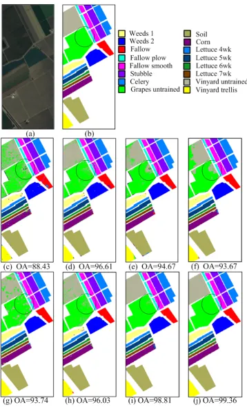
are discarded. Fig. 5 (a) and (b) show the color composite of the Indian Pines image
and the corresponding reference data, which contains sixteen reference classes from
different types of crops (e.g., corns, soybeans and wheat).
The Salinas image was also captured by AVIRIS sensor over the area of the Salinas
Valley, California. The image is of size 512×217×224, which has a spatial
resolution of 3.7 m per pixel. Same as in Indian Pines image, 20 water absorption
spectral bands are removed. Fig. 6 (a) and (b) show the color composite of the Salinas
The University of Pavia image was acquired with the ROSIS-03 sensor over the
campus at the University of Pavia, Italy. The image is of size 610×340×120, with a
spatial resolution of 1.3 m per pixel and a spectral coverage ranging from 0.43 to 0.86
μm [45]. Before the classification, 12 spectral bands were removed due to the high
noise. Fig. 7 (a) and (b) show the color composite of the University of Pavia image
and the corresponding reference data, which considers nine classes of interest.
B. Classification Results
In the experiments, the parameters for the proposed SC-MK and IntraSC-MK
methods are empirically selected and kept unchanged for the three test images. The
base superpixel number Lbase for the proposed SC-MK and IntraSC-MK methods are
chosen to 800. The parameter h in (9) is set 500. Setting larger h will give more power
for the neighboring superpixels, which improves the proposed method in large
homogeneous regions while decreasing the classification accuracies in the
heteregeous regions. When the h is vaired from 100 to 1000, the performance of the
proposed method changes very little in the three test images. The in (10) is set to
1. As indicated in [26], spatial kernel should be assigned with slightly larger weight,
compared with the spectral kernel. Therefore, for the IntraSC-MK method, the
spectral kernel weight Spec is set to 0.4, while the intra-superpixel kernel weight
IntraS
is chosen to 0.6. For the SC-MK method, the spectral kernel weight Spec,
intra-superpixel kernel weight IntraS, and inter-superpixel kernel weight InterS are
selected to 0.2, 0.4, 0.4, respectively. In the following subsection, the influences of the
SC-MK approach will be further analyzed. For the SVM method, the parameters C
and
are obtained by five-fold cross-validation. For the EMP, MLR-GCK andLORSAL-MLL methods, their parameters are set to the default values as in [23, 24,
41]. The parameters for the SRC and SVM-CK methods are tuned to reach their best
results in the experiments.
The first experiment was performed on the Indian Pines image. In this experiment,
training samples are randomly selected account for about 10% of the labeled reference
data (see the second column of the Table I). The visual classification results from
different classifiers are shown in Fig. 5. As can be observed, the SVM classifier that
only considers the spectral information exhibits very noisy estimations in its
classification map. By utilizing the spatial context of the HSI, the EMP,
LORSAL-MLL, SRC, SVM-CK, and MLR-GCK methods can deliver a smoother
appearance in their classification results. However, these approaches cannot
accurately classify pixels in the detailed and near-edge regions (e.g., ellipse regions in
Fig. 5). By contrast, the proposed superpixel based IntraSC-MK and SC-MK
approaches not only provide a smoother appearance, but also achieve more accurate
estimations in the detailed area (e.g., ellipse regions in Fig. 5). For the quantitative
comparison, our experiments adopt the overall accuracy (OA), average accuracy (AA),
and Kappa coefficient as the metrics to evaluate the classification results. Quantitative
results for various classifiers on the Indian Pines image are tabulated in Table I. Note
that, the classification accuracies reported in the Table I are the average results over
proposed IntraSC-MK and SC-MK methods perform better than the other compared
methods in terms of OA, AA, and the Kappa coefficient. In addition, we can observe
that the SC-MK method outperforms the IntraSC-MK method that only considers the
correlations within each superpixel. This demonstrates, that in addition to the
spectral-spatial information within each superpixel, further utilizing the spatial
information among superpixels in the SC-MK method can enhance the classification
performance.
The second and third experiments are conducted on Salinas and University of Pavia
images, respectively. In the experiment on the Salinas image, only 1% of the labeled
reference data were randomly selected as the training samples and the remaining 99%
of data as the test set (see the second column of Table II). In the experiment on the
University of Pavia image, as in some recent papers [46-48], a fixed number (200) of
training samples for each class were randomly selected as the training samples and the
rest as the test samples (see the second column of Table III). The selected training
samples account for about 4% of the whole labeled reference data, which provides a
challenging test set. The visual classification maps and quantitative results (averaged
over then experiments) obtained by various classifiers on the Salinas and University
of Pavia images are shown in Fig. 6 and 7, and Table II and III. As can be observed,
the proposed superpixel based SC-MK and IntraSC-MK classification methods
deliver better performances than the other compared classifiers, in terms of visual
quality and objective metrics. In addition, compared with the IntraSC-MK method
considers the correlations within and among superpixels, can further eliminate the
disturbances and improve the estimations (see the ellipse regions in Fig. 6 (i, j) and
Fig. 7 (i, j))
In the above experiments, all the programs are operated on a laptop computer with
an Intel (R) Corei7-3720 CPU 2.60 GHz and 16 GB of RAM. Table IV reports the the
computational time of each step for the proposed SC-MK method on the Indian Pines,
Salinas, University of Pavia images, respectively. As can be observed, the main
computational cost is occupied by the SVM training process. The step for creating the
superpixels does not consume much computational cost (0.09 second, 0.85 second,
and 1.35 second for the Indian Pines, Salinas, and University of Pavia, respectively).
This is because the PCA greatly reduces dimension of the HSI and the adopted
over-segmentation algorithm in [49] is very efficient. In addition, the main processes
for exploiting the information within and among superpixels (e.g., mean feature
within each superpixel, weighted average feature among superpixels, and multiple
kernels computations) also do not create much computational complexity. Note that,
since the SVM training process consumes too much computational cost, one of our
future works is to adopt the general-purpose graphics processing unit (GPU) to greatly
Fig. 5. Indian Pines image (a) Three-band color composite image. (b) Reference image, and the classification results (OA in %) obtained by the (c) SVM [7], (d) EMP [23], (e) SVM-CK [26], (f) LORSAL-MLL [41], (g) SRC [13], (h) MLR-GCK [41], (i) IntraSC-MK, (j) SC-MK methods.
TABLEI
CLASSIFICATION ACCURACIES OF INDIAN PINES IMAGE OBTAINED BY THE SVM [7],
EMP [23], SVM-CK [26], LORSAL-MLL [41], SRC [13], MLR-GCK [41], IntraSC-MK, AND SC-MK METHODS. CLASS-SPECIFIC ACCURACIES ARE IN
PERCENTAGE.
Class Training/Test SVM EMP SVM-CK
LORSAL-MLL SRC MLR-GCK IntraSC-MK SC-MK
Alfalfa 10/36 68.80 97.50 91.66 83.88 96.03 95.67 99.25 100
Corn-no till 143/1285 71.26 92.18 88.81 92.12 94.47 93.22 96.12 97.11
Corn-min till 83/747 73.91 88.47 86.66 89.05 92.35 95.92 97.08 97.65
Corn 24/213 62.28 79.24 83.38 95.58 92.55 94.00 96.93 97.82
Grass/Pasture 48/435 88.30 94.57 93.56 90.85 93.33 94.78 95.24 96.38
Grass/Trees 73/657 86.44 98.04 99.08 99.72 94.87 99.81 99.98 100
Grass/Pasture-mowed 10/18 88.07 61.24 93.33 92.22 88.88 98.14 97.24 100
Hay-windrowed 48/430 90.89 100 98.27 99.90 99.55 100 100 100
Oats 10/10 77.77 82.54 100 98.00 80.71 100 100 100
Soybeans-no till 97/875 74.42 92.57 86.66 91.86 91.93 91.17 93.69 93.35 Soybeans-min till 246/2209 78.79 92.58 92.10 95.89 96.36 97.91 98.48 99.02
Soybean-clean 59/534 69.31 88.76 83.80 97.15 90.61 95.13 95.88 97.80
Wheat 21/184 91.84 100 98.58 99.56 89.13 99.45 99.52 99.60
Woods 127/1138 92.60 99.24 97.82 97.66 98.21 99.39 99.70 99.98
Building-Grass-Trees-Drives 39/347 68.84 98.50 85.53 93.14 94.23 96.02 96.84 97.56 Stone-steel Towers 10/83 99.05 99.13 98.31 82.41 81.23 82.59 98.79 97.15
OA (Mean in %) 79.53 93.56 91.51 94.73 94.66 96.29 97.53 98.06
AA (Mean in %) 80.01 91.54 92.35 93.69 92.15 95.83 97.80 98.34
TABLEII
CLASSIFICATION ACCURACIES OF SALINAS IMAGE OBTAINED BY THE SVM [7], EMP
[23], SVM-CK [26], LORSAL-MLL [41], SRC [13], MLR-GCK[41], IntraSC-MK,
AND SC-MKMETHODS.CLASS-SPECIFIC ACCURACIES ARE IN PERCENTAGE.
Class Training/Test SVM EMP SVM-CK LORSAL-MLL SRC MLR-GCK IntraSC-MK SC-MK
Weeds_1 20/1989 99.74 99.84 99.09 99.44 100 98.75 100 100
Weeds_2 37/3689 99.01 99.76 99.37 99.95 99.98 99.35 100 100
Fallow 20/1956 91.05 93.15 98.69 99.78 97.61 97.54 99.92 100
Fallow plow 14/1380 97.04 98.49 99.00 98.34 83.24 98.84 98.44 98.62
Fallow smooth 27/2651 98.07 99.16 98.04 98.78 97.10 97.92 98.80 98.74
Stubble 40/3919 99.98 99.98 99.81 99.83 97.63 99.49 99.76 99.74
Celery 36/3543 98.89 99.92 99.34 99.66 99.57 99.51 99.92 99.92
Grapes 113/11158 75.96 92.96 89.86 90.76 88.61 92.21 99.32 99.81
Soil 62/6141 98.87 99.25 99.23 99.97 99.97 99.94 99.89 99.95
Corn 33/3245 88.86 93.37 95.00 94.15 96.11 96.46 96.49 97.65
Lettuce 4wk 11/1057 91.77 98.80 95.19 95.34 97.37 93.55 94.78 95.77
Lettuce 5wk 19/1908 95.75 96.53 99.84 99.99 95.52 99.88 98.59 100
Lettuce 6wk 9/907 94.78 98.01 99.12 97.83 95.08 98.38 98.11 98.15
Lettuce 7wk 11/1059 96.47 97.30 94.89 95.95 94.64 93.90 91.87 91.31
Vinyard untrained 73/7195 72.35 91.74 84.94 73.55 84.07 91.30 97.19 99.78
Vinyard trellis 18/1789 98.64 98.30 94.97 98.92 99.33 95.04 100 100
OA (Mean in %) 89.33 96.23 94.78 93.75 93.96 96.16 98.79 99.38
AA (Mean in %) 93.58 97.29 96.65 96.39 95.36 97.01 98.32 98.72
Kappa 0.88 0.95 0.94 0.93 0.93 0.96 0.99 0.99
C. Effect of the Number of Superpixels and Kernel Weights
In this section, the effect of the base superpixel number and kernel weights on the
performance of the proposed SC-MK method will be analyzed. In this analysis, the
numbers of training and test samples are selected to the same as in the above
experiments on the Indian Pines, Salinas, and University of Pavia images. Note that,
the reported accuracies for this analysis experiment are also the average results over
TABLE III
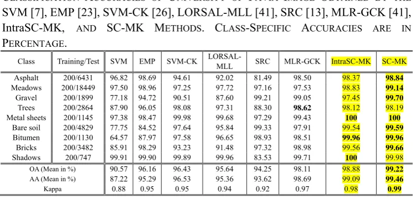
CLASSIFICATION ACCURACIES OF UNIVERSITY OF PAVIA IMAGE OBTAINED BY THE
SVM[7],EMP[23],SVM-CK[26],LORSAL-MLL[41],SRC[13],MLR-GCK[41], IntraSC-MK, AND SC-MK METHODS. CLASS-SPECIFIC ACCURACIES ARE IN
PERCENTAGE.
Class Training/Test SVM EMP SVM-CK
LORSAL-MLL SRC MLR-GCK IntraSC-MK SC-MK Asphalt 200/6431 96.82 98.69 94.61 92.02 81.49 98.50 98.37 98.84
Meadows 200/18449 97.50 98.96 97.25 97.72 97.16 97.53 98.83 99.14
Gravel 200/1899 77.18 94.72 90.51 87.60 99.21 99.05 97.45 99.70
Trees 200/2864 87.90 96.05 98.08 97.31 88.30 98.62 98.12 98.19 Metal sheets 200/1145 97.38 98.47 99.98 99.68 97.29 99.43 100 100
Bare soil 200/4829 77.75 84.52 97.64 95.84 99.33 97.91 99.54 99.59
Bitumen 200/1130 64.57 87.97 97.58 96.65 98.93 98.51 99.96 99.96
Bricks 200/3482 85.91 98.29 93.23 91.48 97.32 98.98 99.56 99.66
Shadows 200/747 99.91 99.90 99.89 99.96 83.53 99.71 100 99.98
OA (Mean in %) 90.57 96.16 96.43 95.64 94.25 98.11 98.88 99.22 AA (Mean in %) 87.22 95.29 96.53 95.36 93.62 98.69 99.09 99.46 Kappa 0.88 0.95 0.95 0.94 0.92 0.97 0.98 0.99
TABLEIV
THE RUN TIME (SECOND) FOR EACH STEP OF THE PROPOSED SC-MKMETHOD ON THE
INDIAN PINES,SALINAS, AND UNIVERSITY OF PAVIA IMAGES.
Indian Pines Salinas University of Pavia
Superpixel Creation 0.09 0.85 1.35
Mean Feature 0.08 0.41 0.44
Weighted Average Feature 0.15 1.89 2.02
SVM Training including kernels computation 149.05 36.86 128.65
SVM Test including kernels computation 9.83 9.91 42.31
Total 159.34 49.92 174.77
The base superpixel number was selected from 500 to 1600. Fig. 8 illustrates the
overall accuracies of the proposed SC-MK method under different base superpixel
numbers on the three test images. We can observe that, as the base superpixel number
varies from 500 to 1600, the overall accuracies of the proposed SC-MK method
generally show very good performances (overall accuracies are over 97.5%) on the
three test images. When the base superpixel number increases from 800 to 1600, the
overall accuracies of the proposed SC-MK method will slightly decrease on the three
[image:23.595.88.507.99.302.2]size of each superpixel will become small, and so the spatial information (e.g., in
large homogenous regions of Salinas image) will not be sufficiently exploited for
[image:24.595.143.466.168.336.2]classification.
Fig. 8. Effect of the base superpixel number on the proposed SC-MK algorithm over three HSI images.
To examine the influences of the kernel weights to the performance of the proposed
SC-MK method, the spectral kernel weight is first varied from 0 to 1, while the
intra-superpixel and inter-superpixel kernel weights are selected to the corresponding
equal values, as shown in the Fig. 9(a). If the spectral kernel weight is set to 1 or 0
(which means that only spectral information or spatial information of the superpixel is
utilized), the proposed SC-MK method does not show very good performances on the
three test images. This indicates that both the spectral information and the spatial
information of the superpixels should be utilized for the HSI classification. In addition,
when the spectral kernel weight goes from 0.2 to 0.9, the performances of the
proposed SC-MK method generally degrade on the three test images. This
demonstrates that comparatively large weight value should be assigned to the two
weight is fixed to 0.2, while the intra-superpixel and inter-superpixel kernel weights
are selected to the corresponding different values. As can be observed, if the
intra-superpixel kernel weight is set from 0.2 to 0.6, the performances of the proposed
SC-MK method are excellent and kept comparatively stable on the three test images.
This shows that the spectral information and spatial information within and among
superpixels should be all considered for the classification.
(a)
[image:25.595.129.502.256.639.2]
(b)
Fig. 9. Effect of the kernel weights on the proposed SC-MK algorithm on the three HSI images. (a) Effect of the spectral kernel weight; (b) Effect of the intra-superpixel and inter-superpixel kernel weights.
In this subsection, the effect of the number of training samples on several classifiers
will be examined on the Indian Pines, Salinas, and University of Pavia images. The
parameters for all the classifiers are kept the same as that in the Section IV. B. For the
Indian Pines and Salinas images, different percentages (from 2.5% to 30% for Indian
Pines and from 0.25% to 3% for Salinas) of the labeled data were randomly selected
as the training samples. For the University of Pavia image, various numbers (from 50
to 600 pixels for each class) of pixels were randomly chosen as the training set.
Fig. 10 illustrates the the overall classification accuracies (averaged over ten runs)
for each classifier under different number of training samples. We can observe that,
the performances for all the classifiers generally improve as the number of training
samples increase. Furthermore, the proposed SC-MK method consistently provides
superior performances over the other compared methods for all the test numbers of
[image:26.595.88.504.485.711.2]training samples.
V. CONCLUSIONS
In this paper, we present a superpixel-based classification via multiple kernels
(SC-MK) method for HSI classification. Instead of using fixed-size region as some
previous works, the SC-MK adopts the superpixel, whose size and shape can be
adaptively adjusted according to the spatial structures of the HSI. Then, the SC-MK
uses the multiple kernels to effectively exploit the spectral-spatial information within
and among superpixels. The experimental results on three real HSI images
demonstrate the superiority of the proposed SC-MK over several well-known
classifiers in terms of both visual quality on the classification map and quantitative
metrics.
In the experiments, the kernel weights were empirically selected to fixed values and
not optimized for each test image. Therefore, we will systematically research on how
to adaptively select the optimal kernel weights (e.g., based on the distributions of the
materials in local regions of the test image) for different images. In addition, our
future work will apply the superpixel based kernel model to other hyperspectral
applications (e.g., denoising, unmixing and object recognition).
ACKNOWLEDGMENT
We thank Dr. Jun Li and Dr. Ming-Yu Liu for providing the software for the
LORSAL-MLL and oversegmentation method, respectively, on their websites2,3. We
also thank the editors and all of the anonymous reviewers for their constructive
comments.
2http://www.lx.it.pt/~jun/.
REFERENCES
[1] M. Fauvel, Y. Tarabalka, J. A. Benediktsson, J. Chanussot, and J. C. Tilton, “Advances in spectral–spatial classification of hyperspectral images,” Proc. IEEE, vol. 101, no. 3, pp. 652–
675, Mar. 2013.
[2] L. Zhang, L. Zhang, D. Tao, and X. Huang, “Sparse transfer manifold embedding for hyperspectral target detection,” IEEE Trans. Geosci. Remote Sens., vol. 52, no. 2, pp.
1030-1043, Feb. 2014.
[3] B. Du and L. Zhang, “Random-selection-based anomaly detector for hyperspectral imagery,”
IEEE Trans. Geosci. Remote Sens., vol. 49, no. 5, pp. 1578-1589, Apr. 2011.
[4] J. M. Bioucas-Dias, A. Plaza, N. Dobigeon, M. Parente, Q. Du, P. Gader, and J. Chanussot, “Hyperspectral unmixing overview: Geometrical, statistical, and sparse regression-based approaches,” IEEE J. Sel. Topics Appl. Earth Observ. Remote Sens., vol. 5, no. 2, pp. 354-379,
Apr. 2012.
[5] N. Younan, S. Aksoy, and R. King, “Foreword to the special issue on pattern recognition in remote sensing,” IEEE J. Sel. Topics Appl. Earth Observ. Remote Sens., vol. 5, no. 5, pp.
1331–1334, Oct. 2012.
[6] V. Vapnik, The nature of statistical learning theory: Berlin, Germany: Springer-Verlag, 1995.
[7] F. Melgani and L. Bruzzone, “Classification of hyperspectral remote sensing images with support vector machines,” IEEE Trans. Geosci. Remote Sens., vol. 42, no. 8, pp. 1778-1790,
Aug. 2004.
[8] D. Böhning, “Multinomial logistic regression algorithm,” Ann. Inst. Stat. Math., vol. 44, no. 1,
pp. 197-200, Mar. 1992.
[9] J. Li, J. M. Bioucas-Dias, and A. Plaza, “Spectral–spatial hyperspectral image segmentation using subspace multinomial logistic regression and Markov random fields,” IEEE Trans. Geosci. Remote Sens., vol. 50, no. 3, pp. 809-823, Mar. 2012.
[10] J. Li, J. M. Bioucas-Dias, and A. Plaza, “Semisupervised hyperspectral image segmentation using multinomial logistic regression with active learning,” IEEE Trans. Geosci. Remote Sens.,
vol. 48, no. 11, pp. 4085-4098, Nov. 2010.
[11] B. Du and L. Zhang, “Target detection based on a dynamic subspace,” Pattern Recogn., vol.
47, no. 1, pp. 344-358, Jan. 2014.
[12] B. Du and L. Zhang, “Random-selection-based anomaly detector for hyperspectral imagery,”
IEEE Trans. Geosci. Remote Sens., vol. 49, no. 5, pp. 1578–1589, May 2011.
[13] Y. Chen, N. M. Nasrabadi, and T. D. Tran, “Hyperspectral image classification using dictionary-based sparse representation,” IEEE Trans. Geosci. Remote Sens., vol. 49, no. 10, pp.
3973-3985, Oct. 2011.
[14] U. Srinivas, Y. Chen, V. Monga, N. M. Nasrabadi, and T. D. Tran, “Exploiting sparsity in hyperspectral image classification via graphical models,” IEEE Geosci. Remote Sens. Lett.,
vol. 10, no. 3, pp. 505-509, May 2013.
[15] Y. Chen, N. M. Nasrabadi, and T. D. Tran, “Hyperspectral image classification via kernel sparse representation,” IEEE Trans. Geosci. Remote Sens., vol. 51, no. 1, pp. 217-231, Jan.
2013.
[16] B. Du and L. Zhang, “A discriminative metric learning based anomaly detection method,”
IEEE Trans. Geosci. Remote Sens., vol. 52, no. 11, pp. 6844-6857, May 2014.
target recognition,” IEEE Geosci. Remote Sens. Lett., vol. 5, no. 4, pp. 625-629, Oct. 2008.
[18] L. Zhang, Y. Zhong, B. Huang, J. Gong, and P. Li, “Dimensionality reduction based on clonal selection for hyperspectral imagery,” IEEE Trans. Geosci. Remote Sens., vol. 45, no. 12, pp.
4172-4186, Dec. 2007.
[19] H. Li, Z. Ye, and G. Xiao, “Hyperspectral Image Classification Using Spectral–Spatial Composite Kernels Discriminant Analysis,” IEEE J. Sel. Topics Appl. Earth Observ. Remote Sens., In Press, 2015.
[20] Q. Shi, L. Zhang, and B. Du, “Semisupervised discriminative locally enhanced alignment for hyperspectral image classification,” IEEE Trans. Geosci. Remote Sens., vol. 51, no. 9, pp.
4800-4815, Feb. 2013.
[21] G. Camps-Valls and L. Bruzzone, Kernel Methods for Remote Sensing Data Analysis: New
York: Wiley, 2009.
[22] J. Li, I. Dópido, P. Gamba, and A. Plaza, “Complementarity of discriminative classifiers and spectral unmixing techniques for the interpretation of hyperspectral images,” IEEE Trans. Geosci. Remote Sens., In Press, 2015.
[23] J. A. Benediktsson, J. A. Palmason, and J. R. Sveinsson, “Classification of hyperspectral data from urban areas based on extended morphological profiles,” IEEE Trans. Geosci. Remote Sens., vol. 43, no. 3, pp. 480-491, Mar. 2005.
[24] J. Li, P. R. Marpu, A. Plaza, J. M. Bioucas-Dias, and J. A. Benediktsson, “Generalized composite kernel framework for hyperspectral image classification,” IEEE Trans. Geosci. Remote Sens., vol. 51, no. 9, pp. 4816-4829, Sept. 2013.
[25] Y. Tarabalka, J. A. Benediktsson, and J. Chanussot, “Spectral–spatial classification of hyperspectral imagery based on partitional clustering techniques,” IEEE Trans. Geosci. Remote Sens., vol. 47, no. 8, pp. 2973-2987, Aug. 2009.
[26] G. Camps-Valls, L. Gomez-Chova, J. Muñoz-Marí, J. Vila-Francés, and J. Calpe-Maravilla, “Composite kernels for hyperspectral image classification,” IEEE Geosci. Remote Sens. Lett.,
vol. 3, no. 1, pp. 93-97, Jan. 2006.
[27] G. Mori, X. Ren, A. A. Efros, and J. Malik, “Recovering human body configurations: Combining segmentation and recognition,” in Proc. IEEE Conf. Comput. Vis. Pattern Recog.,
2004, pp. II-326-II-333.
[28] R. Achanta, A. Shaji, K. Smith, A. Lucchi, P. Fua, and S. Susstrunk, “SLIC superpixels compared to state-of-the-art superpixel methods,” IEEE Trans. Pattern Anal. Mach. Intell., vol.
34, no. 11, pp. 2274-2281, Nov. 2012.
[29] M.-Y. Liu, O. Tuzel, S. Ramalingam, and R. Chellappa, “Entropy rate superpixel segmentation,” in Proc. IEEE Conf. Comput. Vis. Pattern Recog., 2011, pp. 2097-2104.
[30] G. Zhang, X. Jia, and N. M. Kwok, “Super pixel based remote sensing image classification with histogram descriptors on spectral and spatial data,” in Proc. IEEE Int. Geo. Remot. Sens. Symp., 2012, pp. 4335-4338.
[31] J. Liu, W. Yang, S. Tan, and Z. Wang, “Remote sensing image classification based on random projection super-pixel segmentation,” in Proc. SPIE, 2013, pp. 89210T-89210T-7.
[32] Z. Sun, C. Wang, H. Wang, and J. Li, “Learn multiple-kernel SVMs for domain adaptation in hyperspectral data,” IEEE Geosci. Remote Sens. Lett., vol. 10, no. 5, pp. 1224-1228, Jun.
2013.
learning for classification in hyperspectral imagery,” IEEE Trans. Geosci. Remote Sens., vol.
50, no. 7, pp. 2852-2865, Jul. 2012.
[34] V. N. Vapnik, Statistical learning theory vol. 2: Wiley New York, 1998.
[35] I. Jolliffe, Principal component analysis: Wiley Online Library, 2005.
[36] R. C. Gonzalez and R. E. Woods, Digital image processing: Prentice Hall, 2009.
[37] G. L. Nemhauser, L. A. Wolsey, and M. L. Fisher, “An analysis of approximations for maximizing submodular set functions,” Math. Program., vol. 14, no. 1, pp. 265-294, Jan.
1978.
[38] J. Liu, Z. Wu, Z. Wei, L. Xiao, and L. Sun, “Spatial-spectral kernel sparse representation for hyperspectral image classification,” IEEE J. Sel. Topics Appl. Earth Observ. Remote Sens., vol.
6, no. 6, pp. 2462-2471, Apr. 2013.
[39] K. He, J. Sun, and X. Tang, “Guided image filtering,” IEEE Trans. Pattern Anal. Mach. Intell.,
vol. 35, no. 6, pp. 1397-1409, June 2013.
[40] L. Fang, S. Li, R. McNabb, Q. Nie, A. Kuo, C. Toth, J. A. Izatt, and S. Farsiu, “Fast Acquisition and Reconstruction of Optical Coherence Tomography Images via Sparse Representation,” IEEE Trans. Med. Imag., vol. 32, no. 11, pp. 2034-2049, Nov. 2013.
[41] J. Li, J. M. Bioucas-Dias, and A. Plaza, “Hyperspectral image segmentation using a new Bayesian approach with active learning,” IEEE Trans. Geosci. Remote Sens., vol. 49, no. 10,
pp. 3947-3960, Oct. 2011.
[42] C.-C. Chang and C.-J. Lin, “LIBSVM: a library for support vector machines,” ACM Trans. Intell. Systems Technology, vol. 2, no. 3, pp. 27:1–27:27, July 2011.
[43] M. Dalla Mura, J. Atli Benediktsson, B. Waske, and L. Bruzzone, “Extended profiles with morphological attribute filters for the analysis of hyperspectral data,” Int. J. Remote Sens., vol.
31, no. 22, pp. 5975-5991, Jul. 2010.
[44] J. A. Gualtieri and R. F. Cromp, “Support vector machines for hyperspectral remote sensing classification,” in Proc. SPIE, 1999, pp. 221-232.
[45] A. Plaza, J. A. Benediktsson, J. W. Boardman, J. Brazile, L. Bruzzone, G. Camps-Valls, J. Chanussot, M. Fauvel, P. Gamba, and A. Gualtieri, “Recent advances in techniques for hyperspectral image processing,” Remote Sens. Environ., vol. 113, pp. S110-S122, Sep. 2009.
[46] J. Li, H. Zhang, Y. Huang, and L. Zhang, “Hyperspectral image classification by nonlocal joint collaborative representation with a locally adaptive dictionary,” IEEE Trans. Geosci. Remote Sens., vol. 52, no. 6, pp. 3707-3719, June 2014.
[47] B. Song, J. Li, M. D. Mura, P. Li, A. Plaza, J. M. B. Dias, J. A. Benediktsson, and J. Chanussot, “Remotely sensed image classification using sparse representations of morphological attribute profiles,” IEEE Trans. Geosci. Remote Sens., vol. 52, no. 8, pp. 5122-5136, Aug.2014.
[48] R. Ji, Y. Gao, R. Hong, Q. Liu, D. Tao, and X. Li, “Spectral-spatial constraint hyperspectral image classification,” IEEE Trans. Geosci. Remote Sens., vol. 52, no. 3, pp. 1811-1824, Mar.
2014.
Leyuan Fang (S’10-M’14) received the B.S. degree in electrical engineering from
Hunan University of Science and Technology, China, in 2008. He joined the College of Electrical and Information Engineering, Hunan University, China, in 2008, for the Ph.D. degree program.
Since September 2011, he has been a Visiting Ph.D. Student in the Department of Ophthalmology, Duke University, Durham, NC, supported by the China Scholarship Council. His research interests include sparse representation and multiresolution analysis in remote sensing and medical image processing.
Mr. Fang has won the Scholarship Award for Excellent Doctoral Student granted by Chinese Ministry of Education in 2011.
Shutao Li (M’07-SM’15) received his B.S., M.S., and Ph.D. degrees in electrical
engineering from the Hunan University, in 1995, 1997, and 2001, respectively. He joined the College of Electrical and Information Engineering, Hunan University, in 2001. He was Research Associate in the Department of Computer Science, Hong Kong University of Science and Technology, from May 2001 to October 2001. From November 2002 to November 2003, he was a postdoctoral fellow at the Royal Holloway College, University of London, working with Prof. John Shawe-Taylor. During April 2005 to June 2005, he has visited the Department of Computer Science, Hong Kong University of Science and Technology as a visiting professor. Now, he is a full professor with the College of Electrical and Information Engineering, Hunan University. He has authored or coauthored more than 160 refereed papers. His professional interests are compressive sensing, sparse representation, image processing, and pattern recognition.
Dr. Li is an Associate Editor of the IEEE Transactions on Geoscience and Remote Sensing (TGRS), a member of the Editorial Board of the journal Information Fusion and the Sensing and Imaging. He was a recipient of two Second-Grade National Awards at the Science and Technology Progress of China in 2004 and 2006.
Wuhui Duan received the B.S. degree in the College of Electrical and Information
Engineering, Hunan University, China, in 2012. She continues working toward the M.S. degree in Hunan University now. Her research interest is spectral-spatial hyper spectral image classification.
Jinchang Ren received the PhD degree in Electronic Imaging and Media
Communication from the University of Bradford, United Kingdom in 2009. Before that, he obtained M.Eng. in Image Processing and Pattern Recognition and B. Eng. in Computer Software from Northwestern Polytechnical University, China, in 1997 and 1992, respectively.
including University of Bradford, University of Surrey, Kingston University and University of Abertay, Dundee.
Dr. Ren has published over 100 peer-reviewed research papers in prestigious international journals and conferences, including IEEE Trans. Image Processing, IEEE Trans. Circuits & Systems for Video Technology, IEEE Trans. Multimedia, IEEE Trans. System Man and Cybernetics, Computer Vision and Image Understanding, etc. as well as British Machine Vision Conference, Int. Conf. Image Proc., Int. Conf. Multimedia and Expo, Visual Information Engineering and book series of LNCS, etc. His research interests include: pattern recognition; human-computer interaction; visual surveillance; archive restoration; motion estimation; hyperspectral imaging.
Jón Atli Benediktsson (S’84-M’90-SM’99-F’04) received the Cand.Sci. degree in
electrical engineering from the University of Iceland, Reykjavik, Iceland, in 1984 and the M.S.E.E. and Ph.D. degrees in electrical engineering from Purdue University, West Lafayette, IN, in 1987 and 1990, respectively.
Currently, he is Rector at the University of Iceland. His research interests are in remote sensing, image analysis, pattern recognition, biomedical analysis of signals, and signal processing, and he has published extensively in those fields. He is a cofounder of the biomedical startup company Oxymap.
![Fig. 5. Indian Pines image (a) Three-band color composite image. (b) Reference image, and the classification results (OA in %) obtained by the (c) SVM [7], (d) EMP [23], (e) SVM-CK [26], (f) LORSAL-MLL [41], (g) SRC [13], (h) MLR-GCK [41], (i) IntraSC-MK,](https://thumb-us.123doks.com/thumbv2/123dok_us/1586886.111346/19.595.65.534.536.759/indian-composite-reference-classification-results-obtained-lorsal-intrasc.webp)
![Fig. 7. University of Pavia image (a) Three-band color composite image. (b) Reference image, and the classification results (OA in %) obtained by the (c) SVM [7], (d) EMP [23], (e) SVM-CK [26], (f) LORSAL-MLL [41], (g) SRC [13], (h) MLR-GCK [41], (i) Intra](https://thumb-us.123doks.com/thumbv2/123dok_us/1586886.111346/22.595.119.480.72.587/university-composite-reference-classification-results-obtained-lorsal-intra.webp)