A higher order control volume based finite element method to prodict the deformation of heterogeneous materials

A higher order control volume based finite element method to

predict the deformation of heterogeneous materials.

A. J. Beveridge, M. A. Wheel and D. H. Nash

Department of Mechanical and Aerospace Engineering, University of Strathclyde, Glasgow, UK, G4 0LT

Abstract

Materials with obvious internal structure can exhibit behaviour, under loading, that cannot be described by classical elasticity. It is therefore important to develop computational tools in-corporating appropriate constitutive theories that can capture their unconventional behaviour. One such theory is micropolar elasticity. This paper presents a linear strain control volume finite element formulation incorporating micropolar elasticity. Verification results from a mi-cropolar element patch test as well as convergence results for a stress concentration problem are included. The element will be shown to pass the patch test and also exhibit accuracy that is at least equivalent to its finite element counterpart.

Keywords: control volume finite element method, heterogeneous materials, micropolar

elasticity

1. Introduction

The understanding of the response of heterogeneous materials under loading, particularly the numerical modelling of this, has become an engineering challenge due to the increased use of heterogeneous materials in structural applications [1]. For example, polymeric and metallic foams, particularly as part of sandwich panels, are now being used more extensively in both au-tomotive and aerospace applications because of the weight saving they afford [1]. It is an active research area to find constitutive models that can describe the elastic response of heterogeneous materials as they are often endowed with enhanced mechanical behaviour. This may include so called size effects [2], which recognize the dependence of the enhanced mechanical behaviour upon the size of the material domain.

Micropolar elasticity is endowed with additional independent micro rotations which are as-sociated with additional stress measures termed couple stresses. These enable the complimen-tary shear stress requirement of classical elasticity to be relaxed; the couple stresses balance the differential element. The couple stresses also have intrinsic length scales associated with them. With this additional degree of freedom micropolar elasticity predicts elastic behaviour that is not predicted by classical elasticity. For example the dispersion of stress waves, a dependence of stress concentration factor upon discontinuity size and a size stiffening of smaller samples in bending and torsion are all predicted. These size effects have been identified experimentally.

Koh[3]. They formulated a bi-linear triangular element with linear displacement and linear mi-cro rotation fields. Although no numerical results are presented they note that their purpose is to bring micropolar elasticity and its associated micro continuum models from “ one of abstrac-tion to that of reality”. The nature of micro continuum theories is complex and therefore very few analytical solutions exist. Goldberg, Baluch, Korman and Koh [4], in a later work, states that the finite element method is used “in order to alleviate the inherent complexity” involved in solving the system of governing equations. This later work presents an FEM for the bending of micropolar plates using a 3 noded triangular element with 15 degrees of freedom; transverse displacement, rotation and micro rotation.

Nakamura, Benedict and Lakes [5] present another bi-linear triangular element for or-thotropic micropolar elasticity. Results are shown for the estimation of stress concentration factors of a circular hole in an infinite plate, for which an analytical solution exists. The model is capable of identifying the size effect, although there is an error in the computed value that appears to be dependent upon the coupling number; the larger the value of the coupling number, which is a constitutive property governing the antisymmetry of the shear stresses in micropolar elasticity, the greater the error. This issue is identified in other works [6, 7]. In a later work Nakamura and Lakes [8] present a finite element analysis package called MIRACS (Micro ro-tation and couple stress) which is used to investigate Saint-Venant end effects in micropolar elastic materials. A 3 node constant strain triangular element, a 4 node isoparametric element and an 8 node isoparametric element make up the package. Further plane elements have been published [9, 10, 6, 11]. The quadratic element of Providas and Kattis [6] is the most accurate plane finite element to date. In [6], a patch test is presented to robustly assess the published element.

Wheel [7] departs from the standard finite element procedure to publish a constant strain planar control volume method. The constant strain control volume element shows enhanced performance in the patch test proposed by Providas and Kattis. It returns exact predictions of displacements, rotations and stresses for all three proposed tests where as the finite element formulations of Providas and Kattis return exact solutions in the first two tests. In the third test, however, predictions, although accurate, were acknowledged to be approximate rather than exact. Control volume (CV) methods, allowing the same versatility with complex geometries, have been developed initially for both computational fluid mechanics and more recently struc-tural analysis applications [12, 13, 14, 15]. This recent development has been motivated by the desire to analyse fluid structure interactions and more general multiphysics problems within a unified computational framework [7]. One particular control volume method, the control vol-ume finite element method (CVFEM), is constructed upon the same mesh as the finite element discretisation resulting in a so called vertex centred method [7]. Recently a vertex centred CVFEM for classical elasticity has been shown to provide better convergence, than the equiva-lent FEM, for a plane triangular element with both rotation and translation degrees of freedom [16]. The CV method has also been applied to plate bending problems where both the cell centred [17] and vertex centred methods [18] have shown to be locking free for thick and thin Mindlin plates. In recent developments control volumes have been used in the structural analy-sis of radio frequency MEMS devices [19] and in the analyanaly-sis of the micromechanics of periodic materials [20].

moti-vation for this was to develop an inverse method to identify micropolar constitutive properties. Micropolar constitutive properties are difficult to identify experimentally and few properties have been published. The higher order element, set out here, has been used in an iterative inverse procedure to identify the micropolar constitutive properties of model two phase metal composite beam [21] and polymer ring [22] samples. This inverse procedure has produced a simple method to determine constitutive properties. Combining this with the available mi-cropolar elements it is hoped that this will encourage mimi-cropolar elasticity as a method for the computational prediction of deformations in heterogeneous materials.

Presented in this paper will be the formulation of this element. In addition its performance will be compared to published elements and shown to be at least equivalent. Before the for-mulation of the element is presented the mathematical theory of micropolar elasticity will be briefly described.

2. Micropolar Elasticity

Micropolar elasticity is one of the higher order non-local theories of Eringen [23]. It is endowed with an additional micro rotation vector that removes the restriction presented within classical elasticity that the shear stresses are symmetric. It is a general model and will converge to both classical elasticity and couple stress theory [24]; the conditions under which this occurs are discussed later. The three dimensional stress tensors of linear micropolar elasticity are introduced here and the significance of the associated constitutive properties are discussed. Following this the two dimensional formulations of plane stress and plane strain, used in the element formulations, will be presented.

2.1. Generalised Linear Micropolar Elasticity

Linear micropolar elasticity takes into account the deformation of the microstructure by introducing a length scale dependent couple stress,m, and an additional degree of freedom, the micro rotationφ. For a linear elastic isotropic micropolar material the force stress tensor, τij, and couple stress tensor,mij, respectively are [25],

τij =λεkkδij + (2µ∗_{+κ)εij +κeijk(θk−φk) (1)}

mij =αφk,kδij +βφi,j +γφj,i (2) The repeated indices denote summation over the range (i, j, k= 1,2,3), δij is the Kronecker delta andeijk is the permutation tensor. These are defined in the following way:

δij =

(

1, ifi=j

0, ifi6=j (3)

eijk =

    

+1, ifijk is an even permutation of (1,2,3)

−1, ifijk is an odd permutation of (1,2,3) 0, otherwise

(4)

elastic constants. The micropolar shear modulus,µ∗_{, is related to the classical shear modulusµ} by,

µ=µ∗₊κ

2 (5)

The macro rotation and strain tensor are,

θi = 1

2eijkuk,j (6)

εij = 1

2(ui,j+uj,i) (7)

respectively, whereuis the displacement vector. The six elastic constants can be expressed in terms of seven engineering constants [24]:

Em = (2µ

∗_{+κ) (3λ+ 2µ}∗_+κ)

(2λ+ 2µ∗+κ) (8)

Gm =µ∗₊κ

2 (9)

νm = λ

(2λ+ 2µ∗ +κ) (10)

l2t =

(β+γ)

(2µ∗+κ) (11)

l2 b =

γ

2 (2µ∗_+κ) (12)

N2 = κ

2 (µ∗_+κ) (13)

Ψ = (β+γ)

(α+β+γ) (14)

whereEmis the micropolar Young’s modulus,Gm the observed micropolar shear modulus,νm

the micropolar Poisson’s ratio,ltthe characteristic length of torsion,lbthe characteristic length of bending, N the coupling number and Ψ the polar ratio. The micropolar elastic constants,

Em,Gm andνmgovern uniform dilitational and distortional deformation in the same way as in classical elasticity theory. The characteristic lengths of torsion and bending dictate the length scale of the size effects. The coupling number controls the antisymmetry of the shear stresses. The polar ratio is similar to Poisson’s ratio but relates orthogonal microrotations rather than dilatational strains. The micropolar theory contains two limits. Ifα, β, γ andκare set to zero, the solid will behave in a classical manner. Alternatively, if the coupling number N is set to 1 then the material will behave as in couple stress theory [24], where the micro rotation is no longer kinematically distinct from the macro rotation.

2.2. Two Dimensional Formulations

equations for the balance of stress and couple stress, see figure 1, are respectively;

τij,i+pj = 0 (15)

and

mi3,i+eij3τij +q3 = 0 (16)

where the repeated indices denote summation over the range(i, j = 1,2), pj are body forces per unit volume andq3 represents a body couple per unit volume. Expanding the equilibrium equations for Cartesian coordinates,(i, j =x, y)and setting the free index3toz gives;

τxx,x+τyx,y+px= 0 (17)

τyy,y +τxy,y+py = 0 (18)

mxz,x+myz,y+τxy −τyx+qz = 0 (19) The linear constitutive equations can be expressed as,

τij =λεkkδij + (µ∗_{+κ)εij +µ}∗_{εji (20)}

mij =αφk,kδij +βφi,j +γφj,i (21) where the repeated indices denote summation over the range(i, j, k = 1,2,3). Introducing a modified strain displacement relationship,

εij =uj,i+ejikφk (22)

which when expanded for Cartesian coordinates(i, j, k=x, y, z)gives,

   

εxx εyy εyx εxy

   

=

   

u,x v,y u,y+φz v,x−φz

   

(23)

whereuandv are the displacement components of thexandydirections respectively. The dis-placement gradientsu,y,v,xare associated with the symmetric component of the shear stresses,

τs, while the micro rotationφzis due to the antisymmetric component of the shear stresses,τa, see figure 2. The constitutive equations are now modified to account for the specific assump-tions associated with the plane stress and plane strain cases.

2.2.1. Plane Strain

stress,     τxx τyy τyx τxy     =    

λ+ 2µ∗_{+κ λ 0 0}

λ λ+ 2µ∗_{+κ 0 0}

0 0 µ∗ _{+κ µ}∗

0 0 µ∗ _µ∗_+κ

        εxx εyy εyx εxy     (24)

and couple stress,

mxz myz = γ 0 0 γ φz,x φz,y (25)

These can be reformulated in term of the engineering material constantsEm,vm,lbandN from equations (8),(10),(12) and (13) respectively as,

    τxx τyy τyx τxy     = Em

(1 +νm)

      

(1−νm)

(1−2νm)

νm

(1−2νm) 0 0

νm

(1−2νm)

(1−νm)

(1−2νm) 0 0

0 0 ₂₍₁1

−N2)

(1−2N2)

2(1−N2)

0 0 (1−2N

2

)

2(1−N2)

1 2(1−N2)

           εxx εyy εyx εxy     (26) mxz myz =

" _2Eml2_b

(1+νm) 0 0 2Eml2_b

(1+νm)

# φz,x φz,y (27)

An alternative relationship between the shear stresses and the shear strains can be formulated by introducing a new constitutive parameter, the coupling factor,a, where,

N2 = a

1 +a (28)

Then expressing the shear modulusGmas

Gm = Em

2 (1 +νm) (29)

allows the shear stresses to be related to the shear strains in the simpler form,

τyx τxy =Gm

1 +a 1−a

1−a 1 +a

εyx εxy

(30)

2.2.2. Plane Stress

In plane stress theory it is assumed that the stress in the z direction is zero and again that the micro rotations about thexandyaxes are zero. Thereforeτzz =τxz =τyz =τzx=τzy= 0

andφx =φy = 0. As the assumptions with respect to the couple stress are unchanged between plane stress and plane strain the constitutive relationships are unchanged from equations (25) and (27). However the modified force stress constitutive relationships are,

    τxx τyy τyx τxy     =     

(2µ∗_+κ)(2λ+2µ∗_+κ)

λ+2µ∗_+κ

λ(2µ∗_+κ)

λ+2µ∗_+κ 0 0

λ(2µ∗_+κ)

λ+2µ∗_+κ

(2µ∗_+κ)(2λ+2µ∗_+κ)

λ+2µ∗_+κ 0 0

0 0 µ∗_{+κ µ}∗

0 0 µ∗ _µ∗_+κ

which can once more be expressed in terms of the engineering constants,     τxx τyy τyx τxy     = Em

(1−ν2 m)      

1 νm 0 0

νm 1 0 0

0 0 (1−νm)

2(1−N2)

(1−νm)(1₋2N2)

2(1−N2)

0 0 (1−νm)(1−2N

2

)

2(1−N2)

(1−νm)

2(1−N2)

          εxx εyy εyx εxy     (32)

3. Micropolar Linear Strain Triangular Element

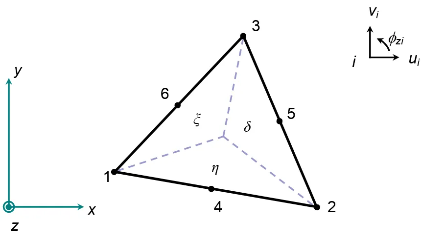
The formulation of the quadratic displacement, linear strain, triangular micropolar plane stress/strain control volume finite element (CV-MPLST) begins with a 6 noded, 18 degrees of freedom element consisting of a straight edged triangle with 3 vertex and 3 midside nodes, figure 3. The displacements in the x direction, u, y direction, v, and micro rotation φz are interpolated over the element with a complete quadratic polynomial from the nodal degrees of freedom,ui,viandφziwhere the indexi= 1 : 6refer to the element nodes.

u=P6

i=1N

i_{ui v =}P6

i=1N

i_{vi φz =}P6

i=1N

i_{φzi (33)}

The superscriptiindicates position within the array. The shape functions Ni _{are functions of}

the natural area coordinates(δ, ξ, η)[26]. The natural area coordinates are related to the element vertex coordinates,(x1, x2, x3)and(y1, y2, y3), and global coordinate(x, y)by

x=δx1+ξx2+ηx3

y=δy1+ξy2+ηy3 (34)

Vector[N_{]of shape functions is}

[N_{] = δ(2δ−1) ξ(2ξ−1) η(2η−1) 4δξ 4ξη 4ηδ (35)}

The displacement vector{d_}is

{d_}=

ui vi φzi T

for i= 1 : 6 (36)

The unknown element displacements and micro rotations are related to the nodal degrees of freedom by   u v φz 

= [N]{d} (37)

The strain vector{ε}is related to the element displacements by

{ε}=         εxx εyy εyx εxy φz,x φz,y         =         u,x v,y u,y+φz v,x−φz

φz,x φz,y         =          ∂

∂x 0 0

0 ∂

∂y 0 ∂

∂y 0 1

0 ∂

∂x −1

0 0 ∂

∂x

0 0 _∂y∂

and the stress vector{τ}is related to the strain vector by {τ}=         τxx τyy τyx τxy mxz myz        

= [D_{]{ε} (39)}

whereD_{refers to the constitutive matrix defined in section 2.2 with the inclusion of the}

consti-tutive properties for the micro rotation. For example in the plane stress case;

[D_{] =}

       

λ+ 2µ∗ _{+κ λ 0 0 0 0}

λ λ+ 2µ∗ _{+κ 0 0 0 0}

0 0 µ∗_{+κ µ}∗ _{0 0}

0 0 µ∗ _µ∗_{+κ 0 0}

0 0 0 0 γ 0

0 0 0 0 0 γ

        (40)

Differentiating the shape functions with respect to the spatial coordinates,

N,x N,y = 1 2A

y23N,δ+y31N,ξ+y12N,η −x23N,δ−x31N,ξ−x12N,η

(41)

whereyij = yi −yj, i = 1,2,3represents the vertex node numbers and(xi, yi)are the vertex node coordinates.Ais the area of the triangular element. The derivatives of the shape functions with respect to the area coordinates are

N,δ =

4δ−1 0 0 4ξ 0 4η

(42)

N,ξ =

0 4ξ−1 0 4δ 4η 0

(43)

N,η =

0 0 4η−1 0 4ξ 4δ

(44)

These are used in the formulation of the strain displacement matrix[B_{] which relates the}

un-known nodal degrees of freedom to the element strain vector{ε}thus :

{ε}= [B_]

  ui vi φzi 

 for i= 1 : 6 where [B] =         Ni

,x 0 0

0 Ni

,y 0 Ni

,y 0 Ni

0 Ni

,x −Ni

0 0 Ni

,x

0 0 Ni

,y         (45)

the element stress resultants can then be related to the unknown nodal displacements by

{τ}= [D_{] [}B_]{d_{} (46)}

briefly.

3.1. Finite Element Procedure

In the case of the standard finite element procedure the stiffness matrix is calculated from,

k_{FEM= 2A}

Z 1

0

Z 1−η

0

BTD_bB_{dξdη (47)}

in the usual way. To enable a comparison between the FEM and CVFEM formulations based upon the triangular element, this equation (47) is evaluated by symbolic integration using the Maple kernel of MATLAB.

While the finite element formulation developed here is based upon the standard approach it differs slightly in that the Maple kernel provides exact analytical expressions for each term in (47) rather than approximations based on numerical integration. This provides a fair basis for comparison since the CVFEM procedure employs exact integration.

3.2. Control Volume Formulation

A dual mesh of interconnecting control volumes is set up on the finite element mesh. Each control volume is centred upon a node of the element, see figure 4. The control volumes are constructed on an element by element basis as shown in figure 5. Table 1 shows the coordi-nates of the control volume vertices expressed in terms of the area coordicoordi-nates of the triangular element, although other coordinates could of course be used.

The equilibrium equations, section 2.2 and equations (17), (18) and (19), are setup for each control volume where the stress resultants acting upon the boundaries of the control volume are equilibrated against any body loadings imposed upon the control volume thus:

n

X

k=1 Fk

x +pxAv = 0 (48)

n

X

k=1

Fyk+pyAv = 0 (49)

n

X

k=1 Mk

z +qzAv = 0 (50)

whereFk

x and Fyk are components of the force resultants acting upon control volume face k, Mk

z is the couple resultant,Av is the area of the control volume andn is the number of control

volume faces around the finite element vertex or midside node that the control volume is centred on. The force and couple resultants are computed by analytical integrating the functions of the stress variations within the finite element along each control volume edge, figure 6. As each control volume face lies entirely within a given element, this is performed without storing any information relating to CV connectivity and is done on an element by element basis, giving a stiffness matrix for each triangular element. This allows the global stiffness matrix to be assem-bled in an identical manner to the finite element method. The discrete equilibrium equations for one control volume face are,

Fmn

x =

Z

τxxcosθmndr+

Z

Fmn

y =

Z

τyysinθmndr+

Z

τxycosθmndr (52)

Mmn zi =

Z

mxzcosθmndr+

Z

myzsinθmndr+

Z

x′τxycosθmndr−

Z

y′τyxsinθmndr (53)

where

cosθmn=−ymn

lmn xmn =xm−xn sinθmn = xmn

lmn ymn=ym−yn

lmn = (x2

mn+ymn2 ) 1 2

(54)

andmand ndenote the vertices of the control volume edge, figure 6. Moment arm functions

x′

andy′

are the distances from the element vertex or midside nodei, that the control volume is centred upon, and the edge itself so

x′

=xe−xi

y′ =ye−yi (55)

(xi, yi)being the coordinates of the centre node of the control volume and(xe, ye)are functions of the area coordinates relating any point within the element to the associated vertex nodes thus:

xe =δx1+ξx2+ηx3

ye=δy1+ξy2+ηy3 (56)

This is exploited when the integration of the stress and couple stress resultants, equations (51), (52) and (53), are transformed from the local line coordinatedrof the edge into the area coordi-nates of the triangular element. Integration in terms of one of the area coordicoordi-nates is dependent upon the CV face in question and thus each face has a different set of rules governing the inte-gration of the stress resultants. As an example, consider the face lying between the CV vertices

gandawith lengthlga in figure 5. Along this particular edge

ξ = 1₃δ δ = 3

4(1−η)

(57)

which are substituted both into the strain displacement matrix [B_{], equation (45), and the}

el-ement coordinatesxe ye, equation (56). This constrains the integration so that it is performed along the control volume face. A full list of these substitutions and the limits of the integration for each edge is given in table 2. For this particular face the equilibrium equations become,

Fga

x = 5lgacosθga

Z 15 0

τxxdη+ 5lgasinθga

Z 15 0

τyxdη (58)

Fga_{y = 5lgasinθga}

Z 15 0

τyydη+ 5lgacosθga

Z 15 0

τxydη (59)

Mga

z1 = 5lgacosθga

Z 15 0

mxzdη+ 5lgasinθga

Z 15 0

myzdη

+5lgacosθga

Z 15 0

(xe−x1)τxydη−5lgasinθga

Z 15 0

(ye−y1)τyxdη

These integrations are repeated for each individual CV edge after performing the necessary substitutions. This gives three row vectors,F_x, F_{y and}M_{z, for each CV edge that relate the}

internal actions to the unknown nodal degrees of freedom. These are calculated for each CV edge in an element and assembled to form the 18 x 18 element stiffness matrix,[k_{], thus}

[k_]{d_}=

                                

Fgf_{x −}Fga_x

Fgf_{y −}Fga_y

Mgf

z1 −M ga z1

Fhb_{x −}Fhc_x Fhb

y −Fhcy

Mhb

z2−Mhcz2

Fid_{x −}Fie_x

Fid_{y −}Fie_y

Mid

z3−Miez3

Fga

x +Fjgx −Fjhx −Fhbx

Fga_{y +}Fjg_{y −}Fjh_{y −}Fhb_y

Mga_{z4 +}Mjg_z4−Mjh_z4−Mhb_z4 Fhc

x +Fjhx −Fjix −Fidx

Fhc_{y +}Fjh_{y −}Fji_{y −}Fid_y

Mhc z5+M

jh z5−M

ji

z5−Midz5

Fie

x +Fjix −Fjgx −Fgfx

Fie_{y +}Fji_{y −}Fjg_{y −}Fgf_y

Mie z6+M

ji z6 −M

jg z6−M

gf z6                                                                  u1 v1 φz1 u2 v2 φz2 u3 v3 φz3 u4 v4 φz4 u5 v5 φz5 u6 v6 φz6                                

={P_{} (61)}

where{P_{}is the vector of applied forces and moments. Now that the element stiffness matrix}

has been formulated the procedure returns to that of the standard finite element method. The global stiffness matrix is assembled, boundary conditions applied and the solution found in the usual way. The stress recovery routine is also the same as in the finite element method.

4. Validation

Previously published micropolar elements have used a stress concentration problem to as-sess validity. Recent work has also considered validity at a more fundamental level via a set of appropriate patch tests. The control volume method detailed here is validated using the patch tests [6] to test the accuracy for simple stress states and the stress concentration problem [7], for which an analytical solution exists, to ascertain how the element accuracy performs with changing length scale and coupling factors. In the validations, comparisons are made to the constant strain control volume element, CV-MPCST, from [7]. Reference is also be made to the finite element formulations that are based upon the same strain displacement relationships as the linear and constant strain control volume methods. For the finite element procedures the assembly of the element stiffness matrix is the same as in [3], however, symbolic integration of equation 47 is employed so as to eliminate quadrature.

4.1. Patch Test

of which can be seen in table 3. The internal vertex nodal coordinates and constitutive properties can be found in figure 7. The plane strain formulation was used. The first patch is for a uniform direct stress with symmetric shear. In the second test the direct stress remains uniform whereas the shear stress is now asymmetric and a body couple is applied. The final test has constant direct stresses and body forces, linearly varying body couples and linearly varying asymmetric shear. The control volume method CV-MPLST detailed here passes the first two tests, table 4, while results for the final test are shown in table 5 where a comparison is made with the earlier constant strain control volume, CV-MPCST, which has been shown to out perform the equivalent, constant and linear strain, finite element formulations [7]. As can be seen, the CV-MPLST does not appear to reproduce the analytical solution exactly, unlike CV-MPCST formulation, but the differences are so small they are in all likelyhood attributed to rounding error.

4.2. Stress Concentration Problem

A common approach [6] to check the accuracy of a micropolar formulation procedure is to check it against one of the few analytical solutions available; that of the stress concentration factor of maximum circumferential stress around a circular hole in a uniaxially loaded infinite plate [23]. For the purposes of the analysis, the plate considered will be finite but the hole radius will be small in comparison to the width of the plate. A comparison is made between the previous constant strain control volume, the current linear strain control volume, as well as the constant strain finite element and linear strain finite element counter parts all using the same mesh. A quarter of the plate is modelled with symmetry boundary conditions applied to the ligaments extending from the hole to the plate edges, see figure 8. The results presented here are different from those given in the published literature. This is because it is difficult to determine the exact element distributions used previously. This is important as the stress concentration values are mesh sensitive. Therefore to gain a better understanding of the accuracy of the competing methods the same element distribution should ideally be used.

The first test compares how the accuracy of the solution is affected by changing the level of coupling between the shear strains, governed by the coupling factor,a. This is carried out for two ratios of hole radius,r, and characteristic length, l. As the radius is fixed for both the

r

l = 1.063, (A), and r

l = 10.63, (B), cases, see table 6, then only the characteristic length is

changed. It can be seen in (A), when the characteristic length is almost equal to the radius, that CV-MPLST has a more consistent error compared to CV-MPCST. CV-MPCST is more accurate for intermediate values of coupling factor,a, whereas CV-MPLST exhibits better accuracy for the classical case (a=0) and approaching the couple stress case (a→ ∞). This pattern is repeated for the finite element formulations which are marginally less accurate than the corresponding control volume formulations. On reducing the characteristic length, case (B), the error for large coupling factors is greater for all formulations; this is particularly prominent for the constant strain formulations.

linear strain formulations, CV-MPLST and FE-MPLST, the solution accuracy is broadly similar with the FE-MPLST, at most 0.2% more accurate.

5. Conclusions

A linear strain control volume finite element has been presented to predict the size effects of micropolar elasticity. It passes a micropolar patch test. While the method generally shows equivalent predictive performance for the stress concentration problem when compared to the equivalent finite element based procedure, this performance varies slightly less as one of the additional constitutive parameters, the coupling factor, is altered. This supports the preferential use of the method in quantifying this parameter from experimental data via an inverse iterative approach [21, 22]. Using the CV-MPLST in an inverse method the characteristic length and coupling number have been successfully quantified for a model two phase aluminium compos-ite. Previously the lack of published constitutive data and unavailability of a relatively simple experimental characterisation procedure has so far limited the widespread use of micropolar FEA. It is hoped with the new characterisation procedure and elements, micropolar elasticity will become a more accepted method for analysing the behaviour of heterogeneous materials when loaded.

References

[1] L. J. Gibson, M. F. Ashby, Cellular Solids, Cambridge University Press, 1999.

[2] C. Tekoglu, P. Onck, Size effects in two-dimensional voronoi foams: A comparison be-tween generalized continua and discrete models, Journal of the Mechanics and Physics of Solids 56 (12) (2008) 3541–3564.

[3] M. H. Baluch, J. E. Goldberg, S. L. Koh, Finite element approach to plane microelasticity, Journal of the Structural Division (ASCE) ST9 (1972) 1957–1964.

[4] J. E. Goldberg, M. H. Baluch, T. Korman, S. L. Koh, Finite element approach to bending of micropolar plates, International Journal for Numerical Methods in Engineering 8 (2) (1974) 311–321.

[5] S. Nakamura, R. Benedict, R. Lakes, Finite element method for orthotropic micropolar elasticity, International Journal of Engineering Science 22 (3) (1984) 319–330.

[6] E. Providas, M. Kattis, Finite element method in plane cosserat elasticity, Computers & Structures 80 (27-30) (2002) 2059–2069.

[7] M. A. Wheel, A control volume-based finite element method for plane micropolar elastic-ity, International Journal for Numerical Methods in Engineering 75 (8) (2008) 992–1006.

[8] S. Nakamura, R. S. Lakes, Finite element analysis of Saint-Venant end effects in microp-olar elastic solids, Engineering Computations 12 (1995) 571–587.

[10] U. Yang D, Y. Huang F, Analysis of poissons ratio for a micropolar elastic rectangular plate using the finite element method, Engineering Computations: Int J for Computer-Aided Engineering (2001) 1012–1030.

[11] H. Zhang, H. Wang, B. Chen, Z. Xie, Analysis of cosserat materials with voronoi cell finite element method and parametric variational principle, Computer Methods in Applied Mechanics and Engineering 197 (6-8) (2008) 741–755.

[12] B. R. Baliga, S. V. Patankar, A new finite-element formulation for convection-diffusion problems, Numerical Heat Transfer 3 (4) (1980) 393–409.

[13] I. Demirdzic, S. Muzaferija, Finite volume method for stress analysis in complex domains, International Journal for Numerical Methods in Engineering 37 (21) (1994) 3751–3766.

[14] G. A. Taylor, C. Bailey, M. Cross, A vertex-based finite volume method applied to non-linear material problems in computational solid mechanics, International Journal for Nu-merical Methods in Engineering 56 (4) (2003) 507–529.

[15] I. Bijelonja, I. Demirdzic, S. Muzaferija, A finite volume method for incompressible linear elasticity, Computer Methods in Applied Mechanics and Engineering 195 (44-47) (2006) 6378–6390.

[16] P. Wenke, M. A. Wheel, A finite volume method for solid mechanics incorporating rota-tional degrees of freedom, Computers & Structures 81 (5) (2003) 321–329.

[17] M. A. Wheel, A finite volume method for analysing the bending deformation of thick and thin plates, Computer Methods in Applied Mechanics and Engineering 147 (1-2) (1997) 199–208.

[18] N. Fallah, A cell vertex and cell centred finite volume method for plate bending analysis, Computer Methods in Applied Mechanics and Engineering 193 (33-35) (2004) 3457– 3470.

[19] S. Das, S. R. Mathur, J. Y. Murthy, Finite-Volume Method for Structural Analysis of RF MEMS Devices Using the Theory of Plates, Numerical Heat Transfer, Part B: Fundamen-tals 61 (1) (2012) 1–21.

[20] M. A. A. Cavalcante, M.-J. Pindera, H. Khatam, Finite-volume micromechanics of peri-odic materials: Past, present and future, Composites Part B: Engineering 43 (6) (2012) 2521–2543.

[21] A. J. Beveridge, M. A. Wheel, D. H. Nash, The micropolar elastic behaviour of model macroscopically heterogeneous materials, International Journal of Solids and Structures 50 (1) (2013) 246–255.

[23] A. C. Eringen, Microcontinuum Field Theories I: Foundations and Solids, Springer-Verlag New York, 1999.

[24] R. S. Lakes, Experimental methods for study of cosserat elastic solids and other general-ized elastic continua, Continuum models for materials with micro-structure.

[25] A. C. Eringen, Linear theory of micropolar elasticity, Journal of Mathematics and Me-chanics 15 (6) (1966) 909–923.

Table 1: Vertex coordinates, in triangular area coordinates, for the interconnecting control volume (CV) of a six node triangular element shown in figure 5

CV vertex δ ξ η

a 3/4 1/4 0

b 1/4 3/4 0

c 0 3/4 1/4

d 0 1/4 3/4

e 1/4 0 3/4

f 3/4 0 1/4

g 3/5 1/5 1/5

h 1/5 3/5 1/5

i 1/5 1/5 3/5

j 1/3 1/3 1/3

Table 2: Substitutions for the equilibrium equation integrals and stress displacement relationships

Direction of Integration Integral Substitutions Area Coordinate Substitutions

from a to g R dr = 5lgaR 15

0 dη lettingξ =

1

3δandδ= 3

4 (1−η)

from b to h R dr = 5lhbR 15

0 dη lettingδ =

1

3ξandξ= 3

4(1−η)

from j to i R dr = 15₄ ljiR 35 1 3

dη lettingδ =ξandξ= 1₂(1−η)

from e to i R dr = 5lieR 15

0 dξ lettingδ =

1

3ηandη = 3

4(1−ξ)

from f to g R dr = 5lgfR 15

0 dξ lettingη=

1

3δandδ = 3

4(1−ξ)

from j to h R dr = 15₄ ljhR

3 5 1 3

dξ lettingδ =ηandη = 1₂(1−ξ)

from c to h R dr = 5lhcR 15

0 dδ lettingη=

1

3ξandξ = 3

4 (1−δ)

from d to i R dr = 5lidR 15

0 dδ lettingξ =

1

3ηandη = 3

4(1−δ)

from j to g R dr = 15₄ ljgR

3 5 1 3

dδ lettingξ =ηandη= 1₂(1−δ)

Table 3: Body and boundary loadings and displacement field solutions for micropolar element patch test

Patch 1

Load:px =py =q= 0,τxx =τyy = 4,τxy =τyx= 1.5,mx=my = 0

Solution:u= 10−3_x+ 1

2y

,v = 10−3_{[x+y],φ =} 1

410− 3

Patch 2

Load:px =py = 0,q= 1,τxx =τyy = 4,τxy = 1,τyx = 2,mx =my = 0

Solution:u= 10−3_x+ 1

2y

,v = 10−3_{[x+y],φ = 10}−31

4 + 1 4α

,α = 0.5 Patch 3

Load:px =py = 1,q= 2 [x−y],τxx =τyy = 4,τxy = 1.5−[x−y],

τyx = 1.5 + [x−y],mx =−my = 2l_α2,α= 0.5

Solution:u= 10−3_x+ 1

2y

,v = 10−3_{[x+y],φ = 10}−31

4 + 1

2α(x−y)

Table 4: Results for displacement and micro rotation at node 2. Stress and couple stress at point P in the patch test mesh under loading cases 1 and 2

Test u(103_{) v(10}3_{) φ(10}3_{) τxx τyy mx}

1 0.19500 0.21000 0.25000 4.00000 1.49999 −3.0e−15

Exact 0.19500 0.21000 0.25000 4.00000 1.50000 0

2 0.20999 0.11999 0.24999 3.99999 0.99999 −3.7e−9

Exact 0.21000 0.12000 0.25000 4.00000 1.00000 0

Table 5: Results for displacement and micro rotation at node 2. Stress and couple stress at point P in the patch test mesh under loading case 3. Results shown against exact solution for linear strain control volume CV-MPLST and constant strain control volume CV-MPCST

Code u(103_{) v(10}3_{) φ(10}3_{) τxx τyy mx}

CV-MPCST 0.19500 0.21000 0.40000 4.00000 1.46666 0.04000

CV-MPLST 0.19499 0.20999 0.39999 3.99999 1.46669 0.03999

Exact 0.19500 0.21000 0.40000 4.00000 1.46666 0.04000

CV-MPLST

(inc. directτ) 0.19499 0.20999 0.39999 3.99999 1.46669 0.03999

Table 6: Stress concentration factors for maximum circumferential stress at circular hole by the constant strain control volume, CV-MPCST, linear strain control volume, CV-MPLST, constant strain finite element, FE-MPCST, and linear strain finite element, FE-MPLST. Hole radius 0.216mm,Gm =1.0e9N/m2,νm = 0.3 and (A):

r l =

1.063_(B):r

l = 10.63. Mesh is 8x22x4 elements. Percentage errors given in parentheses.

(A)

a Exact CV-MPCST CV-MPLST FE-MPCST FE-MPLST

0.0 3.000 2.871 (4.3) 3.040 (1.3) 2.871 (4.3) 3.047 (1.6) 0.0667 2.849 2.758 (3.2) 2.888 (1.4) 2.757 (3.2) 2.893 (1.5) 0.3333 2.555 2.520 (1.4) 2.589 (1.3) 2.518 (1.4) 2.591 (1.4) 1.2857 2.287 2.276 (0.5) 2.315 (1.2) 2.272 (0.7) 2.316 (1.3) 4.2632 2.158 2.111 (2.2) 2.184 (1.2) 2.103 (2.5) 2.185 (1.3)

(B)

a Exact CV-MPCST CV-MPLST FE-MPCST FE-MPLST

Table 7: Stress concentration factors for maximum circumferential stress at circular hole by the constant strain control volume, CV-MPCST, linear strain control volume, CV-MPLST, constant strain finite element, FE-MPCST, and linear strain finite element, FE-MPLST. Hole radius 0.864mm,Gm=1.0e9N/m2,νm= 0.3anda= 0.3333.

Mesh is 8x15x4 elements. Percentage errors given in parentheses.

r

l Exact CV-MPCST CV-MPLST FE-MPCST FE-MPLST

1.0 2.549 2.518 (1.2) 2.589 (1.6) 2.516 (1.3) 2.588 (1.5) 2.0 2.641 2.603 (1.5) 2.685 (1.7) 2.595 (1.7) 2.684 (1.6) 3.0 2.719 2.674 (1.6) 2.766 (1.7) 2.662 (2.1) 2.765 (1.7) 4.0 2.779 2.730 (1.7) 2.829 (1.8) 2.712 (2.4) 2.827 (1.7) 6.0 2.857 2.806 (1.8) 2.912 (1.9) 2.778 (2.8) 2.909 (1.8) 8.0 2.902 2.851 (1.8) 2.961 (2.0) 2.815 (3.0) 2.956 (1.9) 10.0 2.929 2.879 (1.7) 2.991 (2.1) 2.837 (3.2) 2.985 (1.9)

x

y

z

m

τ

τ

m

τ

τ

dx

dy

x

y

z

ε

ε

φ

x

y

τ

τ

τ

s

τ

v

u

φ

Figure 2: Deformation of stress element due to antisymmetric,τa, and symmetric,τs, shear stresses

3

1

2

δ

ξ

η

5

4

6

x

y

z

i

v

u

φzi

Finite element mesh

Control volume mesh

Figure 4: Dual control volume mesh constructed around the vertices of a six node triangular finite element mesh

3

1

2

5

4

6

x

y

z

i

v

u

φzi

a

b

c

d

e

f

g

h

i

j

x

y

z

i

m

τ

τ

τ

myz

τ

θ

dr

x

y

m

n

node x(mm) y(mm)

1 0.04 0.02 2 0.18 0.03 3 0.16 0.08 4 0.08 0.08

P 0.0933 0.06

Gm =1.0e9N/m2

νm = 0.25

l = 0.1mm

a= 0.5

0 0.02 0.04 0.06 0.08 0.1 0.12 0.14 0.16 0.18 0.2 0.22 0.24 0

0.02 0.04 0.06 0.08 0.1 0.12

1

2

4 3

P

0 2 4 6 8 10 12 14 16 0

2 4 6 8 10 12 14 16