CONTROL OF MICRO-CHP AND THERMAL ENERGY STORAGE FOR
MINIMISING ELECTRICAL GRID UTILISATION
J. Allison
a,*and G.B. Murphy
aa
Department of Mechanical & Aerospace Engineering, University of Strathclyde,
G1 1XJ, Glasgow, Scotland
*corresponding author:
[email protected]
ABSTRACT
Combined heat and power (CHP) systems in buildings present a control challenge for their efficient use due to their simultaneous production of thermal and electrical energy. The use of thermal energy storage coupled with a CHP engine provides an interesting solution to the problem – the electrical demands of the building can be matched by the CHP engine while the resulting thermal energy can be regulated by the thermal energy store. Based on the thermal energy demands of the building the thermal store can provide extra thermal energy or absorb surplus thermal energy production. This paper presents a multi-input multi-output (MIMO) inverse dynamics based control strategy that will minimise the electrical grid utilisation of a building, while simultaneously maintaining a defined operative temperature. Electrical demands from lighting and appliances within the building are considered. In order to assess the performance of the control strategy, a European Standard validated simplified dynamic building physics model is presented that provides verified heating demands. Internal heat gains from solar radiation and internal loads are included within the model. Results indicate the effectiveness of the control strategy in minimising the electrical grid use and maximising the utilisation of the available energy over conventional heating systems.
Keywords: control systems, thermal energy storage, combined heat and power, energy conservation
INTRODUCTION
The contribution of the built environment to the production of carbon emissions and the use of energy is vast. It has been stated that the built environment accounts for as much as 50% of the energy requirement of the United Kingdom [1]. The construction sector similarly accounts for 40% of resource consumption in the European Union [2]. The World Business Council for Sustainable Development’s four-year, $15 million Energy Efficiency in Buildings research project [3] has concluded that buildings
account for 40% of global energy consumption. As such commercial buildings are a key target for carbon reduction measures. One method of reducing commercial buildings’ energy consumption is to make them more autonomous - creating more of their own energy, disposing of their own waste, collecting their own water; ultimately being as sustainable as possible (i.e. self-sustaining). The drive to reduce energy used by commercial buildings, and to move towards more sustainable and less grid-dependant offices, highlights that the method of meeting electrical and thermal demand is of the utmost importance.
CHP systems offer an alternative to more traditional heating systems, with the main difference being that they produce both thermal and electrical energy. CHP systems are highly efficient due to the utilisation of the heat produced during operation. Thermal energy storage coupled with CHP will become especially important as demand for hot water will dominate in buildings which have low heat loss and meet advanced building standards such as Passive House [4, 5]. Previous work highlights the reduction of emissions which can be achieved with CHP systems installed in various commercial buildings [6].
Thermal energy storage offers greater flexibility for a building with a CHP system as the thermal store provides extra thermal capacity which can help to regulate demand from the primary source. A method to help size a thermal store for a building with a CHP system is introduced here that confirms the importance of correctly sizing a thermal energy store. A CHP system with thermal energy storage requires implementation of a robust controller design strategy to optimise operation and minimise energy use.
the MIMO control strategy, a simplified dynamic building model has been developed. The model and its validation process are presented. The building model is underpinned by a holistic approach to the mathematical modelling of the dynamics of a building and its systems. This model is used to analyse the controllability of a building using a nonlinear inverse dynamics based controller design methodology used in the aerospace and robotics industry.
METHODOLOGY
The methodology is comprised of two main sections: The presentation of an EN 15265 validated dynamic building simulation model; and the subsequent implementation of an idealised control strategy for a micro-CHP plant and thermal energy store within the model. The model has been validated with the European Standard for the energy performance of buildings [8]. This standard can be used to ensure that the calculation of energy needs for space heating and cooling of a zone in a building, computed by a model, are accurate. This is important as accurate energy data should be used for analysing the controller performance. This is essential for this controller design as the sizing of the combined heat and power (CHP) plant and thermal energy store is critical, and should also be in line with possible real world installations for the building zone considered.
The models of the thermal energy store and CHP plant are idealised, nonlinear, energy-based models that are used as a proof-of-concept and are considered sufficient for system performance analysis. The controller design employed is an inverse dynamics based MIMO controller.
Building model
The building model presented is an extension of a previously published [9, 10] building physics model that has been calibrated with empirical data for residential dwellings.
This iteration of the model is comprised of five
ordinary differential equations (ODEs) that represents the convective and radiative heat transfer between five temperature nodes and the outside environment. The zone is considered a closed space delimited by enclosure elements. The five nodes were chosen to represent the air within the zone and each of the enclosure elements i.e.
Air temperature, Ta
Internal wall temperature, Tiw
Roof/ceiling temperature, Tr
Floor temperature, Tf
Structural wall temperature, Ts
Numerous heat transfer mechanisms between the nodes are accounted for in the model. Heat is transferred to and from the components by radiation interchange with other components and by convective heat transfer between the air and the components.
Heat transfer through the building envelope: via the glazing, roof, and structure using thermal transmittance values; via natural infiltration through gaps and cracks; and via ventilation using external air.
The solar radiation incident on the external envelope that is transferred into the zone is accounted for using the solar energy transmittance of each element. A fraction of this solar radiation is immediately delivered to the internal air, while the rest is absorbed by the internal surface of each component.
The convective and radiative heat transfer from the internal loads (lighting, people, and IT equipment) is also accounted for. Where the convective portion affects the air temperature immediately, while the radiative portion is distributed between the walls and floor.
Finally, the heat transfer for the heating or cooling load required (positive for heating and negative for cooling) that is supplied to, or extracted from, the internal air node.
[image:2.595.72.526.611.748.2]The mechanisms of heat transfer between the nodes can be represented in a generalised thermal resistance-capacitance network for the single zone building model. The convective and
radiative heat transfer networks are given in Figure 1. It should be noted that the thermal capacities of each node along with the distribution of the solar and internal load heat flows have been excluded from these figures for simplicity.
There are a number of basic assumptions used for this dynamic calculation method that are in line with those accepted by the European Standard. These include but are not limited to: the air temperature is uniform throughout the room; the thermophysical properties of all materials are constant and isotropic; the heat conduction through the components is one-dimensional; the distribution of the solar radiation on the component surfaces is fixed; and the radiative heat flow is uniform over the surface of the components. These assumptions allow the model to be simplified but still retain enough complexity to ensure accurate energy requirement calculation.
By following the thermal network in Figure 1 it is possible to construct the five ODEs that the model is comprised of. These are given as Eq. (A1)-(A5) in the Appendix. In order to solve this set of ODEs, they are implemented within the MATLAB/Simulink environment in state-space form, allowing the modelling of a nonlinear, time-varying system well suited to computer simulation. The equations are then solved to calculate the required heating or cooling load at each time-step of the simulation.
Model validation
Validation of the model with the European Standard requires the comparison of yearly calculated results for both heating and cooling loads with given reference values over 8 test cases. There are an additional 4 test cases that are not mandatory, these are provided as informative tests in order to check the basic operation of a calculation method.
The zone modelled is a small office located in Trappes, France for which the climatic data (external air temperature and solar radiation) is provided. Additionally, the thermophysical properties (d, λ, ρ, cp) of each layer of the opaque building components (external wall,
internal walls, roof/ceiling, and floor) are also provided for each of the test cases. There is ventilation (1 air change per hour) by external air between 08:00 and 18:00 during weekdays. The internal gains are defined per floor area at 20W/m2 and are defined as 100% convective to the internal air of the zone. Also for the validation tests the heating and cooling is intermittent and are only in effect from 08:00 to 18:00 during weekdays. The set-point for heating is 20°C and cooling is 26°C, using air temperature as the controlled variable.
For each of the test cases, a major element of the building model is changed in order to assess the model’s performance. These involve changing the inertia of the building, removing the internal gains, altering the solar protection, and adding an external roof. Full details of each test case can be found in the Standard.
Although much of the required input data is given in the Standard, there are several parameters that have to be calculated based on the thermophysical properties of the building components. The thermal inertia of each component is determined by its heat capacity. The internal heat capacity per area of building element is determined using ISO 13786 [11]. The procedure is based on the solution of the one dimensional diffusion equation in a homogenous slab given in Eq. (1)
2 2
T c T
t d
. (1)
For a finite slab subject to sinusoidal temperature variations this equation can be solved using matrix algebra [12]. The full set of equations, matrix setup and procedure is provided in [11]. This allows for the calculation of the thermal admittance and heat capacity of each building component. The thermal transmittance of the structure and roof were determined in accordance with ISO 6946 [13] using the thermophysical data.
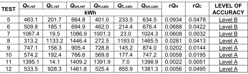
The results of the model simulation for each of the test cases are given in Table 1. The calculated values are compared to the reference values using Eq. (2)-(3)
TEST QH,ref QC,ref Qtot,ref QH,calc QC,calc Qtot,calc rQH rQC ACCURACY LEVEL OF kWh
5 463.1 201.7 664.8 401.0 233.5 634.5 0.0934 0.0478 Level B
6 509.8 185.1 694.9 462.0 214.4 676.4 0.0688 0.0422 Level B
7 1067.4 19.5 1086.9 1001.3 23.0 1024.3 0.0608 0.0032 Level B
8 313.2 1133.2 1446.4 272.5 1193.0 1465.5 0.0281 0.0413 Level A
9 747.1 158.3 905.4 728.8 145.2 874.0 0.0202 0.0144 Level A
10 574.2 192.4 766.6 569.8 177.4 747.2 0.0058 0.0195 Level A
11 1395.1 14.1 1409.2 1391.9 7.0 1398.9 0.0022 0.0051 Level A
[image:3.595.99.500.653.774.2]12 533.5 928.3 1461.8 525.4 855.9 1381.3 0.0056 0.0495 Level A
H H,calc H,ref tot,ref
rQ abs(Q Q ) /Q (2)
C C,calc C,ref tot,ref
rQ abs(Q Q ) /Q . (3) The level of accuracy can be checked with levels: A, B, C. The validation tests are complied with if for each of the cases 5 to 12:
H C
H C
H C
Level A: r 0.05 and r 0.05; Level B: r 0.10 and r 0.10; Level C: r 0.15 and r 0.15.
Q Q
Q Q
Q Q
This relation is used instead of a direct comparison (e.g. QC,calc vs. QC,ref), because a relative difference of, say, 40% in this cooling requirement has no real meaning if the level of cooling required is negligible compared to the energy need for heating.
As can be seen from the results in Table 1, the model shows a high level of accuracy across all the validation tests, with Level A being reached for five out of eight cases. Additionally, the test cases in which greater accuracy is achieved are the tests when the adiabatic ceiling is replaced with a roof with heat transfer to the outside environment.
With a baseline validated model comprised of only five ODEs in state-space form, a malleable framework is provided in which the equations can be modified in order to implement different serving systems into the building model. This also delivers a model that can be used in state-space controller design procedures.
CHP and thermal energy storage models Extending the validated building model, the equations can be modified to include the CHP plant and the thermal energy store. The CHP is represented by a simplified energy-based model given by Eq. (4)
CHP fH gas( )t
, (4)
where εis the efficiency of the CHP plant, fH is the fraction of fuel power converted to thermal power, and ϕgas is the controllable input of fuel into the engine. It follows that the electrical power produced by the CHP engine will be given by Eq. (5)
CHP( ) (1 H) gas( )
P t f t . (5) The thermal energy store model also uses an energy-based approach and is given by Eq. (6)
0
store( ) CF store( ) store( )0 t
t
Q t f
t d t , (6)where ϕstore(t) is the amount of thermal power extracted from or supplied to the store at the current time-step and dϕstore(t0) is the previous value of the integration. This is required as the state of charge (SOC) of the thermal energy store is required by the controller.
With these equations the thermal power supplied to the air node, ϕH, in Eq. (A1) can be replaced with:
H( )t fH gas( )t store( )t
(7)
Both the CHP and thermal energy store have physical limitations that must be modelled to ensure they more closely resemble reality. The CHP engine will have a maximum fuel supply denoted by ϕCHP,max. The CHP engine modelled in this case is based upon a Free Piston Stirling Engine [14], which generates 6 kW of heat and 1 kW of electricity by driving a magnetic piston up and down within a generator coil. The unit can also modulate down to as low as 3 kW, while still generating electricity.
The physical limits of the thermal store are numerous and the following are accounted for in the model. The maximum amount of heat it is able to absorb is equal to the amount of thermal energy being produced by the CHP engine, given by –εfHϕgas(t), since it cannot extract heat from the zone. Additionally, the thermal store has a thermal energy capacity, Qcap., where the correct sizing for the building zone modelled is determined using an iterative procedure given in the subsequent Results section.
Control strategy
The dynamic model of the building and its servicing systems are modelled in the time-domain using a state-space representation of the differential equations1 given by
( ) ( ) ( ) ( ) ( ) ( )
( ) ( ) ( ) ( )
t t t t t t
t t t t
x A x B u M w
y C x D u N w
, (8)
where x(t) is the state vector, defined as the
nodal temperatures T
a iw r f s
( ) [t T T T T T ]
x , u(t)
is the input vector, defined as T gas store
( ) [t ]
u ,
and w(t) is the disturbance input vector, defined as w( ) [t T Io sol Iint Ppv].
Equation (8b) is the algebraic output equation from which all other system variables can be found. In this system there are two outputs: the controlled temperature and the electrical grid power. The controlled temperature in this case is purely the air temperature of the zone i.e.
1( ) a( )
y t T t (9) The electrical grid power is given by
2( ) grid( ) int( ) pv( ) chp( )
y t P t P t P t P t
2( ) int( ) pv( ) (1 H) gas( ).
y t P t P t f t (10)
The state-space matrices (A, B, C, D, M, and N) for the system can be found by substituting Eq. (A1)-(A5), (9) and (10) into the state-space representation given in Eq. (8). These are provided in the Appendix.
[image:5.595.308.527.67.344.2]The control strategy employed uses nonlinear inverse dynamics controller design methods [15] originally used in the aerospace and robotics industry, and more recently applied to the controllability of buildings [7]. Known as RIDE (Robust Inverse Dynamics & Estimation), this time-domain method, expressed in terms of state variables, is used to design a suitable compensation scheme for the control system.
Figure 2. RIDE control system schematic
As shown in Figure 2, the RIDE methodology is comprised of two control signals: Uc which is a function of the error between the reference set-point and the relative output; and Utrim, which is based upon full-state feedback of the system’s current state and disturbance inputs. This allows the RIDE controller to compensate for the disturbance inputs and slow building dynamics. This implementation of the RIDE control algorithm is based upon an ‘ideal control philosophy’ which aims to show that for a given design, if ideal control is feasible while maintaining the stability of the system. However, it has been shown that by rapid estimation of the Utrim term, the RIDE control design methodology can be implemented in practice [15].
The control signal (in the Laplace domain) is given by
trim
( )s C( )s ( )s
U U U , (11)
where
( ) ( ) ( )
C s s s
U K Σ E (12)
trim( )s ( )s ( ) (s s ) ( )s
U K CAX N CM W , (13)
and the controller matrix K( )s (sD CB )1. The overall control strategy alternates between two RIDE control modes: the default, for when the thermal store has spare capacity, and another for when it is saturated (i.e. 100% capacity). The controller signals are found by substituting the state-space matrices into Eq. (11)–(13). Taking the inverse Laplace transform and simplifying, the control signals for the default mode are given by
max
0 min
2 2 0
gas
0 H
pv int
(1/ ) ( ) ( ) 1
( )
(1 )
( ( ) ( ))
t
t
e t t dt t
f
P t P t
(14)
max
H gas
store,H store,P ( )
( ) ( ) ( )
store
f t
t t t
(15)
where
a
store,H 1 iw a iw
1
r a r f a f
s a s
v ni g a o
sa gl g sol int,c f int
( ) ( ) ( ( ) ( ))
( ( ) ( )) ( ( ) ( ))
( ( ) ( ))
( ( ) )( ( ) ( ))
( ) ( ) ( )
C
t e t H T t T t
H T t T t H T t T t H T t T t
H t H H T t T t f g A I t f A I t
(16)
0
2 2 0
H store,P
0 H
pv int
(1/ ) ( ) ( ) ( )
1
( ( ) ( ))
t
t
e t t dt f
t f
P t P t
. (17)
When the store is full, it can no longer absorb the excess heat generated by the CHP to fulfil the electrical energy demand. Therefore, when the store is saturated, the control is switched to mode 2, where: gas( )t store,P( ) 0t . The
[image:5.595.70.289.244.345.2]control mode switching is determined using the combinatorial logic table given in Table 2.
Table 2. Control mode combinatorial logic table
LOGICAL TESTS
MODE store( ) cap.
Q t Q Qstore( )t f Qcyc. cap. Memory
FALSE FALSE Default Default
FALSE FALSE Mode 2 Mode 2
FALSE TRUE Default Default
FALSE TRUE Mode 2 Default
TRUE FALSE Default Mode 2
TRUE FALSE Mode 2 Mode 2
TRUE TRUE Default Default
TRUE TRUE Mode 2 Default
In control mode 2, the store fulfils the heat demand, while the electrical demand will be met by the grid. The control logic contains a thermal energy store ‘cycle capacity’, which stops rapid mode switching around the maximum capacity of the store. The specific cycle capacity can be set on a case by case basis, but results have shown improved energy performance at low (10-20% of maximum capacity) cycle capacities. Controllability
key component of both UC and Utrim. Therefore, in order to ensure that the system can be controlled via the RIDE methodology, it is critical that (sD+CB) is invertible. This is done by ensuring that the determinant is not equal to zero i.e.
0
sD CB . (18)
The matrices B, C, and D are substituted into Eq. (18) and simplified to produce:
H
(1 f ) /Ca 0
(19)
Consequently, the following conditions exist for controllability:
The CHP is operational (ε 0)
A fraction of the gas input into the CHP engine is converted to electricity (fH 1) Therefore, as long as the CHP engine is operational, and it simultaneously produces electricity and thermal energy, then the system will be controllable.
RESULTS AND DISCUSSION
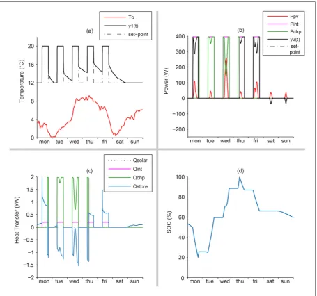
Simulation ParametersThe results given here are calculated using two reference set-points. The first is the controlled temperature (in this case the air temperature of the zone). This heating set-point is 20°C between 08:00 and 18:00 on weekdays, with a night-time and weekend setback temperature of 12°C. The second is the national grid power set-point, which is set to zero. This means that the controller will strive to neither import or export from or to the national grid, thereby minimising the use of the grid.
[image:6.595.71.527.320.746.2]The building zone modelled is Test 9 from the model validation section, and retains the same climate data as before. The internal gains are defined per floor area at 20W/m2 and are defined as 50% convective to the internal air of the zone and 50% radiative to the walls and floor. These internal gains also constitute the
electrical demands of the zone.
The energy production from photovoltaics is calculated using PVWatts [16]. The PV system characteristics consist of a 650W solar array, south facing with a fixed tilt of 48.73° (which is equal to the latitude of the climate data). In all simulations there was a total available power from photovoltaics amounting to 538 kWh over the year.
Simulation Results
Figure 3 shows the dynamic results from the model over the period of a week in November. Table 3 shows the gas and electrical grid utilisation for the year for the model in comparison with several alternative systems.
Table 3. Energy and CO2 emissions comparison SYSTEM Qgas Egrid 1 CO2 (kg)
Condensing Boiler 983.5 672.7 532.2
Air Source Heat Pump N/A 931.5 484.7
CHP & Thermal Store 1201.7 492.4 478.8
1 E
grid is the total electrical energy imported from the grid: for heating, lighting, and appliances
The results for the condensing boiler system are based upon a high efficiency grade A unit with a seasonal efficiency of 91.1%. The air source heat pump (ASHP) results are calculated using the methodology given in [17]. The CO2 emissions for each system are calculated using the latest emission factors from Defra (updated 31st May 2012).
The results show that the CHP & Thermal Store model effectively reduces the use of the national grid and consequently reduces the CO2 emissions over the other systems.
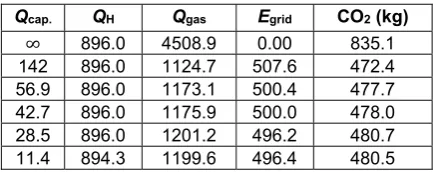
[image:7.595.70.287.676.762.2]The model can be used to size the thermal energy store for the particular building zone modelled by using an iterative design procedure. The model begins with an infinite thermal energy capacity in order to determine the heat and electrical demands of the building zone over a simulated year. It then reduces the size of the thermal store incrementally until the heating set-point cannot be met, indicating the store does not have a sufficient thermal energy capacity. Table 4 highlights the influence of the size of the store on the energy performance of the building zone.
Table 4. Thermal store sizing results
Qcap. QH Qgas Egrid CO2 (kg)
∞ 896.0 4508.9 0.00 835.1
142 896.0 1124.7 507.6 472.4
56.9 896.0 1173.1 500.4 477.7
42.7 896.0 1175.9 500.0 478.0
28.5 896.0 1201.2 496.2 480.7
11.4 894.3 1199.6 496.4 480.5
Results indicate that the 11.4 kWh thermal energy store, which for a wet system would approximate to a 200L water storage tank, is undersized for this building zone. This is because it is unable to deliver the required thermal energy over the year, 896.0 kWh, which is calculated using the infinite thermal energy store.
The results also show that generally, the larger the thermal store the lower the overall energy consumption and CO2 emissions. However, with an idealised infinite thermal store, the total energy supplied and resultant CO2 emissions are higher than the stores with a fixed thermal capacity. This is because the controller will always use the CHP to meet both the thermal and electrical demands over the year, and dumps the excess thermal energy produced into the store which is never fed back into the system.
CONCLUSION AND FUTURE WORK
A simplified dynamic building physics model with energy performance results validated with EN 15265 has been presented. The validity of the modelling approach taken has been highlighted in this paper. This research confirms that it is possible to run an electrically led CHP system, with a coupled thermally/electrically led thermal energy store. Modifications were made to the building model to allow for the simplified implementation of energy based models for a CHP plant and thermal energy store. The flexibility of this modelling approach is highlighted by the simplicity of adding aforementioned systems into the model. It has also been demonstrated that the sizing of the thermal energy store is an optimisation problem that could be expanded on in the future.energy storage to the system could be investigated. This can be used to suggest the energy benefit gained from a building changing its heating system. Energy savings generated by this model can be monetised and used as a basis to suggest the payback period for a building to upgrade its heating system.
The modelling environment could be amended to more closely model real life. For example, state-estimation can be added to the Utrim parameter to determine controller performance that is closer to reality. Additionally, the nonlinearities of the model can be included in the equations themselves in order to assess the controllability under the nonlinear operating conditions which would lead to refinements in the controller design methodology.
The controller presented here is based upon inverse dynamics. Other controllers can be assessed using this model. An interesting area of future work would be to compare the RIDE controller with a more simplistic controller to gauge the benefit of advanced control on a building’s energy use.
Controllable lighting can be taken into account within the model. On average lighting accounts for 32% of the electrical energy use in commercial buildings the UK [19], more than double that of the computing devices (15%). Controllability of lighting is an area of exciting future research: using this modelling approach it can be determined if it is possible to control lighting to help ensure more autonomous behaviour in buildings.
REFERENCES
[1] J. Clarke, C. Johnstone, N. Kelly, P. Strachan, P. Tuohy, The role of built environment energy efficiency in a sustainable UK energy economy, Energy Policy, 36 (2008) 4605-4609.
[2] European Construction Technology Platform, Challenging and changing Europe’s built environment. A vision for a sustainable and competitive construction sector by 2030, in,
Available at
http://www.ectp.org/documentation/ECTP-Vision2030-25Feb2005.pdf, 2005.
[3] Energy Efficiency in Buildings, Transforming the Market: Energy Efficiency in Buildings, in, World Business Council for Sustainable
Development,, Available at
http://www.wbcsd.org/transformingthemarketeeb .aspx, 2009.
[4] P. Tuohy, Davis Langdon LLP, Benchmarking Scottish energy standards: Passive House and CarbonLite Standards: A comparison of space heating energy demand using SAP, SBEM, and PHPP methodologies,
in, The Scottish Government, Available at
http://www.scotland.gov.uk/Resource/Doc/2177 36/0091333.pdf, 2009.
[5] W. Feist, Certified Passive House - Criteria for Non-Residential Passive House Buildings, in, Passive House Institute, Available at
http://passiv.de/downloads/03_certfication_criter ia_nonresidential_en.pdf, 2012.
[6] P.J. Mago, A. Hueffed, L.M. Chamra, Analysis and optimization of the use of CHP-ORC systems for small commercial buildings, Energy and Buildings, 42 (2010) 1491-1498. [7] J. Counsell, Y. Khalid, J. Brindley, Controllability of buildings: A input multi-output stability assessment method for buildings with slow acting heating systems, Simulation Modelling Practice and Theory, 19 (2011) 1185-1200.
[8] British Standards Institution, BS EN 15265: Energy performance of buildings. Calculation of energy needs for space heating and cooling using dynamic methods. General criteria and validation procedures, in, British Standards Institution, London, UK, 2007.
[9] G. Murphy, Y. Khalid, J. Counsell, A simplified dynamic systems approach for the energy rating of dwellings, in: Building Simulation 2011, International Building Performance Simulation Association, Sydney, Australia, 2011.
[10] G. Murphy, J. Counsell, Symbolic energy estimation model with optimum start algorithm implementation, in: CIBSE Technical Symposium 2011, Chartered Institution of Building Services Engineers, Leicester, UK, 2011.
[11] British Standards Institution, BS EN ISO 13786: Thermal performance of building components. Dynamic thermal characteristics. Calculation methods, in, British Standards Institution, London, UK, 2007.
[12] L. Pipes, Matrix analysis of heat transfer problems, Journal of the Franklin Institute, 263 (1957) 195-206.
[13] British Standards Institution, BS EN ISO 6946: Building components and building elements. Thermal resistance and thermal transmittance. Calculation method, in, British Standards Institution, London, UK, 2007.
[14] Baxi, The Baxi Ecogen Dual Energy System, in, Baxi, Available at
http://www.baxiknowhow.co.uk/assets/baxi-ecogen.pdf, 2012.
[16] National Renewable Energy Laboratory, PVWatts, in, U.S. Department of Energy,
Available at
http://rredc.nrel.gov/solar/calculators/PVWATTS/ version1/, 2012.
[17] G. Murphy, J. Counsell, E. Baster, J. Allison, S. Counsell, Symbolic modelling and predictive assessment of air source heat pumps, Building Services Engineering Research & Technology, 34 (2013) 23-39.
[18] R. Hitchin, A guide to the simplified building energy model (SBEM): What it does and how it works, IHS BRE Press, Bracknell, UK, 2010. [19] Department of Energy & Climate Change, Energy Consumption in the UK, Table 5.6a, in: Energy Consumption in the UK, Available at
http://www.decc.gov.uk/en/content/cms/statistics /publications/ecuk/ecuk.aspx, 2012.
NOMENCLATURE
A area, m2
c specific heat capacity, J/(kg·K)
C heat capacity, J/K
d layer thickness, m
E electrical energy, kWh
f fraction/factor
g total solar energy transmittance of element
h surface heat transfer coefficient, W/(m2·K) H heat transfer coefficient, W/K
Iint total heat flux from internal sources, W/m2 Isol solar irradiance, W/m2
P electrical power, W
Q quantity of heat or energy, kWh
R thermal resistance, m2·K/W T thermodynamic temperature, K
U thermal transmittance, W/(m2·K) V volume of air in conditioned zone, m3 Vector-Matrix
A system matrix
B input matrix
C output matrix
D feedforward matrix
E error matrix
K controller matrix
M system disturbance matrix
N output disturbance matrix
R reference input (set-point)
u input or control vector
w disturbance vector
x state vector
x derivative of the state vector w.r.t. time
y output vector
Greek symbols
α absorption coefficient of solar radiation
δ small amplitude perturbation
ε emissivity of surface to long-radiation
κ heat capacity per area, J/(m2·K)
μ integrator output
Σ decoupling matrix
τ time constant, s
ϕ heat flow rate/thermal power, W
Subscripts
a air c convective calc calculated
cap. energy capacity
cyc. thermal store state-of-charge cycle limit C cooling
CF conversion factor, W-kWh f floor
gl glazing H heating int internal
iw internal walls
ni natural infiltration
pv photovoltaic r roof/ceiling rad radiative ref reference s structure sa solar to air sol solar
ss solar to surface of component tot total
int,
, int, int,
df,r ss gl g r r *
df,f ss gl g int,f int,rad f
df,s ss gl g s s int,s int,rad f s* s ( ) 0 0 0 0 0 0 0 0
g ni v sa gl g c f
a a a
ss df iw gl g iw rad iw
iw iw
r r
r r
f f
s s s
H H H t f g A f A
C C C
f f g A f f A
C C
f f g A g A U A
C C
f f g A f f A
C C
f f g A g A f f A U A
C C C
M 1 0 0 0 0 0 0 0 0 H a a f C C B
1 0 0 0 0 0 0 0 0 0
C
H
0 0
(1 f ) 0
D
APPENDIX
Set of five ordinary differential equations that comprise the building model:
HC
sa gl g int,c f int
( )
(1/ )( ( ) ) ( ) (1/ ) ( ) (1/ ) ( )
(1/ ) ( ) (1/ ) ( ) (1/ ) ( ) (1/ )( ( )) ( )
(1/ ) ( ) (1/ ) ( )
a
a g ni v iw r f s a a iw iw a r r
a f f a s s a a g ni v o
a sol a
dT t
C H H H t H H H H T t C H T t C H T t dt
C H T t C H T t C t C H H H t T t C f g A I t C f A I t
(A1) iw
iw iw a iw iw rad,iw-r rad,iw-f rad,iw-s iw rad,iw-r r
iw rad,iw-f f iw rad,iw-s s iw df,iw gl g sol iw int,iw int,rad f int
( )
(1/ ) ( ) (1/ )( ) ( ) (1/ ) ( )
(1/ ) ( ) (1/ ) ( ) (1/ ) ( ) (1/ ) (
iw
ss
dT t
C H T t C H H H H T t C H T t
dt
C H T t C H T t C f f g A I t C f f A I t
)
(A2)
r
r r a r rad,iw-r iw r r r* r rad,iw-r rad,r-f rad,r-s r
r rad,r-f f r rad,r-s s r r* r o r df,r ss gl g r r sol
( )
(1/ ) ( ) (1/ ) ( ) (1/ )( ) ( )
(1/ ) ( ) (1/ ) ( ) (1/ ) ( ) (1/ )( ) ( )
dT t
C H T t C H T t C H U A H H H T t
dt
C H T t C H T t C U AT t C f f g A g A I t
(A3)
f
f f a f rad,iw-f iw f f rad,iw-f rad,r-f rad,f-s f
f rad,r-f r f rad,f-s s f df,f ss gl g sol f int,f int,rad f int
( )
(1/ ) ( ) (1/ ) ( ) (1/ )( ) ( )
(1/ ) ( ) (1/ ) ( ) (1/ )( ) ( ) (1/ )( ) ( )
dT t
C H T t C H T t C H H H H T t
dt
C H T t C H T t C f f g A I t C f f A I t
(A4)
s
s s a s rad,iw-s iw s rad,r-s r s rad,f-s f
s s s* s rad,iw-s rad,r-s rad,f-s s s s* s o
s df,s ss gl g s s sol s int,s
( )
(1/ ) ( ) (1/ ) ( ) (1/ ) ( ) (1/ ) ( )
(1/ )( ) ( ) (1/ ) ( )
(1/ )( ) ( ) (1/ )(
dT t
C H T t C H T t C H T t C H T t dt
C H U A H H H T t C U A T t
C f f g A g A I t C f f
int,radA I tf) ( )int
(A5)
State-space matrices
iw rad,iw-r rad,iw-f rad,iw-s ,
1
,
2
( ( ) )
(1/ ) 0 0 0 0
( )
0 (1/ ) 0 0 0
0 0 (1/ ) 0 0
0 0 0 (1/ ) 0
0 0 0 0 (1/ )
(1/ ) 0 0 0 0
0
g ni v iw r f s iw
a
iw iw
r
r rad iw r
f f rad iw f
s s iw
a
H H H t H H H H H
C
H H H H H
C
H H
C
C H H
C H H
C A A , ,
r r* r rad,iw-r rad,r-f rad,r-s ,
, f rad,iw-f rad,r-f rad,f-s
, ,
(1/ ) 0 0 0
( )
0 0 (1/ ) 0 0
0 0 0 (1/ ) 0
0 0 0 0 (1/ )
r f
rad iw r rad iw f
iw
rad r f r
f rad r f
s rad r s rad f s
H H
H H
C
H U A H H H H
C
C H H H H H
C H H
A , , 3 ,
s s* s rad,iw-s rad,r-s rad,f-s
(1/ ) 0 0 0 0
0 (1/ ) 0 0 0
where
0 0 (1/ ) 0 0
0 0 0 (1/ ) 0
0 0 0 0 (1/ ) ( )
s a
rad iw s iw
rad r s r
f rad f s
s H C H C H C C H
C H U A H H H
1 2 3 A A A A
f 0 0 0 0 0 0 A 1