Longitudinal and transverse cooling of relativistic electron beams in intense laser pulses

This content has been downloaded from IOPscience. Please scroll down to see the full text.

Download details:

IP Address: 130.159.82.28

This content was downloaded on 18/05/2015 at 13:24

Please note that terms and conditions apply.

Longitudinal and transverse cooling of relativistic electron beams in intense laser pulses

View the table of contents for this issue, or go to the journal homepage for more 2015 New J. Phys. 17 053025

PAPER

Longitudinal and transverse cooling of relativistic electron beams in

intense laser pulses

Samuel R Yoffe1

, Yevgen Kravets1,2

, Adam Noble1

and Dino A Jaroszynski1

1 _{Department of Physics, SUPA, University of Strathclyde, Glasgow G4 0NG, UK} 2 _{Centre de Physique Théorique, École Polytechnique, F-91120 Palaiseau, France} E-mail:adam.noble@strath.ac.ukandd.a.jaroszynski@strath.ac.uk

Keywords:electromagnetism, radiation reaction, quantum effects

Abstract

With the emergence in the next few years of a new breed of high power laser facilities, it is

becoming increasingly important to understand how interacting with intense laser pulses affects

the bulk properties of a relativistic electron beam. A detailed analysis of the radiative cooling of

electrons indicates that, classically, equal contributions to the phase space contraction occur in

the transverse and longitudinal directions. In the weakly quantum regime, in addition to an

overall reduction in beam cooling, this symmetry is broken, leading to signi

fi

cantly less cooling in

the longitudinal than the transverse directions. By introducing an ef

fi

cient new technique for

studying the evolution of a particle distribution, we demonstrate the quantum reduction in beam

cooling, and

fi

nd that it depends on the distribution of energy in the laser pulse, rather than just

the total energy as in the classical case.

1. Introduction

The emergence over the next few years of a new generation of ultra-high power laser facilities, spearheaded by the extreme light infrastructure (ELI) [1], represents a major advance in the possibilities afforded by laser technology. In addition to important practical applications, these facilities will, for thefirst time, allow investigation of qualitatively new physical regimes. Among thefirst effects to be explored will be radiation reaction.

Radiation reaction—the recoil force on an electron due to its emission of radiation—remains a contentious area of physics after more than a century of investigation. The standard equation describing radiation reaction (the so-called LAD equation, after its progenitors Lorentz, Abraham, and Dirac [2–4]) for a particle of massm

and chargeqin an electromagneticfieldFreads

τΔ τ

= + ⃛ = − +

(

⃛ −

)

x f

m x

q

mF x x x x x

¨a ˙ ¨ ¨ ˙ , (1)

a a

b b ab b a b b a

ext

wherefa = −qF xa ˙

b b

ext is the Lorentz force. Here, the constantτ≔q 6πm

2 _{is the‘characteristic time’of the}

particle3and an overdot denotes differentiation with respect to proper time. Indices are raised and lowered with the metric tensorη=diag( 1, 1, 1, 1)− , and repeated indices are summed from 0 to 3. Thex˙-orthogonal projectionΔa ≔δ +x x˙ ˙

b ba a bensures thatx¨is orthogonal tox˙, preserving the normalization condition

= − x x˙ ˙a 1

a (equivalently the mass shell condition,p pa a = −m2, wherepa =mx˙a=(γm, )p ). We work in Heaviside–Lorentz units withc= 1.

OPEN ACCESS

RECEIVED

12 March 2015

ACCEPTED FOR PUBLICATION

9 April 2015

PUBLISHED

18 May 2015

Content from this work may be used under the terms of theCreative Commons Attribution 3.0 licence.

Any further distribution of this work must maintain attribution to the author(s) and the title of the work, journal citation and DOI.

3

The characteristic timeτ=2 3r ccan be interpreted as the time taken for light to travel across the classical radius of the particle, πϵ

=

r q24 mc

0 2. For an electron,τe=6.3×10−24s, corresponding tore=2.8×10−15m. Since radiation damping is proportional

to_τ, radiation reaction effects will typically be more prominent for electrons, for whichq= −eandm=me, than for particles with

larger mass.

Equation (1) may be unpacked and expressed in terms of the three-momentum as

γ τγ γ γ

γ

= + × + + −

t q m t t t m t

p

E p B p p p p

d d 1 d d d d d d d

d , (2)

2 2 2 ⎛ ⎝ ⎜ ⎞_⎠⎟ ⎡ ⎣ ⎢ ⎢ ⎛ ⎝ ⎜ ⎞ ⎠ ⎟ ⎛_⎝⎜ ⎞_⎠⎟ ⎛ ⎝ ⎜ ⎞ ⎠ ⎟⎤ ⎦ ⎥ ⎥

whereγ= 1+p2m2_{andd dγ t =( · d d )p p t γm}2_.

Despite numerous independent derivations of equation (1), either on the basis of energy–momentum conservation [4,5] or as the Lorentz force due to the particle’s (regularized) self-field [6], it is subject to numerous difficulties; see the recent review [7] for an account of these problems and proposed solutions. The most widely used alternative to LAD is that introduced by Landau and Lifshitz [8], by treating the self-force as a small perturbation about the applied force and retaining terms to leading order in the small parameterτ:

τ Δ

= − − ∂ −

x q mF x

q

m F x x q

m F F x

¨a ab˙ ˙ ˙ ˙ . (3)

b ⎜⎛_⎝ c ab b c ab bc cd d⎟⎞_⎠

It is often claimed that (3) is valid provided only that quantum effects can be ignored, and though a rigorous demonstration remains elusive there is mounting evidence that this is indeed the case [9,10]. Note that equation (3) can also be presented in terms of the electric and magneticfields,EandB, as [8,11]

γ

τγ

γ γ γ

γ γ γ

= + ×

+ + × + × + × ×

+ + − + ×

t q m

q

t m t

q m m q m q m q m m p

E p B

E p B

E B p B B

p E E p E p E p B p

d d d d d d

( · ) ( · ) , (4)

2 2 2 4

2 2 2 ⎪ ⎪ ⎪ ⎪ ⎛ ⎝ ⎜ ⎞_⎠⎟ ⎧ ⎨ ⎩ ⎛ ⎝ ⎜ ⎞_⎠⎟ ⎡ ⎣ ⎢ ⎛ ⎝ ⎜ ⎞_⎠⎟ ⎤ ⎦ ⎥ ⎛ ⎝ ⎜ ⎞ ⎠ ⎟ ⎫⎬ ⎭

where the total time derivative acting on theE B, fields isd dt = ∂ ∂ +t (1γm) ·p .

Under the conditions expected at ELI, the caveat‘provided that quantum effects can be ignored’is pertinent. Quantum effects are typically negligible if the electricfield observed by the particle,Eˆ, is much less than the Sauter–Schwingerfield [12,13] typical of QED processes, that is provided

χ≔ e = ≪

m F F x x E E

˙ ˙ ˆ 1, (5)

e ab

ac b c S 2

whereES=m c ee2 3 = 1.32×1018V m−

1

is the Sauter–Schwinger criticalfield. For 1 GeV electrons in a laser pulse of intensity 1022W cm−2(parameters obtainable at ELI),χ∼ 0.8and quantum effects cannot be ignored. A complete QED treatment of radiation reaction is difficult to implement and problematic even to define but, providedχremains small, a semi-classical modification to (3) should be valid [14].

An important difference between the classical and quantum pictures of radiation emission can be seen in the radiation spectrum. Classically, a charged particle can radiate arbitrarily small amounts of energy at all

frequencies. However, in the quantum picture, the particle must radiate entire quanta of energy in the form of photons. Thus, the energy (frequency) of the emitted photons is limited by the energy of the particle. This suppresses emission at high frequencies, and introduces a cut-off in the spectral range of the emitted radiation [14]. As such, it is expected that the effects of radiation reaction are overestimated by classical theories in regimes where quantum effects become important [15], since they consider the particle to be radiating at all frequencies.

In order to account for this reduction in the effects of radiation reaction relative to the Landau–Lifshitz equation of motion, we follow Kirket al[16] and scale the radiation reaction force by the functiong( )χ:

χ τ Δ

= − − ∂ −

x q

mF x g q

m F x x q

m F F x

¨a ab˙ ( ) ˙ ˙ ˙ . (6)

b ⎜⎛_⎝ c ab b c ab bc cd d⎟⎞_⎠

The full expression forg( )χ involves a non-trivial integral over Bessel functions. To make this tractable, we use an approximation introduced by Thomaset al[17],

χ =

(

+ χ+ χ + χ

)

−

g( ) 1 12 31 2 3.7 3 4 9. (7)

It can be clearly seen that, in the classical limitχ→0, we haveg( )χ →1, recovering the classical equation of motion (3). As we move into a more strongly quantum regime, the quantum nonlinearity parameterχincreases and the scaling functiong( )χ decreases, in turn reducing the effects of radiation reaction. The model essentially reduces to a rescaling of the characteristic time of the particle,τ→g( )χ τ, which can also be applied to

equation (4). For χ∼ 1, the stochasticity of quantum emission becomes important, and the semi-classical model is no longer applicable [18]. At this point,g( )χ ≃0.18, which corresponds to a significant reduction in

It is generally accepted that radiation reaction effects will be more readily observed in the behaviour of particles than in the radiation they emit [17,19]. As such, it is important to be able to accurately determine the distribution of a bunch of particles evolving according to (3) or its semi-classical extension (6). Usually this would involve solving a Vlasov equation [20] or following the evolution of very large numbers of particles [21], either of which is computationally very intensive.

In this paper we investigate beam cooling of a particle bunch due to classical and semi-classical models of radiation reaction. In section2we present a detailed discussion of longitudinal and transverse phase space contraction of the particle distribution, along with an analytical solution of the classical Vlasov equation. The longitudinal particle distribution is introduced. Since the semi-classical Vlasov equation has no analytical solution, in section3we introduce a new method of accurately reconstructing the particle distribution from the trajectories of a relatively small number of particles. Classical predictions using this method are compared to the analytical solution with excellent agreement. The method is then applied in section4in order to compare classical and semi-classical predictions for an electron beam colliding with an intense laser pulse. Finally, we conclude by summarizing ourfindings in section5.

2. Particle distribution and phase space contraction

The evolution of a particle beam can be described by the Vlasov equation for the particle distributionℱ( , )x u, whereua=( , )γ u _{is the four-velocity. Position and velocity are considered as independent phase space}

variables. The Vlasov equation forℱcan be expressed as

β ℱ = ℱ + ℱ =

s s

d

d ( )

d

d s 0, (8)

⎡ ⎣⎢

⎤ ⎦⎥

whereis the phase-space volume element andβ_s( , )x u describes the rate of change (i.e. expansion or contraction) ofwith proper times. (Technically,β_sis the phase-space divergence of the vectorfield



= ∂ ∂ + ∂ ∂

X ua xa I uI_{(whereis the acceleration) associated with theflowd ds, given by the Lie derivative}

X= βs, see [20].) Capital Latin indices take three values. Unlike the Liouville equation (or the case with no

radiation reaction) the phase-space volume element is not preserved by theflow,β_s≠ 0.

To facilitate investigation of the interaction of a particle bunch with a laser pulse, we introduce the (null) wavevectorksuch that the phase of the pulse is

ϕ= −k x· =ωt−k x· . (9)

The orthogonal (transverse) vectorsϵ λ, satisfying

ϵ2=λ2=1 and k·ϵ=k·λ=ϵ·λ=0, (10)

together withkand the null vectorℓ(defined to satisfyℓ·ϵ=ℓ·λ=0andk·ℓ= −1) form a basis. In addition, the coordinates

ξ=ϵ· ,x σ=λ·x and ψ= −ℓ·x (11)

are also defined, along with the corresponding velocitiesuϕ,uξ,uσanduψ. However,uψis not independent and

may be found from the normalization conditionu ua a=uξ2+uσ2− 2u uϕ ψ = −1. We note that Greek

subscripts are used only as labels and are not free indices.

For a plane wave with arbitrary polarization, the electromagneticfield tensorFdepends on spacetime only through the phaseϕ, and takes the form

ϕ ϵ ϵ ϕ λ λ

= ϵ

(

−

)

+ λ

(

−

)

q

mF a ( ) k k a ( ) k k , (12)

a

b a b a b a b a b

where the functionsaϵ λ, ( )ϕ are dimensionless measures of the electricfield strength in theϵ,λdirection. The

corresponding electric and magneticfields areE=(mω q a)[ ( ) ˆϵ ϕ ϵ+ aλ( ) ˆ]ϕ λ andB=k×E ω, where the

orthogonal unit three-vectorsϵ λˆ, ˆsatisfyk· ˆϵ=k· ˆλ =0.

In a similar manner, we assume that the particle distribution also depends on spacetime only through the phaseϕ, such thatℱ( , )x u = ℱ( ,ϕ uϕ,uξ,uσ). The Vlasov equation is then written

 

ϕ _{  }

∂ℱ ∂ +

∂ℱ ∂ +

∂

∂ ℱ =

ϕ ϕ

ϕ

β

ℱ u

u u u u 0, (13)

I I

s

I I

d d

s

⎛ ⎝ ⎜⎜ ⎞_⎠⎟⎟

whereuI ∈ {uϕ,uξ,uσ}, and the accelerationsI ∈{  ϕ, ξ, σ}follow from the single-particle equations



ϕ β β

ℱ

+ ℱ = = ∂

∂u uϕ d

d 0, where I . (14)

I ⎛ ⎝ ⎜⎜ ⎞_⎠⎟⎟

The quantityβis responsible for any phase space contraction (β<0) or expansion (β>0) of the particle distribution, and the associated change in electron entropy [22].

For a highly relativistic particle beam colliding with a laser pulse (the scenario in which radiation reaction effects are most prominent), we are mainly interested in the dependence ofℱonϕanduϕ. An advantage of the

coordinate system (9)–(11) is that it decouples the longitudinal from the transverse velocity in the Lorentz invariant measure,d ˙3x γ=duξduσdu uϕ ϕ. Hence we can define thelongitudinal distribution

∫

ϕ ϕ = ℱ ξ σ



(

)

f ,u du du , (15)

2

which satisfies thereduced Vlasov equation



ϕ +β = β =

∂ ∂ ϕ ϕ ϕ ∥ ∥ f f u u d

d 0, where . (16)

⎛ ⎝ ⎜⎜ ⎞_⎠⎟⎟

Here,β_∥describes thelongitudinalphase space contraction. The transverse contribution is then

 

β =β−β = ∂

∂ + ∂ ∂ ξ ξ ϕ σ σ ϕ ⊥ ∥

u u u u . (17)

⎛ ⎝

⎜⎜ ⎞_⎠⎟⎟ ⎛_⎝⎜⎜ ⎞_⎠⎟⎟

Note that this reduction to the longitudinal distribution is purely a consequence of the coordinate system, and does not rely on the plane wave assumption.

It is at this point that a decision must be made as to the appropriate single-particle equations of motion. While there are many classical models for radiation reaction [7], we start by considering the Landau–Lifshitz equation given by (3), before moving on to the semi-classical extension (6). This is in part motivated by the existence of an analytical solution to the single-particle Landau–Lifshitz equation [23]. In our coordinates, the Landau–Lifshitz equations in the plane wave (12) are

   τ τ τ τ τ = − = − + ′ − = − + ′ − ϕ ϕ

ξ ϕ ϵ ϕ ϵ ϕ ξ

σ ϕ λ ϕ λ ϕ σ

(

)

(

)

a u

u a u a a u u u a u a a u u

ˆ _,

ˆ _,

ˆ _{, (18)}

2 3

2 2

2 2

wherea2( )ϕ = aϵ2( )ϕ +aλ2( )ϕ and prime denotes differentiation with respect toϕ. Inserting these equations

into (16) and (17), wefind for the classical case

βˆ∥=βˆ⊥= −2τa u2 ϕ⩽0. (19)

It is immediately apparent that half the contraction of the distribution occurs in the longitudinal and half in the transverse directions.

The semi-classical equations of motion are just (18) with the replacementτ→g( )χ τ. However, since

χ ϕ( ,uϕ)=3τa( )ϕ uϕ 2α(whereαis thefine structure constant) depends onuϕ(but not on the transverse

velocities) we pick up an additional contribution to the longitudinal phase space contraction:

 

β= β+ ∂ β β

∂ = + ∂ ∂ ϕ ϕ ϕ ϕ ϕ ϕ ∥ ∥ g g

u u g

g u u

ˆ ˆ _and ˆ ˆ _{; (20)}

whereas, the transverse contraction is simply scaled byg( )χ :

β_⊥=β−β_∥=g

(

βˆ−βˆ_∥

)

=gβˆ_⊥=gβˆ ._∥ (21)

Thus, as quantum effects become more important andg( )χ decreases, the semi-classical model predicts a reduction in both the longitudinal and transverse phase space contraction (reduced beam cooling). As well as this scaling of the classical contraction byg( )χ, there is an additionallongitudinal heatinggiven by

 

χ χ

β χ χ χ χ

∂ ∂ = ∂ ∂ = − + + ⩾ ϕ ϕ ϕ ϕ ϕ ϕ ⊥

(

)

g u u g

u u g

ˆ _d

d

ˆ ₂

9 ( ) 12 62 11.1 0, (22)

9 4 2

⎡

⎣⎢ ⎤⎦⎥

whereβ⊥= gβˆ⊥= −2τa2( ) ( )ϕ g χ uϕ= −4αa( )ϕ χg( ) 3χ . The ratio β

β = − χ χ + χ+ χ ⩽

∥

⊥

(

)

g

1 2

9 ( ) 12 62 11.1 1 (23)

measures the strength of the longitudinal compared to the transverse phase space contraction. This is shown in figure1(a) for the intervalχ∈[0, 1]. Even for the weakly quantum regime in which the semi-classical model remains valid, we observe a significant reduction in longitudinal beam cooling. This is especially clear when comparison is made with the classical resultβˆ_∥as shown infigure1(b). We see that where χ=0.2there is nearly a 60% reduction in the longitudinal contraction experienced compared to the Landau–Lifshitz model.

For the case of the classical Landau–Lifshitz theory in a plane wave, the Vlasov equation (14) may be solved analytically for the particle distribution:

ϕ ϕ

ℱ

(

,uϕ,uξ,uσ

)

= ℱ

(

0,uϕ0,uξ0,uσ0

)

e4Λ ϕ

(

,uϕ

)

, (24)

where

{

ϕ0,uϕ0,uξ0,uσ0

}

are theinitialphase and velocities of a particle with{uϕ,uξ,uσ}at phaseϕ. In a similar

manner, the longitudinal distribution is found to be

ϕ ϕ =

(

ϕ ϕ

)

Λ ϕ ϕ

(

)

(

)

f ,u f 0,u0 e2 ,u . (25)

The contraction/expansion of phase space is contained in the function

∫

Λ ϕ ϕ =τ ϑ ϑ ϑ

ϕ ϕ

ϕ

(

,u

)

d a2( )u ( ). (26)

0

Solutions to equation (18) [23] can then be used to rewrite

{

ϕ0,uϕ0,uξ0,uσ0

}

in terms of the independent

variables{ ,ϕ uϕ,uξ,uσ}:

 

 



 

τ ϕ

τ ϕ ϕ ϕ

τ ϕ ϕ

τ ϕ ϕ ϕ

τ ϕ ϕ

= −

=

− + −

− −

=

− + −

− −

ϕ

ϕ

ϕ

ξ

ξ ϕ ϵ ϵ ϵ

ϕ

ϵ

σ

σ ϕ λ λ λ

ϕ

λ

(

)

(

)

u u

u

u u u a a

u

u u u a a

u

1 ( ),

( ) ( ) _{( )}

1 ( ) ( ),

( ) ( ) _{( )}

1 ( ) ( ), (27)

0

0

0

0

0

where the functions

 

 

∫

∫

∫

ϕ ϑ ϑ

ϕ ϑ ϑ

ϕ ϑ ϑ ϑ

=

=

=

ϕ ϕ

ϕ ϕ

ϕ ϕ

a

a

a

( ) d ( ),

( ) d ( ),

( ) d ( ) ( ), (28)

i i

i i

2

0

0

0

[image:6.595.120.557.63.206.2]

withi∈ { , }ϵ λ depend only on the properties of the laser pulse.

Using equations (27) we can expressuϕ( )ϑ in equation (26) in terms of the independent variableuϕ,

  

∫

Λ ϕ τ ϑ ϑ

τ ϕ ϑ

τ ϕ = − − = − − ϕ ϕ ϕ ϕ ϕ ϕ

(

)

(

u

)

u a

u u

, d ( )

1 ( ( ) ( ))

ln 1 ( ) , (29)

2

0

such that the distribution becomes

 ϕ ϕ τ ϕ ℱ = ℱ −

ϕ ξ σ

ϕ ξ σ

ϕ

(

)

(

)

(

u u u

)

u u u u

, , , , , ,

1 ( )

, (30)

0 0 0 0

4

or for the longitudinal distribution

   ϕ ϕ τ ϕ ϕ τ ϕ τ ϕ = − = − − ϕ ϕ ϕ ϕ ϕ ϕ

(

)

(

)

(

)

(

)

f u f u

u

f u

u u

, ,

1 ( )

,

1 ( )

1 ( )

. (31) 0 0 2 0 2 ⎛ ⎝ ⎜⎜ ⎞_⎠⎟⎟

This latter result is in agreement with observations made by Neitz and Di Piazza [24], and we see that the longitudinal distribution is only sensitive to the properties of the laser pulse through the function( )ϕ. After the pulse has passed,becomes constant and is proportional to thefluence of the pulse. Final-state properties of the longitudinal distribution therefore depend only on the total energy contained in the laser pulse, and are insensitive to how that energy is distributed within the pulse. The full distributionℱ, on the other hand, depends additionally on the integralsigiven in equation (28).

Although the reduced Vlasov solution (31) is somewhat simpler than (30), and captures the key features of the electron beam itself, the solution is not sufficient to calculate the transverse current density, and hence cannot be coupled to Maxwell’s equations to determine the radiation produced by the electron beam. However, if the transverse momentum spread is sufficiently small, we can approximate the full distribution by

 

ϕ ϕ δ ϕ δ ϕ

ℱ

(

,uϕ,uξ,uσ

)

=f

(

,uϕ

)

(

uξ− ϵ

(

,uϕ

)

) (

uσ − λ

(

,uϕ

)

)

, (32)

where theδ-functions restrict the transverse velocities to the submanifoldi. Then, in addition to (16), equation (14) yields

  _

ϕ τ τ τ ϵ λ

∂ ∂ − ∂ ∂ = − + ′ + ∈ ϕ ϕ ϕ ϕ

(

)

a u

u a u a u a , fori { , }. (33)

i i

i i i

2 2 2

Note that (33) indicate that the distribution is concentrated on a surface in phase space that itself satisfies the

Landau–Lifshitz equation.

Given solutions to the reduced Vlasov equation (31) and the transverse Landau–Lifshitz equation (33), the current can be written

∫

ϱℓ

= ℱ ξ σ = + +

ϕ

ϕ ⊥ ∥

j q x u u u

u j j

˙ d d d , (34)

a a a a a

withj_⊥aandϱevaluated as

 

∫

∫

∫

ϵ λ ϱ

= ϵ + =

ϕ ϕ λ ϕ ϕ ϕ ⊥

j q f u

u q f u

u q f u

d d

and d . (35)

a a a

We could also calculatej_∥adirectly, but it follows more straightforwardly from charge conservation,∂aja =0.

In the following, we restrict our attention to the longitudinal distributionf( ,ϕ uϕ), and longitudinal beam

cooling, as this is more readily measurable in experiments than the transverse cooling. However, the transverse cooling, which can be considerably greater, can be determined from equation (23).

3. Numerical (re)construction of the particle distribution

for a variety of systems, here we consider a distribution of particles subject to equation (3) and its semi-classical extension (6), without particle-particle interactions4.

Assuming that the laser pulse can be approximated by a plane wave with compact longitudinal support5, any spatial spread in the initial particle distribution would only determine the moment when each particular particle enters the pulse. For simplicity, we therefore take all particles to originate from the same point. This is reasonable as we are primarily interested in the longitudinal momentum distribution.

Since our pulse is modelled by a plane wave and we focus on the longitudinal properties of the distribution, we consider the initial momenta to be strongly peaked about zero in the transverse directions. As such, the initial distribution can be taken to be a Maxwellian distribution for the (longitudinal) momentump(in units ofmc)

ϕ

πθ θ

= = − −

f( 0, )p N p p

2 exp

( ¯ )

2 , (36)

P ⎡ 2

⎣

⎢ ⎤

⎦ ⎥

withϕ=ωt−k x· the phase,θthe variance of the distribution, andNPthe number of particles. The momentumpis related to our velocities of section2by

ω γ γ ω

ω

= ϕ − = + + +

ξ σ ϕ

ϕ

(

)

(

)

p u u u u

u

, where 1

2 . (37)

2 2 2

We stress that this initial distribution is chosen for its simplicity; alternative distributions could be used where appropriate (such as Maxwell–Jüttner).

Typically, one would sample the distribution at random, which would require a large number of particles to accurately represent the distribution. Instead, since the particle number is simply

∫

ϕ

= −∞

∞

NP dp f( , ),p (38)

we determine the momentum spacingδpbetween the particles from the initial distribution by truncating the integral in (38) so that the particle number increases by unity in the given momentum interval:

∫

δ

= _δ ≃

− +δ

p f p f p p

1 d (0, ) (0, ) . (39)

p p p

2

p 2

This leads to a set ofNP=2Nc+1initial momentaV(0)=

{

pi(0)

}

fori∈ −[ N Nc, c], with thepigenerated iteratively fromp₀ = p¯andp_±1= p¯ ±1 f(0, ¯)p using

ξ

ξ

= _ξ + =

ξ

−

−

(

)

p p

f p

i

2

0,

with sgn( ). (40)

i i

i 2

The momentum space is not sampled uniformly, instead more particles are located in regions where the distribution function is large.

As the evolution proceeds, this procedure is applied in reverse to reconstruct the distribution. The set of momentaV( )ϕ is ordered such thatp_i+1⩾p_iand used tofindδp_i( )ϕ =

(

p_i+1( )ϕ −p_i−1( ) 2ϕ

)

. The velocity distribution is then defined to be

ϕ

δ ϕ

≔

(

)

f p

p

, 1

( ). (41)

i i

Reconstruction of a distribution from a particle sample can be problematic, but in our formalism it becomes quite natural. This is achieved by using the momentum spacing between particles to determine the value of the distribution such that equation (39) is satisfied for allϕ(i.e. integration over each of the measured momentum spacings always contributes a single particle to the total particle number). The closer the measured momenta are together, the‘more likely’one is to have a particle in that momentum range, resulting in a larger value for the distribution.

The definition (41) allows properties of the distribution to be calculated directly from the momenta of the individual particles. The mean is simply evaluated as

4

For a highly relativistic particle bunch, these interactions can be neglected on the time scale of the laser interaction.

5



∫

∑

∑

ϕ ϕ ϕ

ϕ ϕ δ ϕ

ϕ

= =

≃

=

=

(

)

p p

N p pf p

N p f p p

N p

¯ ( ) ( ) 1 d ( , )

1

( ) , ( )

1

( ). (42)

P

P _i i i i

P _i i

1

In a similar manner, higher-order moments of the distributionXnmay be calculated straightforwardly as:

∑

ϕ = − ϕ ≃ ϕ − ϕ

X p p

N p p

( ) ¯ ( ) 1 ( ) ¯ ( ) . (43)

n

n

P _i i

n

⎡⎣ ⎤⎦ ⎡⎣ ⎤⎦

For example, the varianceθ ϕ( )=X2( )ϕ and skewnessS( )ϕ =X3( )ϕ X23 2( )ϕ. We note that angular brackets

〈⋯〉will be used to denote an average over the bunch, not time.

A major advantage of this new methodology is that the distribution can be accurately represented and reconstructed using far fewer particles than would be required using random sampling. Figure2(a) shows a simple Gaussian distribution with zero mean and unit variance,A z( ) =(1 2 )exp(π −z2 2)_{, reconstructed}

using two methods. First, the distributionA(z) was sampled according to the iterative relation (40) with

=

NP 401and then reconstructed using (41) (—). Next,Nz= 100 000 random numbers were generated from

A(z) using a Mersenne-Twister pseudo-random number generator, from which the distribution was found using 100fixed-width bins(‐ ‐ ‐). Even with 100 000 random samples, the standard approach does not describe the Gaussian perfectly, while the new method presented in this paper does an excellent job using only 401 points. For comparison, a sample ofNz= 401 was also reconstructed using 50fixed-width bins (–·–). The advantage of the new method with such a small sample size is clear.

Figure2(a) also shows how sampling the distribution according to equation (40) cuts off the tails of the distribution, which will have an effect on the measured properties of the reconstructed distribution. Thefinite number of particles used to represent the distribution causes the measured relative momentum spread (defined by equation (44) below) to be less than that specified when defining the initial distribution. Essentially, it comes

down to the‘≃’in equation (39), compared to the definition given by equation (41). AsNPis increased, the approximation in equation (39) improves, and the measured value approaches the desired value. In addition, with more particles the distribution is sampled further into the tails. Figure2(b) shows the measured initial spread,σˆi, as a fraction of the desired spread,σˆd, when the particle number is varied from as few as 11 up to

=

NP 2001. We see that the approximation quickly improves asNPis increased up to about 500. The value

=

NP 401is chosen to give less than 0.5% error in the initial measured momentum spread. In practice, good

[image:9.595.120.554.63.207.2] [image:9.595.251.402.295.392.2]

agreement can be found with lowerNP, with the caveat that properties sensitive to the tails of the distribution (such as the skewness) may be strongly affected. (This is confirmed infigure3, where the distribution and its statistics calculated from the analytical solution to the classical Vlasov equation are compared to those obtained with this new method.)

Figure 2.(a): A Gaussian distributionA(z) is reconstructed using the new method described by equations (40) and (41) with =

NP 401particles (red, solid) and compared to the standard approach of random sampling, using bothNz= 401 (blue, dot–dash) andNz=100 000(black, dashed) particles. (b): Variation of the measurement of the initial relative momentum spreadσˆias the

4. Interaction of a particle bunch with high-

fl

uence laser pulses

The analytical solution to the Vlasov equation including radiation reaction according to the Landau–Lifshitz theory derived in section2predicts that the collision of an energetic electron beam with a high-intensity laser pulse leads to a significant contraction of the particle phase space, resulting in a reduction in the relative momentum spread. Agreement between this analytical solution and numerical results obtained using the approach discussed above is shown below to be excellent. As previously observed, classical beam cooling depends only on the totalfluence of the pulse, rather than its duration or peak intensity independently [24,27]. However, for the semi-classical extension, the Vlasov equation is no longer tractable. This highlights the value of our approach and, to demonstrate the use of our proposed method in such a case, we consider the importance of quantum effects in the interaction of an electron bunch with a high-intensity laser pulse.

To establish the impact of quantum effects on the evolution of the particle distribution subject to radiation reaction, we introduce therelative momentum spreadand themomentum skewness(calculated from the meanp¯

and varianceθ):

σ ϕ θ ϕ

ϕ ϕ

ϕ

θ ϕ

= =

−

p S

p p

ˆ ( ) ( )

¯ ( ) and ( )

¯ ( )

( ) . (44)

3

3 2

⎡⎣ ⎤⎦

The former gives a measure of the beam quality, while the latter indicates how symmetric the distribution is about its mean.

We restrict our attention to a linearly polarizedN-cycle plane wave pulse (12), modulated by asin2-envelope [9], withaλ= 0andaϵ=a( )ϕ , where

ϕ = ϕ πϕ <ϕ<

a( ) a sin( )sin ( L) for 0 L,

0 otherwise, (45)

0 2

⎧ ⎨ ⎩

wherea0is the dimensionless (peak) intensity parameter (the so-called‘normalized vector potential’) and

π

=

[image:10.595.121.553.63.339.2]

L 2 Nis the pulse length6. This pulse shape offers compact support, allowing the particles to begin and end in vacuum. The totalfluence (energy per unit area) of the pulse is proportional to

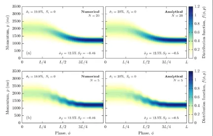
Figure 3.The phase space evolution of the distribution functionf( , )ϕ p predicted by the analytical solution (31) of the reduced Vlasov equation (16), compared to numerical results obtained using the new method presented in section3. Results are presented for (a)N= 20 and (b)N= 5 cycles, whereL=2πNis the pulse length. The_fluence has been kept constant, withNa02=9.248×103.

6

=

_∫

dϕa ( )ϕ = 3πNa

8 . (46)

L 0

2

02

In this work,is kept constant, whichfixesa0for eachN. It has been shown [24,27] (see also section2) that the

classical Landau–Lifshitz prediction for thefinal state of a particle distribution emerging from the pulse is completely determined by thefluence, whereas quantum effects are expected to depend on the value ofa0itself.

We are then able to explore the impact of the reduced emission in the quantum model with varyinga0while

maintaining the same classical prediction. This allows us to explore therelativeimportance of quantum effects. To motivate this study, parameters have been chosen to be relevant at the forthcoming ELI facility. We have chosen to considerNa02=9.248×103which, forN= 20 with a wavelength ofλ=800nm, represents a

full-width half-maximum pulse duration of 27 fs withpeak7intensity 2 × 1021W cm−2. We have investigated pulses of lengthN∈[5, 200]cycles (together with their correspondinga0) counter-propagating relative to a bunch of

=

NP 401particles, with an initial momentum spread of 20% around 1+p¯2 =2×103. This corresponds to

an average particle energy of just over 1 GeV, which should be well within the capabilities of the laser-plasma wakefield accelerator at ELI.

Before comparing predictions of the classical and semi-classical models, we briefly confirm the validity of our method by comparing numerical results with the analytical solution (31) obtained in section2. Figure3

shows the interaction of a 1 GeV electron beam with a plane-wave laser for two pulse lengths,N= 20 (a0≃22)

in (a) andN= 5 (a0≃43) in (b). The left-hand panels show the numerical results obtained using the new

method described in section3, while the right-hand panels show the solution (31) using the initial distribution

ϕ

f(0,u )corresponding tof(0, )p given by (36) withp = (uϕ ω− ω uϕ)

1

2 . The momentumpis evaluated

during the evolution using (37), along with the solutions (27) foruξ,uσwhenuξ0=uσ0=0. The agreement is

excellent. Note that the measured values for the initial andfinal momentum spread also agree, while the skewness is underestimated by the numerical method (as discussed in section3).

Figure4shows the variation of the particle distribution on the( , )ϕ p phase space. As can clearly be seen in moving from the classical Landau–Lifshitz theory (left) to the quantum model (right), there are noticeable differences in the meanp¯, spreadσˆ, and skewnessSof the distribution. Wefirst note that the deficit in measuring the initialσˆi=19.9%<20%is due to thefinite number of particles used to represent the

distribution (as discussed at the end of section3and illustrated infigure2(b)).

For the classical theory, thefinal distribution only depends on thefluence of the pulse, though this does not prevent the system from taking different routes along the way. As the number of cycles is decreased, very different intermediate behaviour is observed infigure4, yet the measured properties of thefinal distribution support this prediction: in each case, we measure the mean momentump¯_f =1197.7with a relative spread

σˆf =12.5%. This represents a significant contraction of the phase space, where the average energy of the particle

bunch decreases significantly, as does its thermal spread (beam cooling), and the distribution becomes more sharply peaked. In addition, wefind the development of a negatively-skewed distribution withSf = −0.46. In

the classical model this is readily understood, since the higher a particle’s momentum the more it radiates. This causes particles in the positive tail of the distribution to be slowed down more than those in the negative tail.

The introduction of a semi-classical model in which the effect of radiation reaction is reduced by the functiong( )χ given by equation (7) results in a reduction in the amount of phase space contraction. Figure4(a) forN= 200 clearly demonstrates this, with thefinal average momentump¯_f =1301.1only slightly higher than the classical case. Thefinal relative momentum spread is now 14.4%, showing that thefinal distribution is less sharply peaked. While remaining negative, the skewness reduces in magnitude to−0.280, because it is precisely the higher-energy particles (which were classically most affected by radiation reaction) that now have this damping suppressed due to largerχ(smallerg( )χ ).

These changes become more pronounced as we move to higher intensities (by reducing the number of cycles). ForN= 20, as shown infigure4(b), wefind thatp¯_f =1451.8andσˆf = 16.6%have both increased, with

the skewness also increasing toSf = −0.129. This trend continues toN= 5 as shown infigure4(c). In this case,

very little beam cooling occurs for the quantum model, with thefinal relative momentum spread taking the valueσˆf =18.0%aroundp¯f =1581.3. The profile also remains much more Gaussian, withSf = −0.0597.

The reduction in phase space contraction (beam cooling) observed here is in agreement with previous predictions [28], which provides further validation of our method for reconstructing the particle distribution. Using this new method, it has been possible to investigate the effects of the semi-classical model on adistribution

of particles. The distributions are nicely reconstructed and do not feature any artefacts, in contrast to other approaches [17], which emphasizes the power of our method.

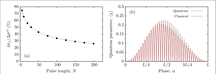
Figure4also shows how the difference between the classical and quantum results increases as the intensity is increased (or asNis decreased). It is therefore interesting to consider the differenceδσˆf =σˆfqm−σˆfclas a

7_{Peak intensity is obtained from}

π ϵ λ λ

= ≃ ×

fraction of the total (constant) classical change in momentum spread,Δσˆcl=σˆi− σˆfcl. This can be found in figure5(a), where we see that forN= 5 the two predictions differ by about 75%. AsNis increased, this ratio is reduced because the average quantum parameter〈 〉χ becomes smaller and radiation reaction is not so heavily suppressed. It would be expected that the two models converge asN→ ∞.

In cases where there is a large discrepancy between the predictions of the two theories, it is especially

important to be confident in the validity of the model. As a semi-classical model, we expect it to remain valid into the weakly quantum regime, such that particles experienceinstantaneousvalues χ2 ≪1_{. Figure5(b) shows the}

evolution of the bunch-average〈 〉χ as the bunch moves through a laser pulse withN= 20 according to the classical and semi-classical models. Initially, there is good agreement between the two models, until the bunch approaches the centre of the pulse, where the intensity becomes higher and the models are significantly different. For completeness, we note that our highest intensity case withN= 5 satisfied〈 〉 <χ2 0.22.

5. Conclusions

[image:12.595.120.552.59.466.2]

The next few years will see the emergence of a number of new high-power laser facilities operating at unprecedentedfield strengths, providing access to fundamentally new physical regimes. This will allow us to experimentally probe previously untested areas of physics, such as the long-standing question of radiation reaction.

In this paper, we have analysed the transverse and longitudinal cooling of a relativistic electron beam as it interacts with an intense laser pulse, according to classical and semi-classical theories of radiation reaction. In the classical theory, we have found these two contributions to be equal, but quantum effects break this symmetry, leading to significantly less cooling in the longitudinal than the transverse directions.

To facilitate evaluation of the longitudinal beam cooling effects, we have introduced an innovative method to efficiently and accurately calculate the distribution function for an electron beam interacting with an intense laser pulse. This has been validated by comparison with an analytical solution to the Vlasov equation in the classical case, and used to compare classical and quantum predictions of radiative cooling. We have found that quantum effects can significantly alter the beam properties and, unlike the classical case, can be influenced by the

shapeof the laser pulse, not just its energy.

As we move into the quantum regime wherefinal-state electron beam properties become sensitive to pulse shape, it is becoming increasingly important to have an efficient method in order to investigate the full

parameter space. The approach developed here to facilitate this study of beam dynamics provides a powerful tool with wide-ranging application within the discipline.

The results presented in this paper are limited to the semi-classical case χ2 ≪1_{. However, it should be}

noted that, for thelongitudinalbeam cooling, this restriction is due to the use of a deterministic equation of motion, and not the method of sampling and reconstructing the distribution. There should be no obstruction to exploring more strongly quantum regimes (such as higher initial beam energies∼5GeV available at ELI) using this approach with a stochastic equation where photon emission probabilities are determined by strongfield QED, as in [29,30]. This will be addressed in future work, along with an investigation of stochastictransverse

beam cooling.

Acknowledgments

This work is supported by the UK EPSRC (Grant EP/J018171/1); the ELI-NP Project; and the European

Commission FP7 projects Laserlab-Europe (Grant 284464) and EuCARD-2 (Grant 312453). Dataset is available online (DOI:10.15129/79f9c58d-7a43-4cc0-a613-ebc028519e5b).

References

[1]www.eli-laser.eu/;www.eli-np.ro/

[2] Lorentz H A 1916The Theory of Electrons and its Applications to the Phenomena of Light and Radiant Heat(New York: Stechert) [3] Abraham M 1932The Classical Theory of Electricity and Magnetism(London: Blackie)

[4] Dirac P A M 1938Proc. R. Soc.A167148 [5] Bhabha H J 1939Proc. R. Soc.A172384 [6] Barut A O 1974Phys. Rev.D103335

[7] Burton D A and Noble A 2014Contemp. Phys.55110–21

[8] Landau L D and Lifshitz E M 1962The Classical Theory of Fields(London: Pergamon) [9] Kravets Y, Noble A and Jaroszynski D A 2013Phys. Rev.E88011201(R)

[10] Spohn H 2000Europhys. Lett.50287

[11] Tamburini M, Pegoraro F, Di Piazza A, Keitel C H and Macchi A 2010New J. Phys.12123005 [12] Sauter F 1931Z. Phys.82742

[image:13.595.119.553.62.212.2]

[13] Schwinger J 1951Phys. Rev.82664 [14] Erber T 1966Mod. Phys. Rev.38626

Figure 5.(a): variation of thefinal relative momentum spread differenceδσˆfas a percentage of the total classical change,Δσˆcl. The

[15] Ritus V I 1985J. Sov. Laser Res.6497_–617

[16] Kirk J G, Bell A R and Arka I 2009Plasma Phys. Control. Fusion51085008

[17] Thomas A G R, Ridgers C P, Bulanov S S, Griffin B J and Mangles S P D 2012Phys. Rev.X2041004 [18] Blackburn T G, Ridgers C P, Kirk J G and Bell A R 2014Phys. Rev. Lett.112015001

[19] Ilderton A and Torgrimsson G 2013Phys. Lett.B725481

[20] Noble A, Burton D A, Gratus J and Jaroszynski D A 2013J. Math. Phys.54043101 [21] Vranic M, Martins J L, Vieira J, Fonseca R A and Silva L O 2014Phys. Rev. Lett.113134801 [22] Burton D A and Noble A 2014Phys. Lett.A3781031

[23] Di Piazza A 2008Lett. Math. Phys.83305

[24] Neitz N and Di Piazza A 2014Phys. Rev.A90022102 [25] Lehmann G and Spatschek K H 2011Phys. Rev.E84046409 [26] Harvey C, Heinzl T and Marklund M 2011Phys. Rev.D84116005

[27] Kravets Y 2014 Radiation reaction in strongfields from an alternative perspectivePhD ThesisUniversity of Strathclyde [28] Neitz N and Di Piazza A 2013Phys. Rev. Lett.111054802