Modification of an asynchronous dexterous hand movement decoder for hardware implementation

Rochester Institute of Technology

RIT Scholar Works

Theses Thesis/Dissertation Collections

6-1-2010

Modification of an asynchronous dexterous hand

movement decoder for hardware implementation

Adam Kevin Bosen

Follow this and additional works at:http://scholarworks.rit.edu/theses

This Thesis is brought to you for free and open access by the Thesis/Dissertation Collections at RIT Scholar Works. It has been accepted for inclusion in Theses by an authorized administrator of RIT Scholar Works. For more information, please [email protected].

Recommended Citation

Modification of an Asynchronous Dexterous Hand

Movement Decoder for Hardware Implementation

by

Adam Kevin Bosen

A Thesis Submitted in Partial Fulfillment of the Requirements for the Degree of Master of Science in Computer Engineering

Supervised by

Associate Professor Daniel B. Phillips Department of Electrical Engineering Kate Gleason College of Engineering

Rochester Institute of Technology Rochester, New York

June 2010

Approved By:

Daniel B. Phillips

Associate Professor, Department of Electrical Engineering Primary Adviser

Juan Carlos Cockburn

Associate Professor, Department of Computer Engineering

Marcin Lukowiak

Thesis Release Permission Form

Rochester Institute of Technology

Kate Gleason College of Engineering

Title: Modification of an Asynchronous Dexterous Hand Movement

De-coder for Hardware Implementation

I, Adam Kevin Bosen, hereby grant permission to the Wallace Memorial Library

repor-duce my thesis in whole or part.

Adam Kevin Bosen

Dedication

I highly doubt I could get away with not dedicating my first major work to my mother, so,

Acknowledgments

Thanks to Marc H. Schieber, who generated the neural data analyzed here and in previous

research on this topic(supported by R01 NS27686).

Thanks to Vikram Aggarwal, Soumyadipta Acharya, and Francesco Tenore for

performing the research that lead to my work and for providing the guidance and advice to

get me going.

Thanks to Daniel Phillips, Juan Cockburn, and Marcin Lukowiak for providing me with

direction and support throughout this research and for happily enduring the many

Abstract

One of the goals of modern prosthetics research is to provide natural, neurologically driven

control of a prosthetic device, preferably in a portable format. Previously, an algorithm for

asynchronously decoding individuated finger and wrist movements from recordings of

neu-ral activity in the primary motor cortex was developed by Aggarwalet al.and implemented

in software. The first objective of this work was to determine what effect simplifying

Aggarwal’s algorithm by using linear Artificial neural networks instead of nonlinear ones

would have on movement detection and classification accuracy. The simplified algorithm

developed in this work was demonstrated to achieve movement detection and

classifica-tion accuracies of 99.7%, 89.9%, and 95.3% for an individuated movement decoding task

across three subjects using neural recordings from 80 neurons. In comparison, the

origi-nal algorithm demonstrated accuracies of 96.2%, 90.5%, and 99.8% for the same task and

subjects using neural recordings from 40 neurons. Additionally, the simplified algorithm

was demonstrated to have a detection and classification accuracy of 80.5% for a combined

movement task, whereas the original algorithm achieved accuracy of 92.5%. Even though

a greater input space size was required for the linear decoder, the computational intensity

was reduced with a mean accuracy loss in the individuated movement task of only 0.53%.

However, the 12% loss of accuracy observed in the combined movement task is considered

unacceptable and suggests that the simplified algorithm is not appropriate for this task.

The second objective of this work was to create a digital hardware implementation of

the simplified linear artificial neural network version of Aggarwal’s algorithm. A scalable,

FPGA. This implementation could be realized with an input dimension of up to 60

neu-rons on this FPGA, although computations were performed on the order of104 _{times faster}

than was necessary for realtime operation, indicating that there is an opportunity to reduce

hardware size in exchange for computational speed. This work is an important exploration

into the eventual goal of incorporating a hardware movement decoder in a prosthetic

de-vice and demonstrates that a hardware implementation is feasible using currently available

Contents

Dedication. . . iii

Acknowledgments . . . iv

Abstract . . . v

1 Introduction. . . 1

1.1 The Nervous System . . . 2

1.2 Recording Nervous Signals . . . 3

1.3 Machine Learning . . . 4

1.4 Asynchronous Dexterous Decoder . . . 8

1.5 Thesis Objective . . . 12

2 Algorithm Modifications . . . 14

2.1 Replacement of Nonlinear Artificial Neural Networks . . . 15

2.2 Gating Logic Modification . . . 17

2.3 Elimination of Floating Point Multiplication . . . 22

3 Hardware Implementation . . . 26

3.1 Architecture Selection and Requirements . . . 26

3.2 Choice of a Development Platform . . . 28

3.3 Hardware Implementation Overview . . . 30

3.4 Input Window . . . 31

3.5 Classifiers . . . 32

3.6 Output Logic . . . 33

3.7 IO Interface . . . 34

3.8 Hardware Analysis . . . 36

4 Test Methodology . . . 39

4.2 Classifier testing . . . 41

4.3 Comparing Hardware and Software Implementations . . . 42

5 Results. . . 43

6 Discussion . . . 49

6.1 Algorithm Modification Analysis . . . 49

6.2 Hardware Implementation Analysis . . . 51

7 Conclusions . . . 55

List of Figures

1.1 Example of a simple artificial neural network with three inputs, a single hidden layer, and one output. Each node, represented by circles, computes the weighted sum of each input, represented by arrows. . . 6 1.2 A diagram of the original asynchronous dexterous decoder[1]. The use

of two classifiers allows for the detection and classification of movement from recorded nerual signals,X(tk), without any reliance on external cu-ing. The gating classifier output, G(tk), is a boolean value that corre-sponds to whether or not movement is occurring, with the heuristic check,

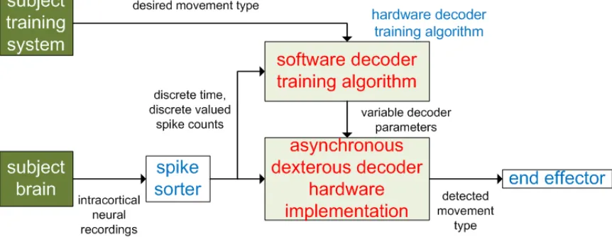
Gtrack(tk), eliminating spurious classifications. The movement classifier output,S(tk), represents which type of movement, out of a predefined set, is occurring. Together, they allow for the asynchronous detection of a spec-ified set of finger and wrist movements from the recorded firing rates of neurons in the primary motor cortex[1]. . . 11 1.3 Block diagram of a complete neurally controlled hand prosthesis. White

text indicates preexisting structures, red text indicates the proposed work, and blue text indicates additional components necessary for a complete portable neurally controlled hand prosthesis. . . 13

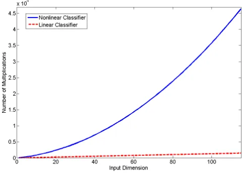
2.1 Number of multiplications required per classification with respect to input space dimension, assuming the nonlinear classifier uses an average hidden layer size 1.5 times larger than the input space and a 12 movement output space. . . 16 2.2 Response of linear gating classifier to a set of four movements occurring

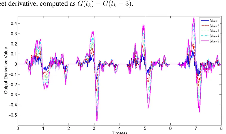
2.3 The discrete derivative of the gating classifier response to a set of four movements using the entire input space, computed asG(tk)−G(tk−∆), where∆ranges from 1 to 5. Movements occurred at times 1, 3, 5, and 7 seconds, to which the negative signal peaks correspond (the peak observed near time 2 seconds is a false positive). Note that as∆increases both the peak magnitude and delay between movement time and peak time increase. 19 2.4 Response of linear gating classifier to a set of four movements occurring

once every two seconds using the entire input space with gating classifier derivative. The blue solid line represents the function that the gating classi-fier was trained to, the red dashed line represents the actual response of the gating classifier, and the green line represents the discrete time derivative

of the gating classifier response. . . 20

2.5 Response of linear movement classifier to a sequence of trials occurring once every two seconds using the entire input space. The movements were presented every odd second in the following order: extension of each digit, in order from thumb to little finger (e1-e5), extension of the wrist(ew), flexion of each digit in the same order(f1-f5), and flexion of the wrist(fw). The diagonal row of spikes in the center of the diagram shows that the largest response during each trial is the expected movement type. . . 21

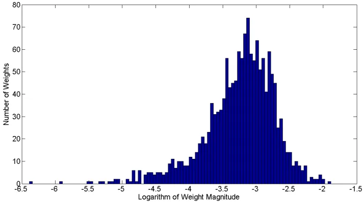
2.6 This graph shows the base-10 logarithm of a sample distribution of classi-fier weights after training to a full input space (1495 weights total). . . 22

3.1 Block diagram of input window . . . 31

3.2 Block diagram of linear classifiers . . . 32

3.3 Block diagram of gating logic . . . 33

3.4 Block diagram of movement logic . . . 34

3.5 Block diagram of output logic . . . 35

3.6 Block diagram of asynchronous dexterous decoder hardware implementa-tion with IO interface . . . 36

3.7 Critical path delay with respect to input space dimension. Note that since the graph scale is on the order of nanoseconds the 20ms maximum is not an issue. . . 37

5.1 Movement detection accuracy rate of the gating classifier with respect to the level threshold and derivative threshold parametersγandδin the region 0.2≤γ ≤0.5,−0.1≤δ≤0. . . 44 5.2 Movement detection accuracy rate of the gating classifier with respect to

the level threshold and derivative threshold parametersγandδin the region 0.25≤γ ≤0.35,−0.06≤δ≤ −0.01. . . 44 5.3 False Positive rate of gating classifier with respect to the gating classifier

refractory period parameterρ. . . 44 5.4 Linear classifier decoding accuracy with respect to input space size. Note

List of Tables

5.1 Summary of gating classifier accuracy using the full input space of each subject. . . 45 5.2 Summary of movement classifier accuracy using the full input space of

each subject. . . 45 5.3 Table of output differences between hardware and software implementation

over 100 trials with an input dimension of 10. . . 46 5.4 Table of output differences between hardware and software implementation

over 100 trials with an input dimension of 20. . . 47 5.5 Table of output differences between hardware and software implementation

over 100 trials with an input dimension of 30. . . 47 5.6 Table of output differences between hardware and software implementation

over 100 trials with an input dimension of 40. . . 48 5.7 Table of output differences between hardware and software implementation

over 100 trials with an input dimension of 50. . . 48

Chapter 1

Introduction

One of the primary problems in prosthetics development is the need for a means of control

that functions similarly to the biological system the prosthetic is intended to replace. Recent

research has focused on brain-machine interfaces (BMI), which is the recording and

decod-ing of electrophysiological measures of neural activity to control an electronic device[1].

The nervous system has several unique properties that must be accounted for when

design-ing a BMI. One of these properties is the duplication of signals in multiple locations in

the body, which has allowed researchers to explore multiple methods of recording nervous

information[2, 3]. This also means that it is often very difficult to isolate a single signal

re-sponsible for any individual action, so machine learning techniques are typically employed

to convert neural recordings to useful information. One method of performing this, the

asynchronous dexterous decoder developed by Aggerwalet al.[1], is the foundation of the

research presented in this paper. This algorithm has been previously demonstrated to be

capable of asynchronously detecting and identifying hand movements in rhesus monkeys

with as high as a 99.8% accuracy[1], indicating that it is potentially viable for use in a hand

prosthesis. The goal of this research is to develop a simplified version of the asynchronous

dexterous decoder that requires fewer computational resources per classification decision,

quantify the accuracy of the simplified decoder, and design and implement a hardware

1.1

The Nervous System

In order to meet the objective of this research it is necessary to understand the structure of

the nervous system and the nature of the signals it generates. The nervous system is one

of the primary organ systems responsible for control and communication between all other

systems in the body. Its functions include sensory integration and motor control, along

with cognition. The functional units of the nervous system are nerves, which are bundles

of specialized excitable cells called neurons that can accept and propagate signals through

the body[4].

The primary means of signal propagation in an individual neuron is the action potential,

a rapid depolarization and repolarization of the electrical potential between the interior and

exterior of the neuron[5]. A depolarization in one part of the cell will cause depolarization

of adjacent portions of the cell, effectively allowing for the action potential to travel down

the cell. Action potentials typically have a amplitude of +100mV and can occur at a

max-imum rate of 200Hz[5]. Since the amplitude of an action potential is fixed, information is

encoded in the rate at which the action potentials occur. The rate at which action

poten-tials occur is limited by the presence of a refractory period following each action potential,

during which another action potential cannot occur[4].

Individual neurons are bundled in groups called nerves which are responsible for

trans-mitting information through the body. Any nerve not located in the brain or spinal cord

are designated as part of the peripheral nervous system (PNS), while the brain and spinal

cord are collectively known as the central nervous system (CNS). The PNS is primarily

responsible for propagation of sensory and motor information, while the CNS performs

most decision making and control signal generation tasks. The brain is divided into several

distinct components, each of which is primarily responsible for different aspects of mental

function, including sensory integration, cognition, and control of autonomic processes. The

outer layer of neurons in the brain, the cerebral cortex, plays a significant role in perception,

The cerebral cortex can be divided into regions called Brodmann areas that are

pri-marily responsible for specific functions[4]. Communication in these area is performed by

ensembles of neurons firing together, so recording from any portion of one of these areas

should give a good overall representation of the area’s current activity. The function of an

individual neuron in one of these areas may change over time, but the overall function of

the area remains fairly constant[4].

One Brodmann area of particular interest for this research is the primary motor cortex,

which is responsible for voluntary movement. Control of every portion of the body is

mapped topographically to the primary motor cortex, so recording the activity of a portion

of the primary motor cortex can provide relevant information about what the corresponding

portion of the body is doing[4]. Research has demonstrated that sufficient information to

decode the movement of individual fingers is distributed throughout the hand control region

of the primary motor cortex, so neural recordings taken from any portion of this region can

provide a good representation of overall hand activity[3].

1.2

Recording Nervous Signals

In order to make use of the information available in the nervous system a means of

record-ing and interpretrecord-ing its signals is necessary. Several methods of performrecord-ing this task are

currently being researched, one of which is electrode implantation. As the name implies,

this method involves directly implanting electrodes into some section of the brain for the

purpose of recording neural signals. Typically, recording is done using a cluster of

elec-trodes arranged in an array suitable for implantation in one specific portion of the brain[6].

Research has shown that recording as few as 20 neural signals located anywhere within

the hand area of the primary motor cortex is sufficient to provide a reliable estimate of

hand activity[3], although the most common type of electrode array, the Utah Intracortical

Electrode Array, is capable of recording significantly more[6]. Individual electrodes in the

but several filtering and sorting algorithms known collectively as spike sorters have been

developed to address this issue[7, 8]. Additionally, long term studies have been performed

on electrode arrays that demonstrate they can maintain signal quality for a period of at least

1.5 years, which shows potential for use in long term applications[9]. The specific

record-ing areas, significant quantity of data, and long term durability make this approach viable

for prosthetic control.

However, electrode implantation does have a few significant limitations. The biggest

barrier to this approach is the need to directly implant the electrodes into the brain, which

requires significant surgery to remove the skin, bone, and meninges directly over the desired

recording site [6]. This surgical procedure has been performed on cats[6] and monkeys[1],

but obvious ethical considerations prevent much experimentation on humans. Additionally,

the function of individual neurons is known to potentially shift over time[9], so systems

designed to use information recorded from an electrode array will need to be capable of

accounting for this shift.

1.3

Machine Learning

Once nervous signals are obtained from a subject, they can be processed using machine

learning. Machine learning is the study of algorithms that can learn rules based on example

data[10]. It is often used to create rules that relate data sets in situations where the

relation-ship between those sets is not well understood. In the context of brain-machine interfacing,

machine learning can be applied to create rules that relate nervous activity to observed body

function. The ability to generate relationships between data sets is of particular value in

this application due to the fact that the exact function of any individual nervous signal is

often difficult to determine. In general, there is no guarantee that a relationship between a

set of nervous signals and body function exists, but previous research has demonstrated that

activity in the hand control region of the primary motor cortex can be mapped to a set of

creating a relationship between two data sets[11]. One approach, artificial neural networks,

can be used to create mappings of arbitrary complexity from one data set to another and

are capable of defining complex, nonlinear relationships.

An Artificial Neural Network (ANN) is a directed graph where each node computes a

weighted sum of its inputs. An ANN consists of external inputs from one data set, weighted

connections between nodes, and external outputs that represent the network’s mapping into

a different set. The complexity and linearity of the mapping performed by the ANN is

controlled by the number of nodes and the way they are connected, while the exact shape

is determined by the weight values. Mapping an input set to an output set is performed

via training, which uses presented data to adjust network weights. Although ANNs can be

constructed arbitrarily, in this work only layered feedforward networks will be considered

in order to avoid introducing the increased complexity of time variant systems. A

feedfor-ward network consists of two or more discrete layers of neurons in which every node of

one layer functions as an input to every node in the next layer. The first layer is the input

layer, where system inputs are directly applied, and the last layer is the output layer, where

the output values are read from. Additional layers between the input and output layers are

referred to as hidden layers, because they are not directly controlled or visible outside the

ANN. In hidden layers a nonlinear function, typically a sigmoid or a hyperbolic tangent is

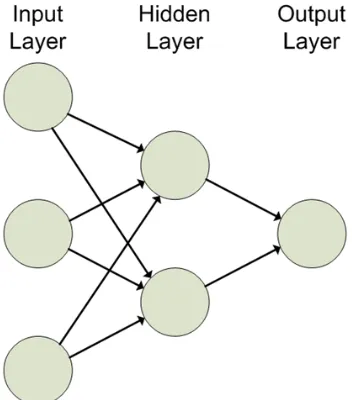
applied to each sum to allow for the ANN to produce nonlinear mappings[10]. Figure 1.1

shows a diagram of a simple ANN consisting of three inputs, a single hidden layer with

two nodes, and a single output.

Each connection from one layer to the next can be viewed as a transform from one space

to another. If no hidden layers are present in the ANN then the relationship between the

inputs and an individual output can be expressed simply as a weighted sum and is therefore

linear. Geometrically, this describes a hyperplane drawn through the input space. The

dis-tance from a point in the input space to this plane determines the value of the corresponding

output of the ANN. Alternatively, if hidden layers are used then the transformation from

Figure 1.1: Example of a simple artificial neural network with three inputs, a single hidden layer, and one output. Each node, represented by circles, computes the weighted sum of each input, represented by arrows.

that a nonlinear function is applied to each sum. If this nonlinear function was not present

the ANN would be several cascaded linear transforms, which could be simplified to a

sin-gle linear transform and render it unable to perform higher order functions. Nonlinearity is

advantageous because it allows for mappings that are not possible with a linear transform,

although additional computation is required to perform this mapping. Each hidden layer

increases the order of the mapping function, which can allow for mappings that would not

be attainable with a lower order function[10].

For the sake of simplicity it is preferable to use the least computationally intensive ANN

that meets performance requirements. The number of hidden layers and hidden nodes in

an ANN determine the order of complexity of the functions it is capable of learning as

well as the number of calculations required to compute a result[10]. Therefore, there is a

tradeoff between accuracy and computational cost that is governed by hidden layer size and

quantity. An ANN with no hidden layers is only capable of computing linear functions,

but only requires a number of computations of order n, wheren is the input dimension.

each hidden layer, but requires a number of computations of order nm_{, where m is the}

number of hidden layers. Additionally, each hidden layer requires the computation of a

nonlinear function for each sum. This tradeoff indicates that it is desirable to find the

smallest ANN that is capable of estimating the desired function to a specified accuracy. If

problem complexity is unknown, as is the case for many machine learning applications,

then using an ANN with more hidden layers or nodes than necessary will not adversely

affect performance, but will be more computationally intensive than necessary.

One of the objectives for any machine learning task is the minimization of output error.

Typically, this requires that the system be trained using sample data. One of the common

methods of training an ANN is gradient descent. Gradient descent is a supervised learning

algorithm that minimizes error by descending the gradient of the mean square error between

the actual and desired outputs. In an ANN with no hidden layers this is done by giving the

system an input value, comparing the system output to the desired output, and modifying

the weights in the weight vector by subtracting from it the partial derivative of the error

with respect to that weight multiplied by a learning factor. In this method, weights that

have a greater contribution to the incorrect value are modified more heavily. As the system

is trained the learning factor is gradually decreased in order to converge on a single set of

weights for the system. Equation 1.1 expresses this rule mathematically, where∆wt j is the

amount added to weightwj after training examplet, ηis the learning factor that controls

the magnitude of weight adjustments, rt _{is the desired output at training example t, y}t _is

the actual output at training examplet, andxt_j is the input corresponding to weightwj[10].

∆w_jt =η(rt−yt)xt_j (1.1)

For an ANN with hidden layers gradient descent is performed via backpropagation, which

essentially performs the same weight modifications one layer at a time. The output layer is

modified in a manner identical to gradient descent, and previous layers are iteratively

mod-ified after determining the amount of error each neuron in the previous layer contributed.

Note that in order for this to be possible the output of every neuron needs to be

layer[10].

Another potential goal for a machine learning task that has a large number of inputs is

to reduce the number of inputs to a smaller subset that still meet performance requirements.

This is especially useful when it is suspected that some inputs provide information that is

redundant or independent of the desired output function. Reduction of system complexity

can be accomplished by incorporating a method of structural adaptation into the learning

algorithm. This can be either constructive, where inputs are added to a very simple

net-work as needed, or destructive, where inputs are removed from a complex netnet-work as they

are determined to be unnecessary. One simple method of destructive reduction is weight

decay. Weight decay replaces the error function used for gradient descent with an error

function that penalizes output error andweight size. This gives each weight in the system

a tendency to decay to zero. If a particular input associated with a weight is not necessary

to provide accurate classification then its contribution to the system is removed without

af-fecting overall accuracy. Input weights that are critical to correct classification are updated

whenever an error occurs, so their weights are not removed. At the end of training, any

inputs with weights of zero can be removed without affecting classifier accuracy[10].

1.4

Asynchronous Dexterous Decoder

The asynchronous dexterous decoder developed by Aggarwalet al.is a system for decoding

a specific set of hand movements from neural signals recorded from the primary motor

cortex. This decoder uses committees of artificial neural networks to detect and classify

finger and wrist extension and flexion from intracortical neural signal recordings. It was

demonstrated to be accurate over 90% of the time in three different subjects, indicating that

it is a potentially viable for use in a neurally controlled multifingered hand prosthesis[1].

The data used for this work were intracortical neural signals recorded from three male

rhesus monkeys, identified as monkeys C, G, and K. Each monkey was trained to perform

performing these movements, a recording was obtained from a single neuron in the

pri-mary motor cortex. Each subject had different numbers of recording sites: 312 neurons

were recorded from in monkey C, 125 neurons were recorded from in monkey G, and 115

neurons were recorded from in monkey K. Data was collected from each neuron

individ-ually in a series of repeated trials for each movement type. For monkeys C and G up to

seven trials were recorded for each neuron for each movement type, while for monkey K

up to 15 trials were recorded per neuron per movement type. These recordings were then

processed by a spike detector that quantified the time at which action potentials occurred

with respect to time at which a movement was performed[1].

The feature that makes this decoder unique is its asynchronous nature. Most prior

research focused on cued decoding, which relies on an external signal to indicate when

decoding should be performed. Obviously, this dependence is undesirable when attempting

to develop a useful prosthetic device. The asynchronous dexterous decoder overcomes this

limitation by using two classifiers: one classifier determines whether or not a movement

is occurring (gating classifier), and the other determines what type of movement out of a

specified set is being performed (movement classifier). Input to both classifiers is provided

as a count of the number of action potentials that occur during a 100ms window that shifts

forward every 20ms. This sliding window produces a set of discrete time, discrete valued

signals that describe the activity of each neuron in the system[1].

As shown in figure 1.2, the gating classifier was designed as a odd numbered committee

of artificial neural networks trained to produce an output between 0 and 1 corresponding to

the probability that movement was occurring. Each ANN possessed a single tan-sigmoidal

hidden layer containing anywhere from 0.5 to 2.5 times the number of input neurons, a

single output neuron, and a log-sigmoidal output function. The output of each ANN was

thresholded at a value of γ to produce a boolean value of 0 or 1. A majority voting rule

was used to determine the committee output. If the committee output was 1 more thanβ

times in the pastτ decisions then the gating classifier fired, indicating positive movement.

to guard against false positives[1]. This rule is expressed mathematically in equation 1.2,

whereG(tk)is the gating ANN committee output andGout(tk)is the movement detection

decision, with a 1 indicating movement and a 0 indicating no movement.

Gout(t) =

    

1 ifPtk

t=tk−τG(tk)> β

0 otherwise

(1.2)

Like the gating classifier, the movement classifier consists of an odd numbered

com-mittee of ANNs, but each ANN had a number of output neurons equal to the number of

movement types decoded, with each neuron corresponding to a specific movement type.

A set of twelve distinct movement types were performed in all subjects: flexion and

ex-tension of each individual finger and the wrist. In one subject, monkey K, additional data

was recorded for an extra set of six movement types: combined flexion and extension of

the thumb and forefinger, the forefinger and middle finger, and ring finger and little finger.

Every movement type was treated as a binary decision, with no consideration given to

par-tial movements. Each ANN was trained to output values between 0 and 1 corresponding

to the probability that a given movement type was occurring. The movement type with the

highest probability was chosen as the output of each network, and a majority voting rule

was used to determine the movement classifier output[1]. Equation 1.3 expresses this rule

mathematically, wheres(t)is the movement decision out of the set ofimovements at time

tandPi(t)is the output of movement ANNiat timet.

s(t) = arg max

i Pi(t) (1.3)

The final classification decision was produced by multiplying the output of the gating

classifier with the output of the movement classifier. Ideally, this produces an output of

zero when no movement is detected and an integer corresponding to a specific movement

type when that movement type is detected. A diagram of the decoder is shown in figure 1.2

All portions of the decoder were implemented and trained in software using Matlab[1].

Figure 1.2: A diagram of the original asynchronous dexterous decoder[1]. The use of two classifiers allows for the detection and classification of movement from recorded nerual signals,X(tk), without any reliance on external cuing. The gating classifier output,G(tk), is a boolean value that corresponds to whether or not movement is occurring, with the heuristic check, Gtrack(tk), eliminating spurious classifications. The movement classifier output, S(tk), represents which type of movement, out of a predefined set, is occurring. Together, they allow for the asynchronous detection of a specified set of finger and wrist movements from the recorded firing rates of neurons in the primary motor cortex[1].

for all three subjects when as few as 40 neurons were used as input. Additionally, the

decoder was shown to be as high as 99.8% accurate for monkey K in the individual finger

movement task and 92.5% accurate for monkey K when combined movements were added

to the output space. These results demonstrate that this algorithm is robust to decode hand

movements regardless of the specific neural population recorded from, which indicates that

it has potential application to the development of a neurally controlled hand prosthesis[1].

Additionally, research by Acharyaet al.[3] demonstrates that movement can be accurately

neurons contain some redundant information. Since it is known that a good nonlinear

approximation exists when 20 neurons are used adding information from other neurons can

be viewed as a transformation to a higher dimensional space, which may allow classes to be

separated linearly[10]. However, since the exact transformation that occurs when neurons

are added is unknown, linearly separability cannot be guaranteed, but the possibility that

linear separability exists for this problem was investigated because it would allow for the

order of complexity of the ANNs in the asynchronous dexterous decoder to be reduced.

1.5

Thesis Objective

The purpose of this research is to determine if an asynchronous dexterous decoder that

uses only linear ANNs can achieve accuracy comparable to that of the original decoder

presented in [1] and, if so, implement the linear ANN decoder in digital hardware.

Ide-ally, the linear ANN decoder will be as accurate as the nonlinear ANN decoder, although

accuracy degredation is acceptable if the best case decoder accuracy does not fall below

90%, which is comparable to the lowest best case performance demonstrated by the

origi-nal nonlinear ANN decoder. It is proposed that meeting this accuracy objective will require

a larger input space than necessary for comparable accuracy in the nonlinear ANN

de-coder. This requirement is considered acceptable, because even if the linear ANN decoder

requires a larger input space, the order of complexity will still be lower than that for the

nonlinear ANN decoder. If this accuracy objective can be met, the linear ANN decoder

would be adapted for a digital implementation capable of making classification decisions

in real time, which was defined in the original algorithm as one decision every 20ms.

The implementation of a digital realization of the asynchronous dexterous decoder is

an important step toward a practical prosthesis, but it is beyond the scope of this work to

develop a completely independent prosthetic control system. All ANN training will be

per-formed in software using MATLAB (Mathworks Inc., Natick, MA) using custom scripts

feasibility of implementing a hardware based machine learning system will be performed

as a basis for potential future work. Additionally, the data used to train and test the system

will be the discrete time, discrete valued integer counts of the number of action

poten-tials(spikes) that occurred in the past 100ms, moving forward every 20ms, as described in

section 1.4. In a complete neurally controlled prosthesis this information would need to be

extracted from neural recordings by spike sorting and counting hardware, then provided to

the asynchronous dexterous decoder. Several algorithms for the detection of action

poten-tials that would be suitable for incorporation into a neurally controlled prosthesis have been

developed previously[12, 13], indicating that this requirement is not a major limitation on

future work. The other necessary component of a neurally controlled prosthesis, the end

ef-fector, will not be integrated with the asynchronous dexterous decoder in this work. Figure

1.5 shows a block diagram of a complete neurally controlled hand prosthesis and the way

in which the research performed in this thesis is meant to be incorporated into a complete

prosthetic system.

Chapter 2

Algorithm Modifications

The first objective of this research is to determine if the asynchronous dexterous decoder

algorithm can be modified to use linear artificial neural networks while still meeting the

accuracy requirements defined previously. This chapter describes the theoretical

modifica-tions made to the asynchronous dexterous decoder algorithm and their impact on the

com-putational complexity of the system. For a digital hardware implementation of an ANN

the number of floating point multiplications necessary to compute the output is the most

intensive aspect of the algorithm[14], so computational complexity of the decoder will be

primarily measured in terms of number of floating point multiplications. The four

modifi-cations made to the decoder algorithm were the replacement of the nonlinear ANNs with

linear ANNs, the removal of the committee voting structure, a new gating decision

algo-rithm, and an integer approximation of all floating point math. These modifications

pur-posefully do not include any changes to the sliding input window or decision rate, so that

any larger system can use the original decoder algorithm developed by Agarwalet al.or the

new, modified algorithm interchangeably, and to simplify direct comparison between the

two algorithms. All modifications were designed with the intention of providing the same

movement classification accuracy as the original algorithm at a reduced computational cost.

Since the functionality of the original algorithm is only approximated some error is

intro-duced, although attempts were made to minimize its impact on movement classification

accuracy. All training and testing computations described in this chapter were performed

2.1

Replacement of Nonlinear Artificial Neural Networks

The first modification performed on the decoder algorithm was the replacement of the

non-linear, single hidden layer ANNs with linear ANNs. The purpose of this modification was

to determine if the same classification accuracy can be achieved at a lower computational

cost. The switch from a nonlinear ANN to a linear ANN can be viewed as simply removing

the hidden layers from the ANN. Removing hidden layers imposes a significant constraint

because it restricts the ANN to only linear transformations, but if linear separability can be

demonstrated then this constraint will not adversely affect performance.

Switching from nonlinear ANNs to linear ANNs reduces the usefulness of the

commit-tee voting structure used in the original algorithm. An ANN with hidden layers inherently

implements a nonlinear function, so more than one function that can approximate the

de-sired output may exist. Additionally, the number of nodes in a hidden layer may be varied,

so multiple ANNs, each with a different number of hidden layer nodes, can be combined in

a committee structure to yield accuracy greater than each ANN individually[1]. In

compar-ison, an ANN without hidden layers is only capable of implementing linear functions. This

limitation means there will only be one error minimum towards which all stable learning

algorithms will converge. Therefore, every member in a committee of linear ANNs would

appear to be almost identical, which eliminates the utility of the committee. Based on this

fact, it was decided a single linear ANN was sufficient to replace each committee.

In terms of computational complexity, the single most prevalent and expensive

oper-ation in the implementoper-ation of an ANN is floating point multiplicoper-ation. A multiplicoper-ation

is needed for each connection from one layer to the next, from which the total number

can be determined as the product of the number of neurons in each layer. For example,

a typical implementation of the original asynchronous dexterous decoder uses about 40

input neurons, 3 committees for each classifier, and 12 movement types. Assuming the

mean number of hidden layer neurons of 1.5 times the number of input neurons gives an

estimated need for ((40 input neurons)(60 hidden neurons)+(60 hidden neurons)(12 output

classifier and ((40 input neurons)(60 hidden neurons)+(60 hidden neurons)(1 output

neu-ron))(3 ANNs in each committee) = 7,380 floating point multipliers for the gating classifier.

This gives a combined total of 16,740 floating point multiplications needed for the

origi-nal algorithm for each classification decision. In comparison, the number of multipliers

needed for a linear, committee-less algorithm is (40 input weights)(1 linear classifier) =

40 multipliers for the gating classifier and (40 input weights)(12 movement types)(1 linear

classifier) = 480 multipliers. This gives a total of 520 multipliers, which is still about 35

times fewer than the neural network. Furthermore, the lack of a hidden layer means that

the number of multiplications required to calculate a classification scales linearly with

in-put dimension, unlike the nonlinear ANN approach, where the number of multiplications

required increases as the square of the input dimension. Figure 2.1 compares the relative

complexity (number of multiplications required per classification) of each classification

al-gorithm with respect to the size of the input space. Note that, despite the change in the

way computations are performed, the input and output, a count of the number of spikes

for each neuron in the past 100ms and an integer corresponding to a classification

deci-sion, are untouched, so from an external perspective the linear and nonlinear classifiers are

interchangable.

2.2

Gating Logic Modification

Ideally, the above changes should not have significantly impacted classifier performance.

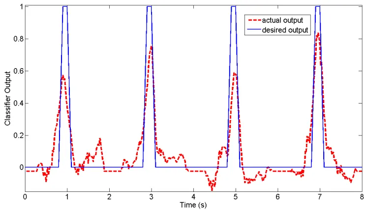
However, it was observed in early testing that this was not the case. Figure 2.2 shows

the output of the new, linear gating classifier in response to a set of four movement trials

occurring once every two seconds. The variation in the shape of this output was observed

to be typical for the gating classifier. As shown, the gating classifier output does not closely

follow the desired output, in one case rising only as high as 0.58 instead of the desired value

of 1, but does demonstrate a rising and falling pattern that roughly follows the rise and fall

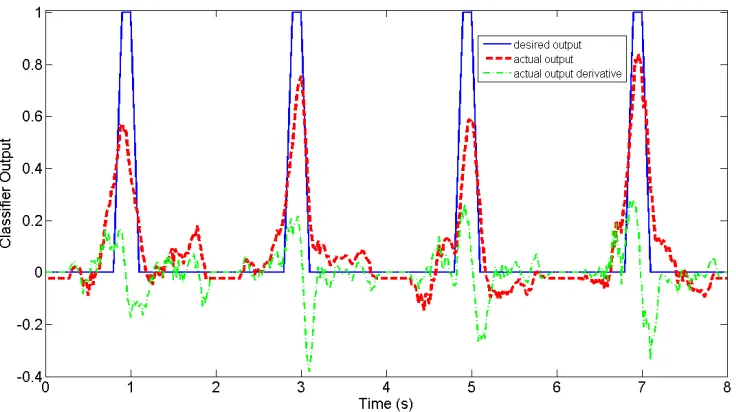
of the desired output. The potential reason for these variations is discussed later.

Figure 2.2: Response of linear gating classifier to a set of four movements occurring once every two seconds using the entire input space. The blue solid line (desired output) rep-resents the ideal signal that the gating classifier was trained to, and the red dashed line (actual output) represents the actual response of the gating classifier. Note that the peak level, duration, and location with respect to the desired output is not consistent from trial to trial.

The error demonstrated in figure 2.2 by the gating classifier is undesirable. The peak

level, time, and duration are not consistant from trial to trial, and the classifier output

wanders (even taking negative values) when no activity is present. If the primary objective

be discarded in favor of a different solution. However, the goal of this classifier is to

provide enough information to allow a decision making scheme to accurately determine

when a movement occurs. Based on the clear presence of output activity at the desired

times an alternative decision making rule was designed.

As described previously, the original algorithm used a movement detection scheme that

counted the number of times the gating classifier output was above a static threshold in a

set window and fired if the output was above the threshold above a certain number of times.

This approach was sufficient for the nonlinear classification scheme because the nonlinear

gating classifier closely and predictably followed the desired output, but since the linear

gating classifier did not consistently reach a specific peak value for a predictable duration

this decision scheme was not as effective. A four dimensional search of the parametersγ,

τ,β, andρwas performed (values ranged between 0.15 to 1 in 0.05 increments forγ, 3 to

10 in integer increments forτ andβ, and 2 to 10 in integer increments forρ) to find

param-eter values that met the specified accuracy requirements, but a set of values that achieved

at least 90% movement detection accuracy was not found. As a result, an alternative

de-cision method was developed. Analysis of the problem showed that although the gating

classifier output did not peak consistently, it did drop off rapidly following a movement.

This lead to the decision to use the derivative of the gating classifier output as well as the

output itself. Figure 2.3 shows the derivative of the actual response signal from figure 2.2,

computed as G(tk)−G(tk−∆), where ∆ranged from 1 to 5. The important aspect of these signals is the negative peaks, which correspond to a decrease in the gating classifier

output, indicating that a movement occurred. As∆increases the magnitude of the negative

peaks increases, along with the delay between the actual movement time and peak time.

This relationship creates a tradeoff between movement identifiability and temporal

accu-racy. To compromise, a value of∆ = 3was selected, creating a delay of three time samples

(60ms) and negative peaks that are sufficiently large to detect movement (Determination of

exact threshold levels is discussed later, in chapter 4). Further analysis of figure 2.3 shows

peaks, such as the one slightly before the two second mark, are present in the signal even

when no movement is occurring. Because of this, the decision was made to use both the

gating classifier output and its derivative to detect movement. Figure 2.4 shows the same

movement response as in figure 2.2 with added information of the gating classifier output

discreet derivative, computed asG(tk)−G(tk−3).

Figure 2.3: The discrete derivative of the gating classifier response to a set of four move-ments using the entire input space, computed asG(tk)−G(tk−∆), where∆ranges from 1 to 5. Movements occurred at times 1, 3, 5, and 7 seconds, to which the negative signal peaks correspond (the peak observed near time 2 seconds is a false positive). Note that as∆increases both the peak magnitude and delay between movement time and peak time increase.

Based on this, the new movement detection decision scheme was designed to check if

the output was above some static threshold γ and instead of counting the number of time

windows during which the output was above this threshold also checked the derivative of

the gating classifier output. If the difference between the current output and the output three

time windows ago was less than the negative constantδ and the current output was above

the thresholdγ the gating classifier fired. Equation 2.1 expresses this rule mathematically,

where γ and δ are the parameters described above, G(t) is the gating classifier output

Figure 2.4: Response of linear gating classifier to a set of four movements occurring once every two seconds using the entire input space with gating classifier derivative. The blue solid line represents the function that the gating classifier was trained to, the red dashed line represents the actual response of the gating classifier, and the green line represents the discrete time derivative of the gating classifier response.

indicating no movement.

Gout(t) =

    

1 ifG(t)> γandG(t)−G(t−3)< δ

0 otherwise

(2.1)

One additional issue highlighted by figure 2.4 is that the criteria for movement detection

defined in equation 2.1 can be true for more than one classification decision during each

movement trial. Every time the gating classifier fires it is considered a separate detection

of movement, which could lead to the misclassification of a single movement as multiple

movements. To reduce this occurrence a refractory period was added. Once the gating

classifier output a positive movement decision, further positive decisions were ignored until

at leastρtime steps had occurred.

The output of the movement classifier was also observed to determine if it still

per-formed similarly to the original algorithm. Figure 2.5 shows the response of the movement

classifier to a sequence of 12 movements occurring once every two seconds in the following

Figure 2.5: Response of linear movement classifier to a sequence of trials occurring once every two seconds using the entire input space. The movements were presented every odd second in the following order: extension of each digit, in order from thumb to little finger (e1-e5), extension of the wrist(ew), flexion of each digit in the same order(f1-f5), and flexion of the wrist(fw). The diagonal row of spikes in the center of the diagram shows that the largest response during each trial is the expected movement type.

wrist(ew), flexion of each digit in the same order(f1-f5), and flexion of the wrist(fw). The

desired output for this trial is a series of output spikes that have a value of 1 when the

cor-responding movement is being performed and 0 all other times. As shown in the diagram,

the response does not closely follow this desired output, instead peaking at a maximum of

0.32, but as in the gating classifier, enough information is still present to make a correct

decision. As mentioned previously, the movement classifier output is only used when the

gating classifier determines that a movement has occurred. As shown in this graph, at the

time a movement occurs there is a clear spike from the desired movement type, while all

other movement types show little activity. This demonstrates that choosing the movement

type with the largest corresponding movement classifier output when the gating classifier

fires will provide a correct movement classification. This rule is expressed mathematically

in equation 2.2, wherePi(t)is the output corresponding to each movement typeiands(t)

is the chosen movement type.

s(t) = arg max

2.3

Elimination of Floating Point Multiplication

Even with a reduced number of floating point multiplications this operation still represents

the most computationally intensive portion of the algorithm. Fortunately, analysis of the

decoder algorithm shows that floating point math can be completely replaced by integer

math without introducing error sufficient to adversely affect classification decisions. Initial

analysis of weights in the gating and movement classifier after training with a full input

space showed that weights differed by several orders of magnitude, although the

major-ity were less than 10−3. Figure 2.6 shows the magnitude logarithm of an example set of

post-training weights. Examination of this figure suggests that weight magnitudes are

ap-proximately log-normally distributed. The fact that the order of magnitude of the weights

roughly falls in this distibution indicates that an approximation of these weights needs to

primarily focus on preserving the accuracy of the weights closer in order to the mean. In

this set of weights, the magnitude mean was9.98∗10−4_{and the magnitude standard}

devia-tion was1.2∗10−3, with minimum and maximum magnitudes of4.11∗10−7and1.3∗10−2. This range of about five orders of magnitude was typical, although exact values varied each

time the system was trained.

With this distribution in mind a simplification that eliminated floating point

multiplica-tions was derived. Generally, a linear classifier can be described by equation 2.3, where n

is the number of inputs,wis the constant weight multiplied by each inputx,bis a constant

offset, andyis the classifier output.

y= n

X

i=0

wixi+b (2.3)

For this specific problem it is known that all inputsxare nonnegative integers with a

max-imum value of about 20, due to the limiting effect of refractory periods. The weights are

floating point numbers and are on the order of10−2_to10−7_{, which makes direct rounding}

them a poor idea. However, scaling by a large constant α (henceforth referred to as the

rounding coefficient) reduces the error introduced by rounding.

αy= n

X

i=0

αwixi+αb (2.4)

Note that in this stateαwi is still a floating point number. To simplify, a new valuewˆi that

is the nearest integer toαwiis substituted into the equation.

ˆ

wi =round(αwi) (2.5)

αyˆ= n

X

i=0

ˆ

wixi+αb (2.6)

This substitution effectively eliminates the need for floating point multiplication. To prove

that this introduces negligible error rounding can be modeled as a uniform error between

-0.5 and 0.5, assuming that the value of the rounding coefficient is large enough that every

weight has a magnitude of at least 1, and the value ofyˆcan be compared toy.

ˆ

wi =αwi+U(−0.5,0.5) (2.7)

Substituting this distribution into equation 2.6 gives

αyˆ= n

X

i=0

αwixi+ n

X

i=0

The products of uniform distributions and inputs are independent, identically distributed

random variables, so their sum can be approximated as a normal distribution[15].

n

X

i=0

U(−0.5,0.5)xi ≈N(0, σ2) (2.9)

Given that U(−0.5,0.5) has a variance of 0.0833 and a mean of 0, assuming that xi is discretely uniformly distributed between 0 and 20 at integer intervals and therefore has a

variance of 33.3 and a mean of 10, and that the number of inputs is 40, it is estimated that

the variance of the normal distribution is approximatelyσ2 ₌ 0.0833∗33.3+102∗0.0833

40 = 0.278.

αyˆ= n

X

i=0

αwixi+N(0, σ2) +αb (2.10)

Dividing both sides by the rounding coefficient gives an equation foryˆ.

ˆ

y= n

X

i=0

wixi+b+

N(0, σ2)

α (2.11)

Substituting in the original equation forygives the following

ˆ

y=y+N(0, σ

2₎

α (2.12)

Note that as the size of the rounding coefficient increasesyˆ→y. In practice, the rounding coefficient was chosen to be the reciprocal of the smallest weight present in any classifier,

and was observed to be between the order of105 _to107_{. Therefore the error introduced is}

99.7% likely to be less than±2.78∗10−4, which is likely negligible when compared to the magnitude of the signals in figures 2.4 and 2.5.

This simplification is useful due to the fact that the weights are computed during

train-ing and do not change after that. Multiplytrain-ing every weight by the roundtrain-ing coefficient and

then rounding introduces error on the order of 10−4 and eliminates the need for real time

floating point multiplication. Furthermore, since the refractory period of a neuron prevents

it from firing above a rate of about 200Hz it is very unlikely that any individual input to the

decoder will ever be above 20 in any given 100ms input window. This means that inputs

implemented as a lookup table, greatly reducing hardware demand. Note that one floating

point division is necessary if the value ofyˆis needed, but if subsequent processing can use

αyˆinstead this division is not necessary. In equation 2.1G(t),γ, andδ can be multiplied

by the rounding coefficientαand rounded to the nearest integer in order to take advantage

of the elimination of floating point math given in equation 2.6. By doing this the output

of the gating classifier multiplied by α can be used directly in equation 2.1, eliminating

the need to perform a floating point division. Additionally, since equation 2.2 chooses the

maximum likely movement type out of each of the movement classifier outputs its

behav-ior is unaffected if all movement classifier outputsPi(t)are multiplied by a constant, so no

Chapter 3

Hardware Implementation

Once the modified asynchronous dexterous decoder algorithm was developed the next step

was to design a hardware implementation. The first step in this task was to choose an

archi-tecture for the implementation and identify a target platform that could meet the

require-ments of the architecture. The target platform size and speed capabilities were analyzed

to ensure that it could meet the requirements of the hardware implementation. Next, the

digital design task was broken down into four independent stages that were designed

indi-vidually and then combined to form the complete decoder. Once the digital implementation

was designed the resulting hardware performance and size were analyzed.

3.1

Architecture Selection and Requirements

The first step in design of the hardware decoder was an analysis to determine an

appropri-ate architecture for performing the required computations. The hardware decoder needed

to be able to take the number of spikes that occurred in the past 20ms for each neuron

and based on that data perform the necessary computations, as described above, to produce

a movement classification. The necessary computations can be broken down into three

stages: The first stage stores and sums the number of spikes that occurred over the sliding

100ms window, the second stage performs the linear classification by multiplying spike

counts by weights and summing the result, and the third stage uses the classifier results to

but, aside from refractory period suppression of positive movement classifications, each

movement decision is independent of any other classification. Additionally, the

computa-tions performed in each classifier within a single movement period are independent of one

another. It was decided that this independence should be exploited to create a hardware

architecture where all classifiers and multipliers were implemented in parallel. This fully

parallel approach closely mimics the theoretical algorithm structure, which is advantageous

because it is easy to understand and compare to both the theoretical behavior and software

implementation. Each hardware component can be easily compared to its theoretical

coun-terpart, allowing for easy verification of proper functionality. Additionally, a fully parallel

implementation should have a short critical path delay, making the 50Hz target clock rate

easily achievable. Since the product of intermediate computations do not need to be stored

if every computation is happening simultaneously the entire system can be clocked at the

50Hz rate, which also closely matches the theoretical algorithm structure. Optimizations

undoubtedly exist, but since this work represents a first attempt at implementing this

algo-rithm in hardware design simplicity was favored over speed and size.

Once a fully parallel approach was selected an analysis of required digital components

was performed. The sliding input window requires five registers for each input to store the

past five 20ms spike counts and a five input integer adder for each input. For the linear

classifiers the most prevalent operations are the multiplications required to compute the

weighted inputs to each classifier. Because the weights are constant when the decoder is

not being trained and the input value falls in a set range of 0 to 20 each multiplier can be

implemented as a lookup table, which is a basic digital design component. The number of

lookup tables required to implement the decoder is equal to the number of classifier inputs

multiplied by the number of movement types plus one. In order to complete each classifier

an adder is necessary to sum the multiplication products. The number of adders required

is equal to the number of movement types plus one, and each must have a number of

in-puts equal to the number of classifier inin-puts. For the gating logic two 2-input comparators

inputs equal to the number of movement types is necessary for movement classification.

Additionally, three registers are needed for the derivative computation, and one register is

needed for the refractory period. To give a concrete example of hardware requirements,

implementing a 50 input, 12 movement type decoder in hardware would require 64

regis-ters, 12 5-input adders, 650 lookup tables, 13 50-input adders, 2 2-input comparators, and

1 12-input comparator.

3.2

Choice of a Development Platform

The above analysis gives an indication of the resources the hardware platform had to be

capable of providing to implement the decoder. For this work the ability to test the

hard-ware was necessary, so the platform also had to have an external communication interface

capable of sending data to and from a Matlab test script. It also had to be capable of

com-puting a result at a minimum rate of 50Hz to allow for realtime movement classification.

Because training was unique to each subject and the significance of recorded values could

potentially change over time the linear classifier weights had to be modifiable. Based on

these requirements, it was decided that a field programmable gate array would be the most

appropriate platform for hardware development.

A Field Programmable Gate Array(FPGA) is an electronic device consisting of small

digital memory and logic units that can be configured to form specific connections and

implement arbitrary digital circuits. Typically, a hardware description is written using a

hardware description language such as VHDL, synthesized to convert the hardware

de-scription to a set of physical connections, and programmed into the FPGA. The net result

is a physical realization of a digital electronic circuit that can be reconfigured, which meets

the requirements for a method of modifying classifier weights. Additionally, this

reconfig-urability also makes debugging a hardware design easier because corrections can be made

and applied nondestructively. In a digital implementation of the decoder algorithm each

for the 50Hz rate to be met without issue. Finally, a single FPGA is capable of

provid-ing enough hardware to implement the dexterous decoder, as the hardware description and

analysis below demonstrate.

The specific FPGA targeted for development was a Xilinx (Xilinx, Inc., San Jose, CA)

Virtex-4 FX60 FPGA (Virtex-4 for short) mounted on a Xilinx ML410 embedded

devel-opment platform. The Virtex-4 contains 25,280 logic slices that can be used to implement

user defined functionality, 128 digital signal processing(DSP) slices that are designed for

signal processing type applications, and two PowerPC processor cores that can run user

defined software, among other features. Each logic slice contains two 4-bit lookup tables

and two storage elements. Logic slices are organized into larger groups called configurable

logic blocks(CLB), with four slices in every CLB[16]. Additionally, the ML410 platform

provides 256 megabytes of DDR2 memory and a 512 megabyte flash card[17]. The

mod-erate number of slices provided should be sufficient for a hardware implementation and the

additional features are available for future development, although their use will be avoided

in this research so that the hardware implementation will be portable to other FPGA

plat-forms.

Use of the Xilinx ML410 can be justified by predicting the number of slices necessary

to implement each decoder component. Each register is eight bits wide, so four logic slices

will be needed for each. Each two-input adder and lookup table(5-bit input, 32-bit output)

will require 16 slices to implement. Each two-input comparator will require 32 slices to

implement. Components with greater than two inputs can be treated as the number of inputs

minus one two-input components of the same type (i.e. a 16-input adder can be treated as

15 two-input adders). Using these estimates the 60 input, 12 movement type example given

above would require 64*4 = 256 slices for registers, (48+637)*16 = 10960 slices for adders,

650*16 = 10400 slices for adders, and (2+11)*32 = 416 slices for comparators. This gives a

total of 22,032 slices necessary to implement the decoder without including logic required

for testing, which is less than the number of slices available on the Virtex-4 FPGA. This

testing logic is incorporated, but suggests that it is likely. This estimate also suggests that a

full input space (115 inputs, at minimum) will not be realizable on the Virtex-4.

3.3

Hardware Implementation Overview

From a hardware perspective, the decoder can be viewed as a series of data transformations,

starting with the set of neuron spikes in the past 20ms and ending with a single number

cor-responding to a movement type. The three primary components are the input window, the

linear classifiers, and the gating logic. The input window stores the number of spikes that

occurred in the past five 20ms windows and outputs the sum of those windows, effectively

creating a 100ms window that slides every 20ms. The classifiers take this data and perform

linear classification, which creates a single output from each classifier. This data is then fed

to the output logic, which performs the maximum and thresholding operations described

above. In addition to these three components that form the decoder, a serial IO interface

was also implemented to allow for hardware testing. This interface received spike counts

from a Matlab program, sends those spikes to the input window, and sends back to the

Matlab program the classification result created by the output logic.

VHDL generate statements were used extensively in the design to allow for easy

synthesis of decoders with different numbers of inputs or movement types. Because of

this, the component descriptions given below are in terms of various synthesis parameters.

The number of input neurons is denoted n and the number of movement types is denoted

m.

Algorithm training was performed offline in Matlab; as mentioned previously, hardware

that can adapt online is restrictively complex and beyond the scope of this thesis. A Matlab

script was created that can generate a VHDL constants file usable in hardware synthesis.

Once the algorithm is synthesized and programmed into the FPGA the parameters cannot

be changed without another synthesis, although, outside of testing purposes, the FPGA does

independent of any other system.

For use in a complete system it is assumed that input signals would be provided in real

time, allowing the entire system to be clocked at a rate of 50Hz, which would create the

20ms time windows desired. However, because communication with test software running

on a PC does not occur at a predictable rate the system clock rate was given to the IO

interface, as described below.

3.4

Input Window

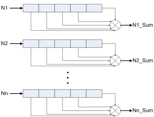
Figure 3.1: Block diagram of input window

The input window is a set ofnfive byte shift registers and a five input adder, as shown

in figure 3.1. Input to this component is an array of unsigned 8 bit integers indicating how

many spikes have occurred in each neuron since the input window was last clocked. When

the input window is clocked each shift register captures its corresponding input and shifts

all previous data by one, eliminating the oldest value. The contents of each shift register

are summed and that sum, another unsigned eight bit integer, is sent to the classifier stage.

If this stage is clocked at 50Hz it will effectively create a 100ms window that slides every

would be accumulated by an asynchronous counter that would be reset by the controlling

clock.

3.5

Classifiers

Figure 3.2: Block diagram of linear classifiers

Each classifier consists ofnmultipliers and one n input adder. Each multiplier,

imple-mented as a lookup table, takes one of the summed inputs provided by the input window

and converts it to a 32 bit signed integer based on the constant weight specific to that

clas-sifier and input. The n input adder, implemented as a linear array of two input adders, sums

the 32 bit integers produced by the multipliers. A total of m+ 1 classifiers were

particular movement type. A block diagram of the classifiers is shown in figure 3.2. Note

that this functionality consists solely of combinational logic, so no clock is necessary.

3.6

Output Logic

Figure 3.3: Block diagram of gating logic

The output decision logic consists of gating logic and movement logic, as in the

modi-fied algorithm described above. The gating logic takes input from the gating classifier and

determines if movement has or has not occurred. The movement logic takes input from

themmovement classifiers and determines the index of the largest movement value. Note

that since the multipliers used in the classifiers use weights scaled by α the output logic

constants must also be scaled byα.

The output of the gating classifier is sent to a three value 32 bit shift register that holds

t