Spectral modification of laser-accelerated proton beams by self-generated magnetic fields

(1)

T h e o p e n – a c c e s s j o u r n a l f o r p h y s i c s

New Journal of Physics

Spectral modification of laser-accelerated proton

beams by self-generated magnetic fields

A P L Robinson1,6, P Foster1, D Adams2, D C Carroll3, B Dromey2, S Hawkes1, S Kar2, Y T Li4, K Markey2, P McKenna3, C Spindloe1, M Streeter1, C-G Wahlström5, M H Xu4, M Zepf2 and D Neely1

1_{Central Laser Facility, STFC Rutherford-Appleton Laboratory, Chilton,}

Didcot, Oxfordshire, OX11 0QX, UK

2_{Department of Physics and Astronomy, Queens University Belfast,}

BT7 1NN, UK

3_{SUPA, Department of Physics, University of Strathclyde, Glasgow,}

G4 0NG, UK

4_{Beijing National Laboratory for Condensed Matter Physics, Institute of}

Physics, CAS, Beijing 100080, People’s Republic of China

5_{Department of Physics, Lund University, PO Box 118, S-221 00 Lund,}

Sweden

E-mail:alex.robinson@stfc.ac.uk

New Journal of Physics11(2009) 083018 (15pp)

Received 19 May 2009 Published 13 August 2009 Online athttp://www.njp.org/ doi:10.1088/1367-2630/11/8/083018

Abstract. Target normal measurements of proton energy spectra from ultra-thin (50–200 nm) planar foil targets irradiated by 1019_{W cm}−2_{40 fs laser pulses}

exhibit broad maxima that are not present in the energy spectra from micron thickness targets (6µm). The proton flux in the peak is considerably greater than the proton flux observed in the same energy range in thicker targets. Numerical modelling of the experiment indicates that this spectral modification in thin targets is caused by magnetic fields that grow at the rear of the target during the laser–target interaction.

6_{Author to whom any correspondence should be addressed.}

(2)

Contents

1. Introduction 2

2. Experimental set-up 3

3. Experimental results 4

4. Interpretation 5

5. Modification of spectrum by magnetic field 10

6. Conclusions 14

Acknowledgments 14

References 14

1. Introduction

The field of laser-driven ion acceleration from solid targets has developed rapidly since the development of chirped pulse amplification (CPA) lasers, which can now achieve intensities up to 1022_{W cm}−2_{. Activity in this area is being driven by the possibility of developing a}

radical alternative ion acceleration technology that might find application areas such as ion beam treatment of tumours, and ion-driven fast ignition inertial confinement fusion (ICF).

Most experiments have attributed the emission of multi-MeV proton and ion beams from solid targets irradiated at these intensities to the target normal sheath acceleration (TNSA) mechanism [1, 2]. The radiation pressure acceleration (RPA) mechanism may become very important in experiments that utilize intensities above 1021W cm−2 [3]–[5]. A number of experimental and theoretical studies have looked at a wide range of issues including energy scaling [6,7], beam collimation and focusing [8]–[10], beam control [11], conversion efficiency and flux [12,13] and control of the energy spectrum [14]–[16], especially in the context of the TNSA mechanism.

The development of simple methods of controlling and manipulating the ion energy spectrum has proved difficult. Those methods of generating quasi-monoenergetic spectra which have been demonstrated experimentally, have thus far required strong target cleaning [14]–[16], demanding target fabrication [14], or a secondary device [8, 9]. Therefore there is a strong motivation for finding simple laser–target configurations that can produce narrow-band ion energy spectra.

(3)

B-field is a common feature in particle-in-cell (PIC) simulations; however the existence of a proton-focusing region of the B-field is a novel feature for these experimental parameters. This produces a broad spectral peak in the target normal spectrum. The measured signal at the peak is much higher than it is in the thicker target spectra at the same energy—the spectral modification also enhances the proton flux. Theoretical studies of underdense targets at higher intensities (I _≈1022W cm−2) have indicated that proton-focusing B-fields can be formed [17, 18], although it has not been clear until now whether this could be realized or be significant at lower intensities (I _≈1019W cm−2) with planar solid foils. This is the first report of indications that there is a new regime of magnetically influenced TNSA in which highly non-Maxwellian spectra naturally occur.

Many experimental and theoretical studies of TNSA do not consider the effect of magnetic fields. However, a few publications have indicated that magnetic fields can be important [19,20] or at least have some role [21,22]. These papers have either considered targets that have been so severely decompressed by the laser pre-pulse as to be nearly underdense, or targets that are initially underdense. In these interactions, the laser pulse propagates through the plasma and exits at the rear of the target. In the experiment reported here, the laser pulse does not propagate through the target, so the regime studied in this paper is quite different to that considered in [19]–[22]. Furthermore, these previous experiments did not observe the spectral modifications that are described here. It must also be noted that these are target normal measurements—we arenot observing ‘monoenergetic rings’ as have been seen in previous experiments [23]–[25]. It is important to note that, unlike the interpretation given in [23, 24] where resistive B-field generation inside the target is important, the magnetic fields in the interpretation of these results are generated in a non-resistive fashion in the plasma expansion. As previously mentioned, theoretical studies of interactions with underdense targets and curved solid foils at significantly higher intensities (I _≈1022_{W cm}−2_{) than those considered here (}_I

≈1019_{W cm}−2_{) indicate that}

magnetic fields, and particularly proton-focusing regions of magnetic fields, can be important.

2. Experimental set-up

The experiment used the Rutherford-Appleton Laboratory’s ASTRA laser system. ASTRA is a Ti:sapphire laser that produces pulses with a 40 fs full-width at half-maximum (FWHM) duration that contain up to 700 mJ of energy. A plasma mirror set-up was used to improve the pulse contrast from 106at 1 ns to 108. In this set-up, the beam was focused onto an anti-reflection coated glass substrate and then re-collimated using two f/8 off-axis parabolas. The beam was finally focused onto a target at an incidence angle of 66.5◦_{using an f}/_{3 off-axis parabola. This}

produced a focal spot with an FWHM of 4–6µm at best focus.

The energy spectrum of the protons emitted into the forward direction was measured using an on-axis Thomson parabola spectrometer. This spectrometer detected protons by means of a scintillator that was optically coupled to an EMCCD7_{. This provided ‘on-line’, instantaneous}

spectra over a range of 0.2–6 MeV. The spectrometer was placed 532 mm from the target. Protons were admitted through a rectangular pin-hole that was 561×668µm. The scintillator detector was placed an additional 271 mm behind the pin-hole. The spectrometer had an energy resolution of 0.1 MeV at 1 MeV. Cross-calibration with CR-39 was performed to confirm the linearity of the detector. The targets used in this experiment were Al and plastic (CH) foils of 50 nm, 200 nm and 6µm thickness.

(4)

0 1 2 3 4 5 6 0

0.5 1.0 1.5 2.0 2.5 3.0x 10

4

0 1 2 3 4

0 2000 4000 6000 8000 10 000

0 1 2 3 4 5 6

0 2000 4000 6000 8000 10 000 12 000 14 000 16 000

Energy (MeV)

Proton energy spectrum (arb. units)

0 1 2 3 4 5 6

0 2000 4000 6000 8000 10 000 12 000

(a) (b)

[image:4.595.158.532.105.483.2]

(c) (d)

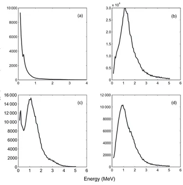
Figure 1.Proton energy spectra obtained from Thomson parabola spectrometer: (a) typical spectrum from a 6µm target, (b) spectrum obtained from 50 nm Al target with type I peak, (c) spectrum obtained from 50 nm CH target with type II peak and (d) spectrum obtained from 200 nm Al target with type I peak.

3. Experimental results

The functional form of the proton energy spectra from 6µm foil targets (either CH or Al) did not differ significantly from similar experiments on other laser systems, e.g. those reported in [13]. The spectra were quasi-exponential; figure 1(a) shows a typical spectrum. Quasi-exponential spectra are ubiquitous in laser-driven proton acceleration (see [26,27] for recent examples).

(5)

0 1 2 3 4 0

0.5 1.0 1.5 2.0x 10

4

0 1 2 3 4 0

0.5 1.0 1.5 2.0x 10

4

0 1 2 3 4 0

0.5 1.0 1.5 2.0x 10

4

0 1 2 3 4 0

0.5 1.0 1.5 2.0x 10

4

0 1 2 3 4 0

0.5 1.0 1.5 2.0x 10

4

0 1 2 3 4 0

0.5 1.0 1.5 2.0x 10

4

Energy (MeV)

[image:5.595.79.531.83.377.2]

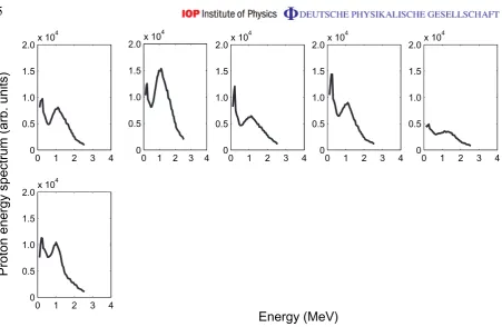
Figure 2.Proton energy spectra obtained from Thomson parabola spectrometer. Top row: the five spectra obtained from 50 nm CH targets that exhibited a type II peak. Bottom row: the single spectrum obtained from a 50 nm Al target that exhibited a type II spectrum.

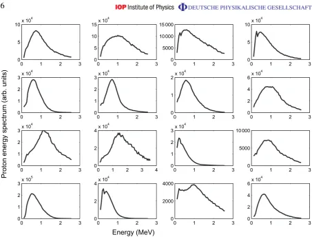
As figures1(b) and (c) show, there are two general types of spectral peak. The first type is where the spectrum falls on going from the peak to the low energy limit (16 shots; denoted as type I). The second type is where the spectrum initially falls and then rises again on going from the peak to the low energy limit (6 shots; denoted as type II).

The average position of the type I peaks is 0.7±0.3 MeV. The average position of the type II peaks is 1.1±0.1 MeV. On taking the average FWHM of the type I peaks, one obtains 1.1±0.4 MeV. All of the CH targets (5 shots) produced type II spectra, whereas all but one of the Al targets produced type I spectra. For clarity, the full range of the data obtained is also presented in this paper. In figure2, all six spectra that exhibited a type II peak are shown, and in figure3all 16 spectra that exhibited a type I peak are shown. Note that the ion signal at the energy of the peak is much higher than the signal measured at the same energy from the thicker targets. Therefore this spectral modification also results in enhancing the flux in certain energy ranges.

The slight variation in the spectra (e.g. the position of the single peak in the type I spectra) from shot to shot was attributed to the two aspects of the experiment which were the most difficult to stringently control: the intensity distribution in the laser focal spot and the laminarity/rugosity of the ultra-thin foils.

4. Interpretation

(6)

0 1 2 3 0

5 10x 10

4

0 1 2 3

0 5 10 15x 10

4

0 1 2 3

0 5000 10 000 15 000

0 1 2 3

0 5 10x 10

4

0 1 2 3

0 1 2 3x 10

4

0 1 2 3

0 1 2 3x 10

4

0 1 2 3

0 1 2x 10

4

0 1 2 3

0 2 4 6x 10

4

0 1 2 3

0 1 2 3x 10

4

0 1 2 3 4

0 2 4x 10

4

0 1 2 3

0 1 2 3x 10

4

0 1 2 3

0 5000 10 000

0 1 2 3

0 1 2 3x 10

5

0 1 2 3

0 2 4x 10

4

0 1 2 3

0 2000 4000

0 1 2 3

0 2 4 6x 10

4

[image:6.595.75.529.85.429.2]

Energy (MeV)

Figure 3.Proton energy spectra obtained from Thomson parabola spectrometer: all 16 shots from 50 nm Al targets that produced type I spectra.

spatial size of the proton source [14, 15] can be eliminated as the uncleaned foils would have formed contaminant layers of similar thickness irrespective of the actual foil thickness and these contaminant layers would cover the entire foil. As the composition of the contaminant layers was not controlled, and typically the relative proton fraction would be high, the ‘two species mechanism’ [28]–[30] is unlikely to account for the spectral peak, and would not account for the dependence on target thickness. The ‘two species mechanism’ has been used to explain some experimental results, notably those by Allen et al[31]; however, an important reason why the ‘two species mechanism’ is unable to explain these results is that no such spectral modulations were observed in the 6µm targets. Another possibility is that the spectral peak is formed by the contribution of protons that are accelerated at the front of the target by the light pressure of the laser pulse [3]–[5], [32]. The energy of ions produced byhole-boringRPA is given by,

ε=mic2

24

1 + 2√4

, (1)

where4=I/ρc3[33]. At I ₌1019W cm−2andρ≈1000 kg m−3 (water or oil contaminants),

ε≈7 keV. Therefore front surface acceleration cannot account for this spectral peak, in agreement with previous experimental work [34].

(7)

0 1 2 3 4 0

100 200 300 400 500 600

0 1 2 3 4

0 50 100 150 200 250 300

0 1 2 3 4

0 1 2 3 4 5x 10

4

0 1 2 3 4

0 2 4 6 8 10 12x 10

4

Energy (MeV)

(a) (b)

[image:7.595.162.530.89.417.2]

(c) (d)

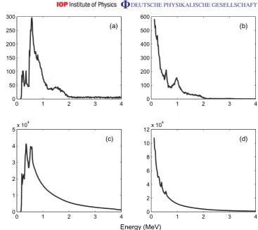
Figure 4.Proton energy spectra from 2D PIC simulations at 200 fs: (a) spectrum from 80 nm ‘Al’ foil simulation of protons travelling at <0.5 mrad to target normal, (b) spectrum from 80 nm ‘CH’ foil simulation of protons travelling at

<0.5 mrad to target normal, (c) spectrum from 80 nm ‘Al’ foil simulation of all protons and (d) spectrum from 80 nm ‘CH’ foil of all protons.

OSIRIS [35]. The simulation box was 30µm longitudinally (x) and 20µm in the transverse (y) direction. In the transverse direction, 10 000 cells were used, and 16 000 cells were used in the longitudinal direction. Given the limitation in computational resources the following models were used: the CH targets were modelled by a target consisting of H+ at a density of 80ncrit and D+ (as a ‘heavy’ ion species) at a density of 40ncrit.8 The Al targets were modelled

by a target consisting of D+ at a density of 120ncrit, with a 10 nm thick proton bearing layer

with same composition as the ‘CH’ target on the rear of the target. Electrons and protons were represented by 256 macroparticles per cell, and heavy ions were represented by 128 macroparticles per cell. The target was 80 nm thick, 10µm wide and was located 6.05µm from the left-hand boundary. The laser pulse propagated along the +x-direction from the left-hand boundary and was normally incident. The pulse had a 40 fs FWHM duration, a FWHM intensity of 2.2×1019_{W cm}−2_{, and a FWHM spot diameter of 4}_.₄_µ_{m. The simulation was run}

up to 250 fs. Another simulation was also carried out with a ‘CH’ target that was 1µm thick. When the proton energy spectra of both targets were calculated using all protons, the agreement with experiment was poor—see figures 4(c) and (d). The ‘CH’ target spectrum was

8 _n

(8)

monotonically falling with no strong spectral features. The ‘Al’ target spectrum produced two peaks instead of a single peak. It was therefore decided to calculate the energy spectra in a way that better represented the actual spectrometer—the spectrum was calculated using only those protons travelling at an angle of 0.5 mrad to the target normal. The ‘angularly filtered’ (i.e.<0.5 mrad) spectra were quite different. In figure4(a), the filtered proton energy spectrum for the ‘Al’ target is shown, and that of the ‘CH’ target is shown in figure4(b). This agrees very well with the experimental results. In the case of the 1µm thick ‘CH’ target, the spectrum was exponential irrespective of angular filtering. In the 80 nm ‘CH’ simulation, the spectral peak sits at 0.98 MeV and the form of the spectrum is very much like the type II spectra. In the ‘Al’ simulation, the spectral peak sits at 0.58 MeV, and the form of the spectrum is very much like the type I spectra. There is therefore good qualitative and quantitative agreement between these simulations and the experiments.

A detail examination of the simulation results showed that the front surface acceleration was negligible as expected. The effect of the heavy ions in the ‘CH’ simulation is also negligible. Only when one examines only those protons that are very close to the target axis does one find that the heavy ions generate a small modulation at 0.5 MeV, but when one integrates over all protons (with or without angular filtering) this modulation is smeared out. This means that, for these conditions, the PIC simulations indicate that the ‘two species mechanism’ used by Allenet al[31] does not play a significant role in these observations.

On the basis of these simulation results it was concluded that the spectral modification was dominated by an effect that caused angular deflection of the protons. There are two possible causes—a transverse electric field or an azimuthal magnetic field. If it is an electric field, then, over 200 fs (i.e. a distance of 2µm), a 500 keV proton would have to experience an average electric field of 109_{V m}−1 _{to be deflected by 1 mrad. If it is a magnetic field then, over 200 fs,}

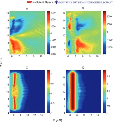
a 500 keV proton would have to experience an average magnetic flux density of ≈50 T. On examining the PIC simulation output, it was found that the Ey component of the E-field was negligible. TheBzcomponent of the B-field was not. A quasi-static B-field with flux densities in excess of 1000 T develops at the back of the target. The extent of this region is several microns in yand 1–2µm inx. This is shown in figure5(a), for the case of the 80 nm ‘CH’ target simulation. This is more than sufficient to strongly deflect protons away from the target normal (20 mrad in 200 fs).

The generation of this strong magnetic field emerges from the transverse spatial profile of the sheath field at the back of the target. From the induction equation, B˙ _{= −∇ ×}E, one can estimate the growth rate at early times to be ˙Bz_≈√nfkBTf/ε0/rf, where nf is the fast

electron density, Tf the fast electron temperature andrf the fast electron beam radius. In very

thin targets, r_f will be close to the laser spot radius. For typical parameters (n_f_≈1027_m−3_,

T_f_≈1 MeV,r_f_≈5µm), one obtains a growth rate of the order of 1017_–1018_{T s}−1_{. This means}

that magnetic fields of the order of 1000 T will grow in tens of femtoseconds. The generation of strong magnetic fields occurs for both thick and thin targets.

(9)

[image:9.595.152.533.88.497.2]

Figure 5. Plots of magnetic flux density, Bz(T), in simulation of 80 nm ‘CH’ target (a) and 1µm (b) at 200 fs. Plots of proton density (log₁₀(n_p/n_crit)) in simulation of 80 nm ‘CH’ target (c) and 1µm (d) at 200 fs. Foil is initially positioned atx ₌6.05µm. Note that a region whereBz>1000 T extends 1–2µm away from the rear surface.

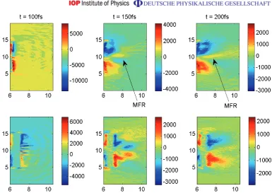
the target axis. The protons that are close to the mid-plane move through a region of focusing magnetic field (between 7 and 8µm as figure5(a) shows). The temporal evolution of this region of focusing magnetic field is shown in figure 6 in which we show the Bz component of the magnetic field in the 80 nm ‘CH’ simulation at 100, 150 and 200 fs, and we indicate the focusing region. The same plots for the 1µm ‘CH’ simulation are also shown to show the absence of any focusing region.

The generation of this focusing region can be at least partly explained by considering E

(10)

[image:10.595.145.531.91.364.2]

Figure 6.Top row: plots of magnetic flux density, Bz(T), in simulation of 80 nm ‘CH’ target at various times (100, 150 and 200 fs) showing the evolution of the region of magnetic field that can focus the protons. The focusing region is indicated by the label ‘MFR’. Bottom row: plots of magnetic flux density,Bz(T), in simulation of 1µm ‘CH’ target at various times (100, 150 and 200 fs). Note the clear absence of a focusing region in the 1µm simulation.

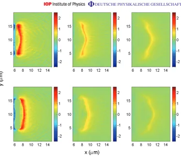
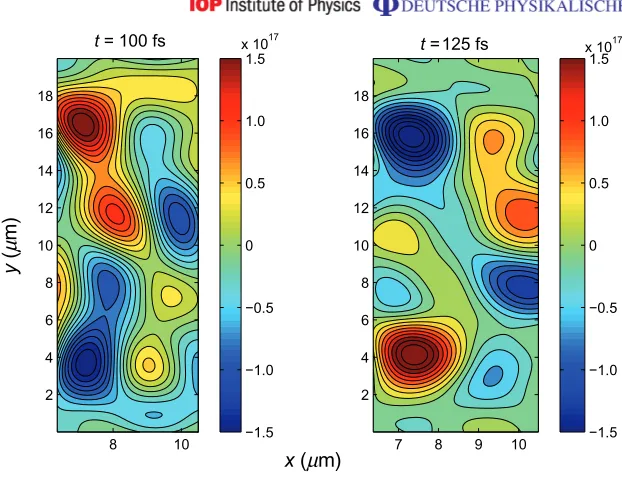
by figure7. In the case of the simulation of the 80 nm target it was found that theEx sheath field was strongest in a thin linear region parallel to the target surface which is slightly bowed at the centre. This bowing leads to a transverse variation in Ex which changes|∇ ×E| and thus the growth rate of the magnetic field. In contrast the simulation of the 1µm target shows that the Ex profile is less bowed at early times (100 fs), and the magnitude of the sheath field decays more rapidly. Figure6indicates that the most important time for the magnetic field growth is between 100 and 150 fs. Examining−∇ ×Ebetween these times shows how the changing electric field structure is actually generating the magnetic field. This is shown in figure89in which we show −∇ ×Eat 100 and 125 fs in the 80 nm ‘CH’ simulation to illustrate how this field structure leads to the generation of a focusing region. Figure8shows that in this 25 fs period there is a region of sustained growth of a focusing B-field, and it is this that gives rise to the focusing region seen in figure6. Note how the magnetic field growth rate compares to the simple order-of-magnitude estimate.

5. Modification of spectrum by magnetic field

The majority of the magnetic field in both simulations acts to defocus the proton beam; however, the analysis of the proton spectrum for various degrees of angular filtering indicate that the

9 _{For these plots, filtering via Fourier transform methods has been used to eliminate high-frequency noise in the}

(11)

[image:11.595.152.527.87.409.2]

Figure 7.Top row: plots of Ex (TV m−1) in the 80 nm ‘CH’ target simulation at different times. Left–right: at 100, 125 and 150 fs. Bottom row: plots of Ex in the 1µm ‘CH’ target simulation at different times. Left–right: at 100, 125 and 150 fs. Note how the sheath field is strongest in a thin strip that runs parallel to the target surface and is slightly bowed at the centre.

degree of spectral modification that this causes is minimal. This is why the full spectrum from the 1µm target simulations differs little from the angularly filtered spectrum. Largely this is not unexpected as the defocusing magnetic field is strongest far from the target normal axis where proton flux is low. However, the focusing region of the magnetic field that is observed in the thin target simulations sits close to the target normal axis where the proton flux is strong.

The presence of a region of focusing magnetic field can modify the energy spectrum in a similar way to the effect observed in the laser-driven micro-lens [8]. The angular deflection of a proton is the product of its ‘dwell time’ in the B-field and the gyro-frequency of the field, i.e.

1θ =ωg,pτ. This can be put in the following form:

1θ = e Bτ

mp

, (2)

(12)

x (µm)

y

(

µ

m)

t = 100 fs

8 10 2 4 6 8 10 12 14 16 18 −1.5 −1.0 −0.5 0 0.5 1.0 1.5

x 1017 t = 125 fs

[image:12.595.148.459.93.333.2]

7 8 9 10 2 4 6 8 10 12 14 16 18 −1.5 −1.0 −0.5 0 0.5 1.0 1.5 x 1017

Figure 8. Plots of B˙ _{= −∇ ×}E at 100 fs (left) and 125 fs (right) in the 80 nm ‘CH’ simulation. This shows that during this period there is sustained growth of a proton-focusing B-field near the target axis between 7 and 8µm in x, and between 6 and 12µm in y.

must be for protons of an intermediate energy. Spectral modification can therefore occur and be determined by the variation in dwell time with proton energy. Note that the finite spatial extent of the focusing region also implies that the highest energy protons are unlikely to have the longest dwell times.

This can be illustrated via a simple model calculation. Suppose that we have a proton beam with the following momentum distribution function:

f _∝exp

− p

2

x 2Tx

exp − p

2

y

2Ty !

, (3)

where pis normalized tom_pc, andT is normalized tom_pc2_{. The effect of propagation through}

a focusing magnetic field (in the z-direction) is to perform two rotations on each two separate distributions each containing half the number of particles in px–py phase space separately. Two rotations are done assuming that an equal number of protons enter each lobe of the focusing B-field. The angle of rotation is determined by equation (2). Since the rotation is only a function of energy, this transforms the distribution function by,

f(px,py)_→ f(pxcos1θ+ pysin1θ,pycos1θ₋pxsin1θ), (4)

for py >0. For py<0, the same transformation is applied but with−1θ. Once both rotations are done, the two are added to recover the full distribution function. For the dwell time,τ, we will use the following expression which is purely a model expression that gives a peak dwell time at intermediate energy,

τ =(5×10−14)sin(πε/1.5Tx)s, (5)

(13)

0.01 0.02 0.03 0.04 0.05 0.06 −2.5

−2.0 −1.5 −1.0 −0.5 0 0.5 1.0 1.5 2.0 2.5

−2.5 −2.0 −1.5 −1.0 −0.5 0 0.5 1.0 1.5 2.0 2.5 x 10−3

p x / mpc p y

/

m p

c

0.01 0.02 0.03 0.04 0.05 0.06

x 10−3 D

[image:13.595.149.529.105.320.2]

I

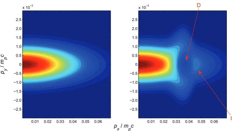
Figure 9. Results of simple model calculation to demonstrate effect of spectral modification by magnetic fields (see section5). Left hand figure is a px–py plot of the initial proton distribution. Right hand figure is a px–py plot of the proton distribution after rotations have been performed. The depression in the modified distribution is indicated by the label D, and the ‘island’ in the distribution that will produce a spectral peak is labelled I.

In figure 9, we plot the initial distribution function given by equation (3), the distribution function after being transformed by the magnetic field. For these calculations, Tx =0.0008 (0.75 MeV), Ty =4×10−7 (38 keV), and B=1500 T, which are representative of the proton emission close to the target axis in the 2D PIC simulations. The simple model calculation shows that a small ‘island’ is formed in the px–py phase space with a depression just to the left of it. This ‘island’ will lead to a spectral peak if the spectrum is only measured over a limited angle. The depression is formed by over-focusing of the protons at those energies where the dwell time is largest.

(14)

[image:14.595.147.418.91.327.2]

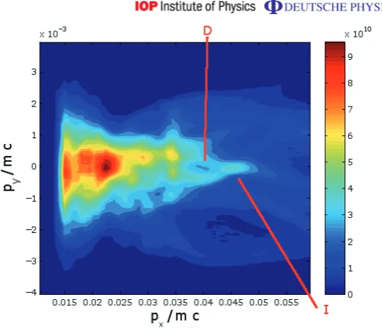
Figure 10.The px–py phase space distribution of the protons from the 2D PIC simulation of the ‘CH’ target at 200 fs. The ‘island’ feature, which produces the spectral peak is labelled I and sits close to px =0.045, i.e. 0.95 MeV.

6. Conclusions

In conclusion, proton beams from ultra-thin (50–200 nm) foils irradiated by a 1019_{W cm}−2_,

40 fs laser pulse were found to have energy spectra that contained a broad peak near to 1 MeV. By carrying out 2D PIC simulations of the experiment, it has been concluded that quasi-static magnetic fields at the rear of the target are responsible for producing these spectral peaks. As the spectrometer only measures those protons that are emitted into a narrow cone, the quasi-static magnetic field will strongly shape the spectrum by deflections in the field that are dependent on the dwell time of the proton in the field. This produces broad spectral peaks. This may provide a new or complementary route to optically controlling the energy spectrum of laser-accelerated proton beams, in contrast to the ‘target engineering’ approach, which has previously been advocated [14]. This work also highlights a more generic issue—that of properly accounting for the limited angular sampling of magnetic spectrometers when interpreting ion acceleration experiments.

Acknowledgments

We are grateful for the use of computing resources provided by Science and Technology Facilities Council’s e-Science facility. We are also grateful for the support of EPSRC (grant no. EP/E048668/1) and the NSFC (grant no. 10720101075).

References

[1] Wilks S Cet al2001Phys. Plasmas8542

[2] Mora P 2003Phys. Rev. Lett.90185002

(15)

[4] Macchi Aet al2005Phys. Rev. Lett.94165003

[5] Robinson A P Let al2008New J. Phys.10013021

[6] Fuchs Jet al2006Nat. Phys.248

[7] Robson Let al2007Nat. Phys.358

[8] Toncian Tet al2006Science312410

[9] Kar Set al2008Phys. Rev. Lett.100105004

[10] Schollmeier Met al2008Phys. Rev. Lett.101055004

[11] Carroll Det al2007Phys. Rev.E76065401