Communicability in complex networks

Communicability in complex networks

Ernesto Estrada1* & Naomichi Hatano2

1

Complex Systems Research Group, X-rays Unit, RIAIDT, Edificio CACTUS, University of Santiago de Compostela, 15076 Santiago de Compostela, Spain

2

Institute of Industrial Science, University of Tokyo, Komaba 4-6-1, Meguro, Tokyo 153-8505, Japan

*

We propose a new measure of the communicability of a complex network, which is a broad generalization of the concept of the shortest path. According to the new measure, most of real-world networks display the largest communicability between the most connected (popular) nodes of the network (assortative communicability). There are also several networks with the disassortative communicability, where the most “popular” nodes communicate very poorly to each other. Using this information we classify a diverse set of real-world complex systems into a small number of universality classes based on their structure-dynamic correlation. In addition, the new communicability measure is able to distinguish finer structures of networks, such as communities into which a network is divided. A community is unambiguously defined here as a set of nodes displaying larger communicability among them than to the rest of nodes in the network.

I. INTRODUCTION

Complex networks represent interactions between pairs of units in disparate physical, biological, technological and social systems [1-4]. A focus of research in this field is the search of good measures, global or local, that quantify unique characteristics of the networks [5-7]. Most of the measures currently in use are based on the shortest paths connecting two units (nodes) of a network [5-7]. Their relevance rests on the premise that communication between the nodes takes place through the shortest paths [8-10].

At a local scale, the shortest path is often used to identify network communities [11, 12] or to characterize the importance of the nodes in a network [13]. For instance, the boundaries of a community are commonly defined [11] on the basis of the influence of a node over the flow of information between other nodes, assuming that this flow primarily follows the shortest paths. At a global scale, the use of many concepts like the average shortest path length [14], the degree-degree correlations [15] and the degree distribution [16] emphasizes the “communicability” through the shortest paths. Communicability must be understood here as capable of being easily communicated or transmitted in terms of passage or means of passage between the different nodes in a network.

However, “information” can in fact spread along non-shortest paths [14, 17]. We can think, for instance, of gossip spreading in a social network, where the information can flow back and forward several times before reaching the final destination. Consequently, concepts like “small worldness” [18], “assortativeness” [19] or “scale-freeness” [16] can miss important information on the network communicability as well as on finer structures of the network depending on it [20].

II. COMMUNICABILITY IN COMPLEX NETWORKS

A. Definition

We consider networks represented by simple graphs G=

(

V,E

)

, that is, graphs having V =n nodes and E =m links, without self-loops or multiple links between nodes. Let A

( )

G = A be the adjacency matrix of the graph whose elements A_ij are ones or zeroes if the corresponding nodes i and j are adjacent or not, respectively. We call the eigenvalues of the adjacency matrix in the non-increasing order λ1 ≥λ2 ≥m≥λ_n,

the spectrum of the graph [21].

It is well-known that the

(

p,q

)

-entry of the kth power of the adjacency matrix,

Ak

( )

pq, gives the number of walks of length k starting at the node p and ending at the

node q [21]. A walk of length k is a sequence of (not necessarily different) vertices k

k v

v v

v₀, ₁,_m, ₋₁, such that for each i=1,2_m,k there is a link from v_i−1 to v_i . Consequently, these walks communicating two nodes in the network can revisit nodes and links several times along the way, which is sometimes called “backtracking walks”. In contrast, a path is a sequence of different vertices.

The communicability between a pair of nodes in a network is usually considered as the shortest path connecting both nodes. We now propose a generalization of the communicability by accounting not only for the shortest paths communicating the nodesp and q but also for all the other walks that permit for a “particle” to travel from one to the other.

The theoretical justification for this consideration is two-fold. First, it is known that communication between a pair of nodes in a network does not always take place through the shortest paths but it can follow non-shortest paths. The other justification is that the shortest paths are not very sensitive with respect to the appearance of structural bottlenecks in a network. On the contrary, the number of walks is significantly affected by the appearance of such structural changes in a network.

Our strategy here is to make longer walks have lower contributions to the communicability function than shorter ones. If P_pq(s)

is the number of the shortest paths between the nodes p and q having length s and W_pq(k)

is the number of walks connecting p and q of length k >s, we propose to consider the quantity

G_pq = 1

s!Ppq + 1

k!Wpq

(k)

k>s

∑

. (1)

the node p. As some of these “detours” can be very long, the summation is weighted in decreasing order of the length of the walk.

Using the connection between the powers of the adjacency matrix and the number of walks in the network, we obtain

( )

_{( )}

∑

∞ = = = 0 ! k pq pq k pq e k

G A A . (2)

This can be further rewritten in terms of the graph spectrum as [22]

G_pq = ϕj

( )

p ϕj

( )

q j=1

n

∑

eλj _{, (3)}

where ϕj

( )

p is the pth element of the jth orthonormal eigenvector of the adjacency matrix associated with the eigenvalue λ_j [21]. We call G_pq the communicability

between the nodes p and q in the network.

B. Bounds

Intuitively, the communicability should be minimal between the end nodes of a linear chain. In fact, the communicability between the end nodes of a chain vanishes as the length of the chain is increased. The oscillation of one end dies out before it reaches the other end. On the other hand, if we consider a complete graph, where every node is connected to all other nodes, the Green’s function between an arbitrary pair of nodes diverges as the size of the graph is increased. The oscillation is greatly amplified because of the infinitely many walks between the nodes. Thus, the communicability between a pair of nodes in a network is bounded between zero and infinity, which are obtained for the two end nodes of an infinite linear chain and for a pair of nodes in an infinite complete graph.

This intuition can be proved mathematically as follows. It is known that the eigenvalues and eigenvectors of a linear chain of n nodesP_n are given by the following expressions [23]:

λj =2 cos

jπ

n+1  



 and ϕj

( )

p = 2

n+1sin

pjπ

n+1

 



 . (4)

Then the value of G_pq for the chain P_nis equal to

Gpq = 1

n+1 cos

jπ

(

p−q

)

n+1 −cos

jπ

(

p+q

)

n+1 



 e

2 cos jπ

n+1     j

∑

. (5)

Let P_∞ be a chain of infinite length. It is straightforward to realize by simple substitution in (5) that G_1,∞ =0 for the end nodes p=1 and q= ∞.

Because the eigenvectors are orthonormalized we can represent them as the columns of an orthogonal matrix Q. Then, by the properties of an orthogonal matrix we have that

I QQ Q

QT = T = _{. The second part of this expression means that the product of any two}

rows of Q is equal to zero, which can be written as,

( ) ( )

0

1 =

∑

= q p _j n j j ϕ ϕ .

Then, because ₁ 1

(

1 _m 1

)

n

=

ϕ , is the normalized eigenvector associated to

the eigenvalue n−1 , the previous equality immediately implies that

( ) ( )

n q p _j n j j 1 2 − =

∑

= ϕ

ϕ . We hence obtain

G_pq = e

n−1

n +e

−1 _ϕ

j(p)ϕj(q)= j=2

n

∑

e

n−1

n − 1 ne = 1 ne e n −1

(

)

. (6)

It is easy to see that G_pq → ∞ as n→ ∞ for K_n.

III. COMMUNICABILITY AS THE GREEN’S FUNCTION OF

NETWORKS

We now argue that the communicability defined above is actually the Green’s function of the network. For a given network with the adjacency matrix A, imagine the following system. We have a spring on each link of the network. We somehow put the network of springs on a plane, adjusting the natural length of the springs so that the system may be at rest on the plane. Each node can oscillate in the direction perpendicular to the plane. The pth node, when at height zp, feels the force

K

(

z_p−z_q

)

q

∑

A_pq, where K is the common spring constant, because the pth node is

connected by a spring to the qth node only if A_pq =1. We also add a special spring connecting each node to the ground, creating a force −2Kk_pz_p, where kp is the degree of

the pth node, or the number of links attached to the pth node. In other words, the potential energy for the pth node is given by

Up =

K

2 q

(

zp −zq

)

∑

2Apq −Kkpzp

2

(7)

and hence the total energy is given by

E= Up

p

∑

= K

2 p,q

(

zp −zq

)

∑

2Apq−K kpzp

2

p

∑

, (8)

which after some algebraic manipulation is transformed to the expression

E= −K z_pA_pqz_q

p,q

∑

. (9)

Z= e−βE

all configurations

∑

= exp βK z_pA_pqz_q

p,q

∑

     

∫

dz_q

q

∏

. (10)

We can transform the partition function in terms of the normal modes. Suppose that we diagonalize the adjacency matrix A in the form A_pqϕj(q)

q

∑

=λjϕj(p) . Then the

partition function (10) is transformed to

Z= exp βK λjuj

2 j

∑

     

∫

du_j

j

∏

, (11)

where u_j = z_qϕj(q) q

∑

. The integration in (11) is now possible, being the product of

Gaussian integrals.

Let us now calculate the correlation function, or the (thermal) Green’s function

G_pq(β)= z_pz_q = 1

Z

∫

zpzqexp βK s,t zsAstzt

∑

 

  dzr

r

∏

. (12)

After the same transformation above, we obtain

G_pq(β)= z_pz_q = ϕj(p) j

∑

ϕj(q)e

βKλj ₌ β

k

k!Wpq

(k)

k≥s ∞

∑

. (13)

This describes how much the qth node oscillates when we shake the pth node.

In general, the Green’s function expresses how an impact propagates from one place to another place. In this sense, Eq. (13) is nothing but the Green’s function of the network. From another point of view, we can consider particle diffusion on the complex network. Then the Green’s function (13) describes how many particles end up at the qth node if we put particles at the pth node.

We can make another connection of the communicability to the Green’s function by considering a continuous-time quantum walk on the network. Take a quantum-mechanical wave function ψ

( )

t at time t. It obeys the Schrödinger equation [22]

( )

t

( )

t dt

d

i ψ =−Aψ _{, (14)}

where we use the adjacency matrix as the negative Hamiltonian.

Assuming from now on that =1 _{we can write down the solution of the}

time-dependent Schrödinger equation (14) in the form ψ

( )

i t ψ

( )

0

e t A

= . The final state

q eiAt

is a state of the graph that results after time t from the initial state q . The “particle” that resided on the node q at time t =0 diffuses for the time t because of the quantum dynamics. Then, we can obtain the amplitude that the “particle” ends up at the node p of the network by computing the product peiAt q

q e p G_pq A

= , which is the communicability between nodes p and q in the network as defined in this work. Consequently, the communicability between nodes p and q in the network represents the probability that a particle starting from the node p ends up at the node q after wandering on the complex network due to the thermal fluctuation. By regarding the thermal fluctuation as some forms of random noise, we can identify the particle as an information carrier in a society or a needle in a drug-user network.

IV. STRUCTURE-DYNAMICS RELATIONSHIPS

In order to investigate the structure-dynamics relationship in complex networks, we use the correlation between the node degree and the communicability (the Green’s function). The node degree k_p is one of the simplest topological characteristics of a network defined as the number of links attached to a node. The correlation can be observed in the form of three-dimensional contours where k_p and k_q form the x and y

axes, and G_pq is plotted as the z axis. We then fit the data points by using the weighted least square method, which is implemented in the STATISTICA package. This method is similar to the one proposed by McLain for drawing contours from arbitrary data points [24].

A. Structure characterization

A network can display a homogeneous distribution of the nodes in a way that two arbitrary regions of the network display similar organizational characteristics. Such a network is characterized by the lack of highly inter-connected regions or clusters separated from one another by a few nodes/links, which are known as bottlenecks. In Fig. 1 (left graphic) we illustrate a hypothetical network displaying structural homogeneity, where two different regions show similar topological characteristics when magnified. In these networks a plot of a property characterizing the local neighborhood around a node should scale perfectly to another property characterizing the global topology of the network. In other words, what you see locally is what you get globally. It is necessary to comment here that the lack of structural bottlenecks in a homogeneous network does not imply the lack of communities in such network. Thus, we can observe communities of highly interconnected nodes which are well-communicated from one another by a few links.

local and a global topological characterization of the network. that is, what you see locally is not what you get globally.

Insert Fig. 1 here.

B. Quantitative determination of network homogeneity

In order to determine whether a network is homogeneous we start by characterizing the neighborhood of a node by means of the subgraph centrality [25]. The subgraph centrality is defined as [25]

( )

[

( )

]

j

e i i C N j j

S _ϕ λ

2

1

∑

=

= (15)

Then, expressing the exponential in term of hyperbolic functions we can express the subgraph centrality as the sum of two terms characterizing the odd and even contributions [26]

( )

( )

( )

[

( )

]

( )

[

( )

]

( )

j

N j j j N j j even S odd S S i i i C i C i

C ϕ sinhλ ϕ coshλ

2 1 2 1

∑

∑

= = + = +

= (16)

It is straightforward to realize that we can write odd subgraph centrality in the following form:

( )

[

( )

]

( )

[

( )

]

( )

j

N j j odd S i i i

C ϕ sinh λ ϕ sinhλ

2 2 1 2 1

∑

= + = (17)

where λ₁ and ϕ₁ are the principal (Perron-Frobenius) eigenvalue and eigenvector of the network, respectively. This expression can be represented in a logarithmic scale in the following form (through the whole paper we will use base-10 logarithms designated as

10

log log= ):

( )

( )

[

( )

]

( )

[

( )

1

]

2

2

1 0.5log sinh 0.5logsinh

logϕ ϕ λ − λ

        − =

_∑

= j N j j odd

S_{C i i}

i (18)

This expression can be represented as a straight line in a plot of logϕ₁

( )

i versus

( )

[

]

( )

{

1

}

2

1 sinh

log ϕ i λ , with a slope of 0.5 and intercept of −0.5log

[

sinh

( )

λ₁

]

[27].

Now, let us consider a homogeneous network defined in the following way. A network is consider to be homogeneous if every subset S of nodes (S ≤ 50% of the nodes) has a neighborhood that is larger than some “expansion factor” φ multiplied by the number of nodes in S. A neighborhood of S is the set of nodes which are linked to the nodes in S [28]. Formally, for each vertex v∈V (where V is the set of nodes in the network), the neighborhood of v , denoted as Γ

( )

v is defined as:

( )

v =

{

u∈V

(

u v

)

∈E

}

Γ , (where E is the set of links in the network). Then, the neighborhood of a subset S ⊆V is defined as the union of the neighborhoods of the nodes in S:

( )

( )

S

v v

S

∈ Γ

=

definition of network homogeneity is in agreement with our intuitive idea illustrated in Fig. 1A. That is a network is homogeneous if what you “see” locally is what you get globally. These homogeneous graphs are known in the literature as good expanders.

It has been proved [28] that graphs with very large spectral gap λ >>₁ λ₂ are very good expanders. In this case it is easy to see that [27, 29]:

( )

[

]

( )

[

( )

]

( )

j N

j j i

i λ ϕ λ

ϕ sinh sinh

2 2 1 2 1

∑

=

>> (19)

and

( )

[

( )

]

( )

1 2

1 sinh λ

γ i i

C_odd

S _≈

. (20)

Consequently, those networks displaying homogeneous characteristics as defined by the good expansion character display a perfect spectral scaling between logϕ₁

( )

i and

( )

i C_odd

S

ln [27]:

( )

( )

[

( )

1

]

1 0.5log 0.5logsinh

logϕ i = SC_odd i − λ (21)

In summary, if we obtain a perfect straight line when plotting logϕ₁

( )

i versus

( )

[

]

( )

{

1

}

2

1 sinh

log ϕ i λ , with a slope of 0.5 and intercept of −0.5log

[

sinh

( )

λ₁

]

, the network has good expansion character and consequently it is homogeneous. If the plot displays a dispersion of points the corresponding network is not homogeneous. These two cases correspond to the hypothetical plots illustrated in Fig. 1. Then, the deviation from the perfect straight line ξ

( )

G in the spectral scaling plot can be considered as a quantitative measure of the homogeneity of a network. A perfectly homogeneous network will have ξ

( )

G =0; the higher the value of ξ

( )

G the larger the departure of the network from homogeneous properties [30]:

( )

∑

{

[

( )

]

[

[

( )

]

[

( )

]

]

}

= − + − = N i odd S i C i N G 1 2 5 . 0 1

1 logsinh 0.5log

log 1

λ ϕ

ξ (22)

B. Degree-communicability correlations

According to the degree-communicability pattern, networks can be classified in any of the following four theoretically possible classes:

Class (a): Non-homogeneous networks with assortative communicability; Class (b): Non-homogeneous networks with disassortative communicability; Class (c): Homogeneous networks with assortative communicability;

Class (d): Homogeneous networks with disassortative communicability.

communicability takes place among the hubs and the lowest communicability occurs between nodes of low degree.

We start by considering the first three possible types of networks according to their degree-communicability patterns, i.e., (a), (b) and (c). First, we build three possible toy network structures, which are shown in Fig. 2 together with their

k_p,k_q,G_pq

(

)

-plots for every pair of nodes (p,q) . These graphs are built for illustration

and are neither the result of an empirical search nor of a simulation. The node degree kp

denotes the number of the links attached to the node p.

Insert Fig. 2 here.

In Fig. 2a we illustrate a hypothetical network formed by two communities of nodes with high internal connectivity, which are separated by very few nodes/links. This network will display a non-homogenous structure due to the obvious presence of the node/links bottlenecks. In some situations, networks with bottlenecks can display AC. Two typical examples are a network where most of the hubs are located in one of the tightly connected clusters and a network where the hubs are the bottlenecks. In such cases as the one illustrated in Fig. 2a the networks will display non-homogeneous structure with assortative communicability between the nodes.

The contour plot in Fig. 2b might appear to be counterintuitive. In social networks terminology [13], it is equivalent to saying that the most popular people are poorly communicated among them. This situation emerges when there are a couple of leaders, each of whom forms a community of many followers. The communication between the communities can be bad, and hence there is poor communicability between the leaders. This example represents a hypothetical illustration of a non-homogeneous network with disassortative communicability between nodes.

The third contour plot in Fig. 2 fits intuitive interpretation; the communicability

Gpq is high between pairs of hubs, or nodes of high degree. AC can appear in very

homogeneous networks where the hubs can communicate to each other without structural bottlenecks (see Fig. 2c).

nodes. As a result there will be a large hub-hub communicability, which in any case is expected to be larger than the communicability between hubs and low-degree nodes. In summary, we conclude that it is not possible to build homogeneous networks with disassortative communicability between nodes. More work should be done in this direction, particularly for searching theoretical justification for this empirical observation.

C. Empirical analysis of real-world networks

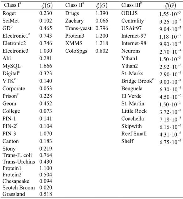
In this work we study 50 real-world networks of different sizes and types, e.g., informational, technological, social, biological and ecological [31]. Our empirical analysis of these networks shows that there is 52%, 12%, 36% and 0% of networks in each of four classes previously defined, respectively (see Table I where we also give the values of ξ

( )

G ). In Fig. 3 we show contour plots for some of these real-world networks: (a) the airport network in the USA; (b) the semantic network of the Roget’s thesaurus; (c) the food web of Bridge Brook; (d) the direct transcription network between genes of yeast (S. cereviciae); (e) the social network of injecting drug users (IDUs); (f) the social network of people with HIV infection in Colorado Spring during the period of 1985-1999 [31].

Insert Table I and Fig. 3 here.

The first two networks (Fig. 3a and b) clearly display AC. The USA airport network is characterized by the lack of topological bottlenecks [27]. This structural homogeneity results in the high inter-hub communicability of Class (c) as in Fig. 2c. The Roget’s thesaurus network also displays AC despite it is formed by several clusters separated by structural bottlenecks [27]. In this case, however, there is a preference of the hubs to be connected to other hubs, and hence we have Class (a) as in Fig. 2a.

The food web in Fig. 3c forms a homogeneous network without large structural bottlenecks [32]. However, this network shows very large preference of the hubs to be attached to low degree nodes. Consequently, most of the inter-hub communication takes place by indirect routes decreasing the inter-hub communicability.

interchange needles among them. This core is formed by several hubs, i.e., individuals that share their needles with a large number of other users. These hubs interchange their needles among them giving rise to certain AC characteristics observed in the contour plot of Fig. 3e. However, there are several other groups in the network lead by other individuals with large number of internal connections. These groups are almost isolated and communicate among them only through very few individuals. This gives rise to the DC characteristics observed in Fig. 3e. In the case of the risk network of Colorado Spring there is not a highly interconnected core [33] and the network shows very clear DC characteristics.

V. COMMUNICABILITY AND NETWORK COMMUNITIES

We now present a method of analyzing the structure of a complex network. More specifically, we show how we can identify network communities by using the communicability, or the Green’s function. Community identification has been an active area of research in complex networks [11, 12, 34-38].

In order to make further analysis, we now use the spectral decomposition of the Green’s function [3]. Imagine again that the network has a spring on its each link as was described in Sec. III. Each eigenvector indicates a mode of oscillation of the entire network and its eigenvalue represents the weight of the mode. It is known that the eigenvector of the largest eigenvalue λ1 has elements of the same sign. This means that

the most important mode is the oscillation where all nodes move in the same direction at one time.

The second largest eigenvector ϕ2 has both positive and negative elements.

Suppose that a network has two clusters connected through a bottleneck but each cluster is closely connected within. The second eigenvector represents the mode of oscillation where the nodes of one cluster move coherently in one direction and the nodes of the other cluster move coherently in the opposite direction. Then the sign of the product

ϕ2(p)ϕ2(q) tells us whether the nodes p and q are in the same cluster or not.

eigenvector divides the graph into biants, the third divides it into triants, the fourth into quadrants, and so forth, but these clusters are not necessarily independent to each others.

According to this pattern of signs we have the following decomposition of the thermal Green’s function:

G_pq =ϕ1

( )

p ϕ1

( )

q e

λ1 + ϕ

j +

p

( )

ϕj +

q

( )

j=2

n

∑

eλj ₊ ϕ

j −

p

( )

ϕj −

q

( )

j=2

n

∑

eλj ₊ ϕ

j +

p

( )

ϕj −

q

( )

j=2

n

∑

eλj ₍₂₃₎

where ϕj

+ _and − j

ϕ refer to the eigenvector components with positive and negative signs, respectively. The first three terms on the right-hand side of (23) give positive contributions and the last term makes a negative contribution to the thermal Green’s function. According to the partitions made by the pattern of signs of the eigenvectors in a graph, two nodes have the same sign in an eigenvector if they can be considered as being in the same partition of the network, while those pairs having different signs correspond to nodes in different partitions. Thus, the second and third terms of (23) represent the intra-cluster communicability between nodes in the network and the last term represents the inter-cluster communicability between nodes. The last term must be more appropriately called the inter-cluster separation because it reflects the poor communicability between clusters. However, we will abuse of the language here to call it the inter-cluster communicability for the sake of the homogeneity of terms used.

The above consideration motivates us to define a quantity ∆G_pq by subtracting the contribution of the largest eigenvalue λ1 from Eq. (23), or removing the background

mode of translational movement. Then the positive contributions to the sum in ∆G_pq, indicating that the nodes p and q are in the same cluster, represent the intra-cluster communicability. The negative contributions, on the other hand, indicate that the nodes

p and q are in different clusters, and hence represent the inter-cluster communicability:

∆G_pq

( )

T = ϕj

( )

p ϕj

( )

q j=2

intra-cluster

∑

eβλj ₊ ϕ

j

( )

p ϕj

( )

q j=2

inter-cluster

∑

eβλj_{. (24)}

By focusing on the sign of ∆G_pq, we can unambiguously define a community for a group of nodes. If ∆G_pq for a pair of nodes p and q have a positive sign, they are in the same community. If ∆G_pq for the two nodes have a negative sign they are in different clusters.

the eigenvectors of the corresponding matrices which induce clustering of connected nodes by partitioning the underlying graph. However, in the current approach we use a combination of eigenvalues and eigenvectors (see Eq. (24)) to account for the communicability between every pair of nodes (not only the connected ones).

As the inter-cluster communicability has negative sign we can re-write Eq. (24)

( )

( ) ( )

j

( ) ( )

j

e q p e

q p T

G _j

j j j

j j pq

βλ βλ

ϕ ϕ ϕ

ϕ

_∑

∑

−

= −

=

− =

∆

cluster inter

2 cluster

intra

2

(25) As we are considering every pair of nodes in the network we can represent the network as a signed complete graph. A signed complete graph is a graph in which every pair of nodes is linked to each other and every link in the graph has a positive or negative sign. Thus, it is straightforward to realize that a community is a positive clique in the signed complete graph. A positive clique is a subgraph in which every pair of nodes is linked to each other and all links have a positive sign. Then, a community can be formally defined as the largest possible positive clique in the signed complete graph. Consequently, the method of detecting communities in a network is reduced to find these maximal positive cliques.

Figure 4b is the signed complete graph for the network in Fig. 4a. In Fig. 4c we illustrate the four positive cliques extracted from this signed graph. The maximal positive clique that can be formed by the nodes 1, 2, 3, 4 and 5 is the 5-clique, which represents a community formed by the five nodes. However, the maximal positive cliques formed by the nodes 5, 6 and 7 are a couple of 2-cliques forming the clusters 3 and 4; there is not a positive 3-clique formed by these nodes.

Insert Fig. 4 here.

By representing the signs of the values of ∆G_pq in a matrix, we obtain a signed matrix as in Fig. 4d. After appropriate rearrangement of the rows and columns of this matrix we see that every community is represented by a square positive sub-matrix. The communities found by applying this approach to the network in Fig. 4a are illustrated in Fig. 4e, where we can see that the current method not only identifies simple communities but also their overlapping. In addition, the values of ∆G_pq (not the sign) can be used as a criterion of the cohesiveness of a community. The larger the values of

pq

G

average Green’s functions for this network are G =17.52 and ∆G =−0.15, where

stands for the average over all pairs of nodes. No pair of nodes has ∆Gpq =0 ; most of the pairs (87%) have −2≤ ∆G_pq ≤2 , while the minimum is ∆G_pq =−20.69.

Our current approach identifies unambiguously two communities. In Fig. 5, we plot the values of ∆G_pq for every pair of nodes in the karate club network. As can be seen in Fig. 5, the instructor (the node 1) leads a group formed by the nodes represented at the bottom left part of the plot. On the other hand, the administrator (the node 34) is the leader of the other faction formed by the nodes represented at the top right part of the plot.

Insert Fig. 5 here.

As is suggested in Fig. 4e, the current approach permits the identification of the overlapping between communities of nodes pertaining to more than one group simultaneously. The real-world communities characteristically display some degree of overlapping to each other [37].In the friendship network of the Zachary karate club, we identify two large communities, one formed by the followers of the instructor (the node 1) and the other formed by the followers of the administrator (the node 34). The nodes forming the instructor’s faction (the red circles in Fig. 5) only form one community. That is, these individuals are tightly communicated to each other in one community lead by the instructor.

However, the followers of the administrator form a more fractioned community. Not all followers of the administrator communicate very well to each other. This gives rise to several overlapped neighborhoods among these groups of individuals. For instance, in Fig. 6 we illustrate two of these neighborhoods in the community of the administrator. The first, in clear gray, is formed by all squared nodes except the nodes 9 and 31. The other neighborhood, in dark gray, is formed by all nodes except the nodes 25 and 26. The overlap between these two neighborhoods is represented in an intermediate gray tone. It is formed by those individuals who are simultaneously in both neighborhoods. There is still another neighborhood, not represented in Fig. 6, which is formed by all nodes except the nodes 9 and 25. In summary, our current approach identifies clearly the two communities empirically detected in this social network. In addition, it is able to identify the finer structure of each of these communities, which in the case of the community of administrator followers is formed by several small groups or neighborhoods.

VI. DISCUSSION AND CONCLUSIONS

We have extended the concept of communicability in networks beyond the simple consideration of the shortest paths connecting nodes. Conventional definitions account only for the shortest paths as the communicability. The definition introduced here takes longer walks into account. The number of walks is measured through the powers of the adjacency matrix of the network. We define the communicability between two nodes by giving larger weights to the shorter walks and smaller weights to the longer walks. The shortest paths connecting two nodes always make the largest contribution to the communicability, but longer walks, greater in number, also have some contributions. Our definition permits analytical calculation of the communicability from graph spectral theory as well as identification of this measure as the thermal Green’s function of the network. In other words, the communicability function expresses how an impact propagates from one node to another in the network.

The use of our definition of network communicability has several unique features. We can obtain information about network structures at both global and local scales simultaneously, which has been identified as a promising route to explore complex networks [41]. We have shown that this information is critical to understanding the organization and evolution of complex networks. First, we have used this measure to investigate the structure-dynamic relationship in real-world complex networks. By analyzing the degree-communicability relations we have empirically discovered the existence of three universality classes of complex networks: the homogeneous networks which always display assortative communicability (AC) and the heterogeneous networks that can display either assortative or dissasortative (DC) communicability. In AC networks the most connected nodes or hubs display the largest communicability among them following the common intuition. Less intuitive is the case of DC networks in which hubs are poorly communicated among them.

Laplacian matrix to build a geometric representation, which is then heuristically partitioned [39]. The current approach, however, uses a combination of all eigenvalues and eigenvectors to obtain information about the communicability between nodes and on this basis to find the communities or partitions of the graph. Because there are several spectral clustering methods a comparison of the current approach with those methods is out the scope of the current work.

In closing, network communicability as defined here is a promising measure for analyzing topological and dynamical properties of graphs and networks. The information displayed by this graph theoretical measure is not duplicated by other existing measures and its facility of calculation will permit its application in many different areas of research using graphs and networks.

Acknowledgement. We thank J. A. Dunne, R. Milo, U. Alon, J. Moody, V. Batagelj, J. Davis, J. Potterat, P. M. Gleiser, D. J. Watts, C. R. Myers and C. Baysal for generously providing datasets. This work was partially supported by the “Ramón y Cajal” program, Spain.

[1] S. H. Strogatz, Nature 410, 268 (2001).

[2] R. Albert, A.-L. Barabási, Rev. Mod. Phys. 74, 47 (2002). [3] L. A. N. Amaral, J. Ottino, Eur. Phys. J. B 38, 147 (2004). [4] A.-L. Barabási, Z. N. Oltvai, Nature Rev. Genet. 5, 101 (2004). [5] M. E. J. Newman, SIAM Rev. 45, 167 (2003).

[6] S. Boccaletti, V. Latora, Y. Moreno, M. Chavez, D.-U. Hwang, Phys. Rep.

424, 175 (2006).

[7] L. da F. Costa, F. A. Rodríguez, G. Travieso, P. R. Villa Boas, Adv. Phys. 56, 167 (2007).

[8] D. J. Ashton, T. C. Jarret, N. F. Johnson, Phys. Rev. Lett. 94, 058701 (2005). [9] A. Trusina, M. Rosvall, K. Sneppen, Phys. Rev. Lett. 94, 238701 (2005). [10] B. A. Huberman, L. A. Adamic, in Complex Networks, eds. Ben-Naim E, H.

Frauenfelder, Z. Toroczkai (Lecture Notes in Physics 650, Springer, Berlin, 2004), 371.

[12] M. E. J. Newman, Proc. Natl. Acad. Sci. USA 103, 8577 (2006).

[13] S. Wasserman, K. Faust, Social Network Analysis (Cambridge University Press, Cambridge, 1994).

[14] S. P. Borgatti, Social Networks 27, 55 (2005).

[15] V. Colizza, A. Flammini, M. A. Serrano, A. Vespignani Nature Phys. 2, 110 (2006).

[16] A. L. Barabási, R. Albert, Science 286, 509 (1999).

[17] J. Hromkovic, R. Klasing, A. Pelc, P. Ruzicka, W. Unger, Dissemination of Information in Communication Networks: Broadcasting, Gossiping, Leader Election, and Fault Tolerance (Springer, Berlin, 2005).

[18] D. J. Watts, S. H. Strogatz, Nature 393, 440 (1998). [19] M. E. J. Newman, Phys. Rev. Lett. 89, 208701 (2002).

[20] R. Guimerá, M. Sales-Pardo, L. A. N. Amaral, Nature Phys. 3, 63 (2007). [21] N. L. Biggs, Algebraic Graph Theory (Cambridge University Press,

Cambridge, 1993).

[22] P. M. Morse, H. Feshbach, Methods of Theoretical Physics (McGraw-Hill, New York, 1953), Chap. 7.

[23] D. Cvetković, P. Rowlinson, S. Simić, Eigenspaces of Graphs (Cambridge University Press, Cambridge, 1997).

[24] D. H. McLain, Computer J. 17, 318 (1974).

[25] E. Estrada, J. A. Rodríguez-Velázquez, Phys. Rev. E 71, 056103 (2005). [26] E. Estrada, J. A. Rodríguez-Velázquez, Phys. Rev. E 72, 046105 (2005). [27] E. Estrada, Europhys. Lett 73, 649 (2006).

[28] S. Hoory, N. Linial, and A. Wigderson, Bull., New Ser., Am. Math. Soc. 43, 439 (2006).

[29] E. Estrada, Phys. Rev. E 75, 016103 (2007). [30] E. Estrada, Eur. Phys. J. B 52, 563 (2006).

[31] See EPAPS Document No. XXX for a detailed description of the complex networks studied and appropriate reference list.

[33] J. J. Potterat, L. Phillips-Plummer, S. Q. Muth, R. B. Rothenberg, D. E. Woodhouse, T. S. Maldonado-Long, H. P. Zimmerman, J. B. Muth, Sex. Transm. Infect. 78, i159 (2002).

[34] V. Spirin, L. A. Mirny, Proc. Natl. Acad. Sci. USA 100, 12123 (2003).

[35] F. Radicchi, C. Castellano, F. Cecconi, V. Loreto, D. Parisi, Proc. Natl. Acad. Sci. USA 101, 2658 (2004).

[36] R. Guimerá, L. A. N. Amaral, Nature 433, 895 (2005).

[37] G. Palla, I. Derényi, I. Farkas, T. Vicsek, Nature 435, 814 (2005).

[38] S. Fortunato, M. Barthélemy, Proc. Natl. Acad. Sci. USA 104, 36 (2007). [39] A. J. Seary, W. D. Richards, Jr., in Proceedings of the International

Conference on Social Networks, London, edited by M. G. Everett and K. Rennolds (Greenwich University Press, London, 1995), Vol. 1, p. 47.

[40] M. E. J. Newman, Phys. Rev. E. 74, 036104 (2006).

TABLE 1: Real-world complex networks classified according to their structure-dynamics correlations.

Class Ia ξ

( )

G Class IIa ξ

( )

G Class IIIb ξ

( )

G

Roget 0.230 Drugs 1.390 ODLIS 5

10 55 .

1 ⋅ −

SciMet 0.102 Zachary 0.066 Centrality 5

10 26 .

9 ⋅ −

GDb 0.465 Trans-yeast 0.796 USAir97 5

10 04 .

9 ⋅ −

Electronic1c 0.743 Protein3 1.200 Internet-97 3

10 18 .

1 ⋅ −

Eletronic2 0.746 XMMS 1.218 Internet-98 4

10 90 .

9 ⋅ −

Electronic3 1.030 ColoSpgs 0.802 Neurons 4

10 70 .

2 ⋅ −

Abi 0.281 Ythan1 3

10 50 .

1 ⋅ −

MySQL 1.666 Ythan2 3

10 92 .

2 ⋅ −

Digitalc 0.323 St. Marks 3

10 90 .

2 ⋅ −

VTKc 0.140 Bridge Brookc 3

10 00 .

9 ⋅ −

Corporate 0.053 Benguela 3

10 30 .

6 ⋅ −

Prisonc 0.228 El Verde 5

10 50 .

4 ⋅ −

Geom 0.452 St. Martin 3

10 50 .

1 ⋅ −

College 0.073 Little Rock 5

10 72 .

3 ⋅ −

PIN-1 0.141 Coachella 5

10 18 .

7 ⋅ −

PIN-2c 0.104 Skipwith 5

10 16 .

6 ⋅ −

PIN-3 1.070 Reef Small 5

10 31 .

4 ⋅ −

Canton 0.183 Shelf 5

10 75 .

6 ⋅ −

Stony 0.219

Trans-E. coli 0.764 Trans-Urchins 0.430 Protein1 1.100 Protein2 0.504 Chesapeake 0.094 Scotch Broom 0.020 Grassland 0.518

a

FIG. 1: (color online) Simple illustration of networks with homogeneous and non-homogeneous structures as well as their typical scaling between a local and a global property of nodes.

FIG. 2: Illustration of three different organizations of nodes in networks and their communicability patterns. The contour plot represents the relative communicability between every pair of nodes as function of their degrees (k_p,k_q ). (a) Network formed by two (or more) clusters of highly interconnected nodes which have very few inter-cluster connections (bottleneck). In this case the hubs (gray nodes) of one inter-cluster are directly connected to the hubs of the other. Consequently, the communicability pattern is of the assortative (AC) type. (b) Network with two (or more) clusters in which the “information” arising at the hubs (gray nodes) of one cluster needs to travel through the bottleneck to reach the hubs (gray nodes) of the other cluster. This network displays an “atypical” disassortative communicability pattern in which hubs are better communicated with nodes of low degree and the inter-hub communicability is poor. (c) Super-homogeneous network where the “information” can flow among hubs without passing through structural bottlenecks. A super-homogeneous network displays the largest communicability between the most connected nodes (gray nodes) and the lowest communicability between the nodes of low degree (white nodes), i.,e, assortative communicability.

FIG. 4: Illustration of the process of identifying communities in a simple network at the top of the figure. (a) A representation of the signed complete graph, where the black lines indicate negative ∆G_pq and the gray fat ones indicate positive ∆G_pq. (b) The four completely positive cliques existing in the network. (c) Identification of the communities by grouping the positive (gray) entries of the adjacency matrix. (d) Illustration of the different communities in the network and their overlapping.

FIG. 5: (color online) The community structure of the Zachary karate club network. The two factions in which the network was divided are illustrated in different shapes of the nodes (and color online). The matrix plot illustrates the values of ∆G_pq for every pair of nodes

(

p,q

)

in the network. A positive value of ∆G_pq (dark contour) indicates that the pair of nodes is in the same community and a negative value of ∆G_pq (clear contour) indicates that the pair is in different communities. The nodes are ordered according to their values of ∆G_pq in decreasing order.

24

H

O

M

O

G

EN

EO

U

S

N

ET

W

O

R

K

N

O

N

-H

O

M

O

G

EN

EO

U

S

N

ET

W

O

R

K

L o ca l p ro p e rt y b a se d o n n o d e i L o c a l p ro p e rt y b a s e d o n n o d e i

0 40 80 120 160

kp 0

40 80 120 160

kq

0 10 20 30

kp 0

10 20 30

kq

0 10 20 30 40

k_p

0 10 20 30 40

kq

0 20 40 60 80

k_p

0 20 40 60 80

kq

0 20 40 60

k_p

0 20 40 60

kq

0 4 8 12 16 20

k_p

0 4 8 12 16 20

kq

a)

_b)

c)

_d)

e)

_f)

27

b

c

e

F

igu

re

34 33 24 30 15 16 19 21 23 27 28 31 32 29 26 10 9 25 20 17 12 3 14 13 18 22 5 11 6 7 8 4 2 1

Node number

1 2 4 8 3 6 7 1

8 22

1

4 5

1

1 13

1

2 17

2

0 25 9 1

0

2

6 29

3

1 32

2

8 27

1

5 16

1

9 21

2

3 30

2

4 33