Numerical methods for the interpolation and approximation of data by spline functions

      

City, University of London Institutional Repository

Citation

: Cox, M G (1975). Numerical methods for the interpolation and approximation of

data by spline functions. (Unpublished Post-Doctoral thesis, City, University of London)

This is the submitted version of the paper.

This version of the publication may differ from the final published

version.

Permanent repository link:

http://openaccess.city.ac.uk/20601/

Link to published version

:

Copyright and reuse:

City Research Online aims to make research

outputs of City, University of London available to a wider audience.

Copyright and Moral Rights remain with the author(s) and/or copyright

holders. URLs from City Research Online may be freely distributed and

linked to.

IKE CUT UNIVERSITY'

Department o f Mathematics

NUMERICAL METHODS FOR THE jTTTERPOLATRON AND AJPHIOXLMA.TION OF DATA BY SPLINTS FUNCTIONS

by

M a COY. BSc, AFINA

Thesis submitted fo r the Decree o f Doctor o f Philosophy

to the C ity U n iversity, St John S tr e e t, London

X S 5 </>?o

23

CD

IMAGING SERVICES NORTH

Boston Spa, Wetherby West Yorkshire, LS23 7BQ www.bl.uk

BEST COPY AVAILABLE.

To ray w ife R osalie who suffered

my moods, and had only a part-time

husband during the preparation

I l l

ABSTRACT

NUMERICAL METHODS FOR THE INTERPOLATION AND

APPROXIMATION OF DATA BY SPLINE FUNCTIONS

I t i s often important in p ractice to obtain approximate representations

o f physical data by r e la t iv e ly simple mathematical functions. The

approximating functions are usually required to meet certain c r it e r ia

r e la tin g to accuracy and smoothness. In the past, polynomials have

frequ en tly been used fo r th is task, but i t has long been recognised that

there are many types o f data set fo r which polynomial approximations are

u n satisfactory in that a very high degree may be requ ired to achieve the

requ ired accuracy. Moreover, even i f such a polynomial can be computed,

i t frequ en tly tends to exh ib it spurious o s c illa tio n s not present in the

data i t s e l f .

In an attempt to overcome these d i f f i c u l t i e s atten tion has turned in

recent years to the use o f piecew ise polynomials or spline functions. A

spline function, or simply a sp lin e, i s composed o f a set o f polynomial

arcs, usually o f low degree, joined end to end in such a way as to form

a smooth function. Splines tend to have greater f l e x i b i l i t y than

polynomials in the approximation o f physical data and much atten tion has

been devoted in the la s t decade to the theory o f splin es. The development

o f robust numerical methods fo r computing with splin es lias, however,

lagged somewhat behind the theory. The main o b jective o f th is work is

the construction and analysis o f such methods. In order to obtain

e f f ic i e n t and stable metnods a representation o f splines that i s w e ll-

conditioned and that re su lts in fa s t computational schemes i s requ ired.

accordingly we study B-splines in some detain and give various algorithms

fo r calcu lations in which they are in volved.

when B-splines arc used as a basis fo r in te rp o la tio n oi’ least-squares

data f i t t i n g the re su ltin g lin e a r algebraic systems to be solved fo r the

spline c o e ffic ie n ts have a special structure. Stable numerical methods

that e x p lo it th is structure to the f u l l are presented.

Cur algorithms are used to obtain spline approximations to a v a r ie ty o f

data sets drawn from p ra c tic a l application s. Their performance on these

problems illu s t r a t e s the power o f splin es over more conventional

ACIOiOWLEDGEMENTS

This th esis is bassd on work ca rried out between i

969

and 1975 w hile the author was employed at the National Ph ysical Laboratory and

re g is te re d at the C ity U n iv ersity as a part-tim e student fo r the

Degree o f Doctor o f Philosophy.

I am indebted to my in te rn a l supervisor Professor Y E P rice and my

extern al supervisor Mr J & Hayes whose guidance and encouragement

enabled me to complete th is work.

I also wish to acknowledge many f r u i t f u l discussions with

Mr E L ATbasiny, Mr & T Anthony, Professor C XI Clenshaw, Professor

W M Gentleman, Dr J H Wilkinson and my supervisors on various aspects

o f lin e a r algebra, ei'ror an alysis, sp lin e fu nctions, data approximation

and numerical methods in general.

v i

CONTENTS

T it le page 5.

Abstract i i i

Acknowledgements v

Contents

Introduction

Chapter 1 P lea tin g-p o in t arithm etic and error analysis

1.1 F loa tin g-p oin t arithm etic

1.2 F lo a tin g-p oin t error analysis

1

.3

Algoritluns and numerical s t a b ilit y

v i

x i

1

4

14

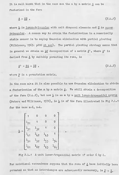
Chapter 2 The numerical solu tion o f lin e a r algeb raic equations 19

2.1 The solution, o f trian gu lar systems 21

2.2 The lin e a r least-squares problem 24

2.3 Cholesky decomposition o f the normal equations 27

2.4 Gaussian elim ination 23

2.5 The use o f orthogonal transformations 34

2.6 The m odified Gram-Schmidt method 3&

2.7 The method o f Householder transformations ■ 40

2.8 C la ssica l plane ro ta tio n s 43

2.9 Modern plane ro ta tio n s 40

2.10 A comparison o f the p la n e-rotation methods with

other methods based upon orthogonal transformations

61

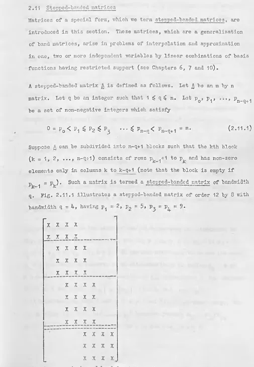
2 .1 1

Stepped-banded matrices

69

2 .12

T ria n gu la r!

2

ation o f stepped-banded matrices using

Gaussian elim ination

70

2.13 Triangu.larizatioii o f stepped-banded matrices using

v i i

2.14 Orthogonal t r*i angular i z at :i. on o f stepped-bandcd

matrices using plane ro ta tio n s 79

2.15 The singular value decomposition 82

2.16 Perturbation bounds f o r the solu tion o f lin e a r

systems

87

Chapter 3 B--splines and th e ir numerical evaluation $2

3.1 D e fin itio n o f a spline function 93

3.2 The d e fin itio n o f a B-spline 93

3.3 The conventional method o f evaluating B -splines 101

3.4 A recurrence re la tio n fo r B-splines 103

3.5 The values o f B-splinos at the ends o f the range 111

3.6

The sum o f normalised B-splines and bounds fo r

th e ir values

112

3*7 A p o s te rio ri error bounds fo r the values o f

'B-splines computed from divid ed d ifferen ces 115

3.8

A p o s te rio ri error bounds fo r the values of

B-splines computed by the method o f convex

c ombinat ions 117

3.9 A p r io r i error bounds fo r the values o f B-splines

computed by the method o f convex combinations ’ 119

3.10 The e ffe c t s o f perturbations in the data 122

3 .11

Numerical examples

123

3.12 The evaluation, fo r a prescribed argument, o f a l l

non-zero B-splines o f order n 129

3.13 Other methods fo r evaluating B -splines 134

Chapter 4 D iffe r e n tia tio n and in tegra tio n o f B-splines 137

4 .1

Recurrence r e la tio n s fo r the d e riva tives o f

140

145

149

150

157

156

162

164

170

172

175

181

18

?

195

203

205

208

209 The d eriva tives o f the E -splines at the ends o f

the range

The d eriva tives o f B-splines at the knots

Algorithms fo r the evaluation o f B-spline

d eriva tives

The d e fin ite and in d e fin ite in te g ra ls o f

B-splines

The B-spline representation o f splines and

polynomials

The B-spline representation o f splines

The numerical evaluation o f a spline from i t s

B-spline representation

Error analyses o f algorithms fo r evaluating a

spline from i t s B-spline representation

The e ffe c t o f errors in the B-spline c o e ffic ie n ts

on the computed value o f the spline

The B-spline representation o f powers

Algorithms fo r computing the B -spline c o e ffic ie n ts

The B-spllne representation o f polynomials

Error analyses o f the algorithms fo r computing

B -spline c o e ffic ie n t s

The d eriva tives o f a spline represented dn

E-spline form

The in d e fin ite in te g ra l o f a spline represented in

B -spline fo r a

Representation in piecewise - Chebyshev-series

form

Spline in te rp o la tio n

i x

6

»2 The lin ea l' system: form ation - 210

6-3 The lin e a r system: solu tion 213

6.4 Algorithms f o r the spline in te rp o la tio n problem 213

6.5 Error analysis 217

6.6

M u ltiple knots

223

6.7

The choice o f e x te rio r knots

223

6.8

A conjecture re la tin g to the'ch oice o f in te r io r

knots and comments on the "well-posedness" o f the

spline in te rp o la tio n problem 226

6.9 Numerical examples 233

Chapter 7 Least-squares spline approximation 242

7 „1 The least-squares s p lin e - fit t in g problem 243

7.2 Method o f solu tion 244

7.3 An algorithm f o r least-squares spline

" approximation

248

7c4 Error analysis 250

7 .5

S e n s itiv ity o f the B-spline c o e ffic ie n t s to

perturbations in the data 256

7.6 The important case o f cubic splines 259

7.7 Assessing the a c c e p ta b ility o f a least-squares

cubic-spline approximation

262

7*8

The choice o f knots 264

7*9 Numerical examples • 266

7.10 Automatic knot s e le c tio n 284

7

« T1 Least-squares spline approximation o f a

mathematical function

287

Chapter

8

Spline f i t t i n g with convexity and concavity

constraints ■

291

8 .2

8.3

8.4

8.5

Chapter 9

9.1

9.2

9.3

9.4

9.5

Chapter 10

10.1

10. 2

10.3

10.4

10.5

10.6

References

A class o f constrained lin e a r approximation

problems

293

A representation o f cubic splines 2'j6

Constrained cu bic-spline approximation 301

Numerical examples • 305

The imposition o f boundary conditions and other

e q u a lity constraints

315

The im position o f a sin gle d e r iv a tiv e boundary

condition 315

Im position o f a set o f boundary conditions 318

Simple point constraints

320

Compound point constraints 320

Stable methods f o r the im position o f general

lin e a r constraints

321

M u ltiva ria te splines 327

In terp ola tion c f data on a rectangular mesh by

a tensor product o f u nivariate functions

327

Least-squares approximation to data on a

rectangular mesh by a tensor product of

u n ivariate functions 330

In terp ola tion and least-squares approximation to

data on a rectangular mesh by b iv a r ia te splines

₃₃₂

The general least-squares m u ltiva ria te spline

approximation problem 335

The im position o f constraints 339

Evaluation o f a m u ltiva ria te splin e from i t s

B-spline representation 341

INTRODUCTION

ITany computations with polynomials have been, systematised in the la s t

two decades by the use o f Chebyshev s e rie s . Expressing the approximate

solution to a wide v a r ie ty o f problems as a polynomial in i t s Chebyshev-

series form has o ften proved extremely b e n e fic ia l. One o f the main

b en efits o f th is approach stems from the fa c t that in many applications

Chebyshev polynomials form an extremely w ell-conditioned basis f o r the

class o f polynomial functions. Examples o f the application o f Chebyshev

se rie s abound: in the f i e l d s o f fu n ction and data approximation,

in te rp o la tio n , quadrature, d iff e r e n t ia l equations and in te g ra l equations

are to be found many in te re s tin g and p ra ctica l re s u lts .

Polynomial splines are a gen era liza tio n o f polynomials in that a spline

o f order n includes, as special cases, a l l polynomials o f degree le s s

than n. We tre a t in some d e ta il in th is work what we consider to be a

splin e counterpart to the Chebyshev polynomials, v iz the B-splines. The

B -splines o f a given order defined upon a prescribed set o f knots form

f o r many purposes a w ell-conditioned basis f o r the class o f splines o f

that order with che same knots. Moreover, the B -splines too have

ap p lication to many problems in numerical analysis, including those

re fe rre d to above. Considered here are some o f the properties o f

B -splines, many o f which are new, and ways in which these properties can

be u t ilis e d to advantage in problems o f in terp o la tio n and approximation

o f d iscrete data.

The theory o f splin es has made s ig n ific a n t advances, p a rtic u la rly in

the la s t decade (see the bibliography by van R ooij and Schurer, 1973)»

a ft e r a r e la t iv e ly quiet period fo llo w in g the pioneering work o f

algorithms f o r spline compuiaxions has lagged s ig n ific a n tly behind the

th e o re tic a l development. Accordingly, in order to swing the balance a

fr a c tio n in favour o f the p ra c tic a l sid e , our approach i s predominantly

algorithm ic. We concentrate upon the development o f what we b e lie v e are

fundamental and useful algorithms f o r computing with splines expressed

in th e ir B-spline form* Many o f these algorithms are supported by

p ra c tic a l re su lts as w ell as by rigorous erro r analyses, the l a t t e r

often in d ica tin g the degree o f s t a b ilit y o f the algorithms.

Of the ten chapters in th is work the f i r s t f i v e con stitu te "backbone"

chapters upon which the remaining f i v e depend.

Chapter 1 i s prim arily expositors’- and discusses flo a tin g -p o in t arithmetic

and basic concepts r e la tin g to the erro r analysis o f computational

processes. Our approach i s e s s e n tia lly that propounded by Wilkinson

(s e e , in p a rticu la r, Wilkinson, 1955; P eters and W ilkinson, i 97l )- We

also describe the step-by-step manner in which our algorithms are

presented and what we understand by the numerical s t a b ilit y o f a

computational process.

The f i r s t part o f Chapter 2 i s also mainly expository in that methods

f o r the numerical solu tion o f lin e a r algebraic systems in both the

determined and over-determined cases are surveyed. The work o f

Wilkinson (p a r tic u la r ly Wilkinson, 1965; P eters and Wilkinson, 1970)

has again stron gly influenced our treatment. We then discuss the use

o f both c la s s ic a l and mod -m forms o f plane ( Givens) ro ta tio n s

(Gentleman, 1973; Hammarling, 1974) fo r so lvin g over—determined (le a s t -

squares) systems and g iv e reasons why we b e lie v e that plane rotation s

have advantages over other methods such as Householder transformations

x.i:ii

based on the timing analysis o f Wichmanu (

1973

) , c f the r e la t iv e

e ffic ie n c ie s o f methods f o r least-squares problems. The second part o f

Chapter 2 contains d eta iled description s o f some new algorithms f o r the

solu tion o f the structured (stepped-bended) lin e a r systems that arise

in spline in terp o la tio n and approximation problems. For the fu lly -

determined square case (in te r p o la tio n ) via give algorithms based upon

G-aussian elim in ation (GS) and elementary transformations, and for.’ the

rectangular case algorithms based upon c la s s ic a l and modern forms o f

plane ro ta tio n (P il). The G-S algorithm can be considered as a

gen eralization o f the algorithm o f Martin and Wilkinson (1367) f o r Larded

systems, and the HI algorithm as a s p e cia lisa tio n o f the Givens algorithm

o f Gentleman (1973)» Our algorithms prove to have advantages in terms

o f s im p lic ity , speed and storage over those based on Householder

transformations f o r stepped-banaed lin e a r systems given by held (

1967

)

and Lawson and Hanson (1974). F in a lly , i t i s shown that the powerful

singular value decomposition may be adapted to analyse stepped-banded

systems e f f ic i e n t l y .

In Chapter 3 polynomial splines and t h e ir properties are discussed and a

p a rticu la r form o f fundamental sp lin e, the B~spline, is introduced. A

new id e n tity (Cox, 1972) r e la t in g B -splines o f consecutive degrees is

then established. This id e n t it y , which expresses the value o f a B-spline

o f order n as a convex combination o f two B -splines o f order n -

1

, find which proves fundamental to our work, was discovered simultaneously in

the United States by de Boor (1972). We g iv e algorithms based upon the

conventional method employing divided d ifferen ces ana upon convex

combinations f o r evaluating B -splines. D etailed erro r analyses and

te s t computations are used to demonstrate con clu sively that algorithms

based upon the use o f convex combinations ore unconditionally sta b le f o r

a rb itra ry (even m u ltip le) knots, whereas algorithms employing divid ed

X-J.V

In Chapter 4 a recurrance re la tio n due to de Boor (1972) l'or the

d e riv a tiv e s o f B-splines is established. A new r e la tio n o f th is type

i s then obtained that proves to be an extension o f the fundamental

id e n t it y discovered in Chapter

3

. Two re su lts that prove to be o f

considerable use in subsequent chapters are then established: the values

o f a l l E-spline d e riv a tiv e s at the ends o f the range, as w ell as certa in

d e riv a tiv e s at the knots, can a l l be computed in an unconditionally stable

manner. A class o f algorithms due to B u tte rfie ld (1975) f o r E-spline

d e riv a tiv e s in the general case is then outlined. F in a lly , some re su lts

r e la tin g to the d e fin it e and in d e fin ite in tegra tion o f B-splines are

given : these resu lts a l l appetir apparently f o r the f i r s t time, with the

exception o f one due to B u tte rfie ld (1975)> which i s a fu rth er

gen era liza tio n o f the id e n tity o f Chapter j>, and one discovered

independently by Gaffney (

1

974).

Chapter .5 is concerned with various computations a ris in g from the

representation o f splines and polynomials in terms o f B-splines. Pc

present a p a rtic u la rly useful re su lt due to de Boor (1972) which expresses

a lin e a r combination o f B-splines in terms o f B -splines o f lower order

with certa in polynomial c o e ffic ie n t s . This re s u lt i s then -used to

establion a new proof t-ha«, the B -splines form a lin e a r ly independent set

o f basrs funccions in terms of which an a rb itra ry spline s (x ) can be

expressed, and oo esoablxsli lo c a l low er and upper bounds f o r s (x ) dn

terms o f i t s B -spline c o e ffic ie n t s . Two schemes proposed by de Boor (1972)

f o r the evaluation o f s (x ) are described and, f o r the f i r s t time, e r ro r

analyses o f these schemes, which demonstrate t h e ir unconditional

s t a b i l i t y , already observed em p irica lly by de Boor, are given. The

problem o f representing powers o f x in terns o f B -splines i s then

e r r o r analyses c a rrie d out. Methods f o r rep resen tin g in t h e ir B -splin e

form the d eriva tives and in te g ra ls o f r ( x ) are then considered.

Chapter 6 i s the f i r s t o f three "a p p lica tio n s” chapters and discusses

the in te rp o la tio n o f a data set 'ey splines o f a rb itra ry order with

a rb itra ry knot- p o sition s. A new algorithm, together with a d e ta ile d

erro r a n a lysis, i s presented f o r th is problem. Schumakor (1

96

?) has spoken o f the need f o r such an algorithm. In p a rtic u la r, i t i s shown

that i f B-splines are evaluated as recommended and i f one o f the algorithms

proposed f o r solvin g stepped-bandod systems is employed, the computed

spline i s the exact in terp o la n t o f a neighbouring data s e t. Choices f o r

tlie e x te r io r knots ( required in order to d efin e a f u l l s e t o f P-splino

basis fu n ction s) and the in t e r io r knots are discussed; in p a rticu la r the

dependence o f a certain condition number upon the p osition s o f these Imots

.is in vestig a ted using the singu lar value decomposition (SVD). Some

inform ative numerical te s ts are carried out and a p r a c tic a l problem :ia

solved.

Chapter ] i s the counterpart o f Chapter 6 in tho case where a le a s t-

squares approximation rather than an in te rp o la tin g function i s required.

A new algorithm i o r te s tin g whether a unique splin e approximant e x is ts in

any given case i s presented. F or the least-squ ares s p lin e - fit t in g

problem i t s e l f an algorithm f o r splines o f a rb itra ry order with a rb itra ry

knot p osition s is proposed. This algorithm again u t iliz e s the convex-

combinations scheme and the methods fo r stepped-banded systems and is a

gen era lisa tion o f that given by Cox and Hayes (1973) f o r cubic splin es.

An e rro r analysis o f th is algorithm is given and, with the aid o f the SVD,

an extremely encouraging conclusion i s made r e la tin g to i t s s t a b ilit y .

The important case o f cubic splin es i s discussed ar.d the question o f knot

xv.\

f i t s to re a l data sets are presented.

Chapter

8

concentrates on the typo o f problem where more information than

that contained s o le ly w ith in the data set i t s e l f is prescribed. I t i s

shown that some important types o f continuous constraints upon the

approximating spline may be enforced by imposing upon the splin e a f i n i t e

number o f point constraints. A new representation o f cubic splin es is

then used, in conjunction with sn extension to algorithms due to

Barrodale and Young (1966) f o r L.j- and L w -approximation, f o r spline

f i t t i n g subject to convexity and concavity constraints. P r a c tic a l

examples are given to demonstrate the usefulness o f tho approach.

In Chapter 9 the incorporation o f lin e a r eq u a lity constraints in spline

approximation problems i s discussed. In p a rticu la r, i t i s shown that

boundary conditions may be incorporated re a d ily by a simple m odification

to tho b a sis. For more general constraints, algorithms f o r lin e a r le a s t -

squares problems with lin e a r eq u a lity constraints are discussed.

F in a lly , Chapter 10 discusses b r ie fly the extension o f some o f the methods

o f the e a r lie r chapters to more than one independent v a ria b le . The

in te rp o la tio n and least-squares approximation to data given at a l l

v o rtic e s o f a rectangular mesh by a tensor product o f u nivariate functions

is f i r s t discussed. The case wlie.ro the u n ivariate functions tire B-splines

is then trea ted . The general problem o f the least-squares spline

approximation o f a rb itra ry m u ltiva ria te data, f o r which an algorithm has

been given in the cubic case by Hayes and H a llid a y (1974), is then

CHATTER 1

FLOATING-POINT ARITHMETIC ANN ERROR ANALYSIS

This chapter is one o f three "backbone

'1

chapters to th is work; i t serves as an introduction to flo a tin g -p o in t a rith m etic, error analysis, algorithm

and numerical s t a b ilit y . In Section i.1 vie summarise the rudiments o f

flo a tin g -p o in t arithm etic, adhering c lo s e ly to the concepts developed by

Wilkinson. In p a rticu la r, wo d e ta il those aspects o f flo a tin g -p o in t

arithm etic o f which we sh a ll make considerable usein subsequent chapters,

where we analyze a number o f computational processes relevant to spline

approximation. In Section i .2 we illu s t r a t e the type o f error analysis

vie sh a ll be carrying out by os:».mining some simple formulae fo r lin e a r

transformations and, from the re su lts o f our analyses, make a conjecture

r e la t in g to the analysis o f more general processes. We also discus.:

running error analysis and the derivation o f a p o s te rio ri and a p r io r i

error bounds. In Section 1.3 vie g iv e a b r i e f discussion o f algorithms

and what we understand by numerica l s t a b i l i t y . We also outline the way

in which we sh a ll present algorithm ic descriptions o f our computational

processes.

1.1 F lo a tin g-point arithmstj,c

Many o f the numerical methods described in the fo llo w in g chapters w i l l

be analyzed in terms o f th e ir implementation in standard binary flo a t in g ­

point a rith m etic.' In th is respect we shall fo llo w c lo s e ly the approach

o f Wilkinson (19^3, 19^5) •

A number x is termed a standard binary flo a t in,’- - poin t number i f i t car.

be represented by an ordered p air (a ,b ) such that x = a2*\ Here b, the

exponent, i s an in te g e r, p o s itiv e or n ega tive, usually r e s tr ic te d to the

Gy G

?

a, the mantissa, is a binary number, usu ally s a tis fy in g g ^ |a| < !,

with no more than t binary d ig it s . Typical values o f t l i e in the range

1

6 to 48. The value o f 2 “ is termed the r e l a t i ve machine p re c is io n .

The number aero is represented in the non-standard form a = b = 0.

A re la tio n o f the form

y = f l ( x

1

* x

2

* x^ * . . . « xn) , (1. 1.1)

where ca,ch * denotes any one o f the arithmetic operations +, - , X or

4

, im plies that , x0, . . . , x and y aro stai', darà binary flo a tin g -p o in t

numbers (o r z e r o ), and that y i s the re su lt o f performing the appropriate

flo a tin g -p o in t operations. The m u ltip lica tion sign w i l l frequ en tly be

omitted; thus x

^ 2

im plies / x ? . The d ivis io n sign (-)) w i l l frequ en tly

be replaced by slash (/ ) or a h orizon ta l lin e , in the usual way.

Parentheses on the right-hand side o f (1 .1 .1 ) are often necessary to

remove ambiguity or to emphasise the order o f the computation. Otherwise

the sequence o f flo a tin g -p o in t operations i s assumed to take place from

l e f t to r ig h t, with the usual ru les o f precedence o f X and ~ over + and

Thus, fo r example, y = fl(x .j X

7

y'* ) im plies ( i ) y^ = fl(x ^ X x ^ ),

( i i ) y - flC.vg. t y = f l ( - ^ - —— l i t ) im plies ( i ) y^ = f l f r ^ ) ,

5 6

( i i ) y

2

= n ^ '3x^ > ^i i i ) ^ ( i v ) y

4

= f i ( x

5

-x é) ,

( v ) y = f l ( y y yif) • hi/idently, any ra tio n a l arithm etic expression can be

represented in iio a tin g -p o in t arithm etic terms by compounding basic

operations o f the form y = f l ( x « x ^ )•

We assume that the rounding errors in the operations are such that

flC * ,* " ^ ) = ( -

1

’!!x

2

) ( l + e ) ,

₍

1

.

1

.

2

)

For m u ltip lica tio n and d ivis io n the value o f s w i l l bo taken as zero

i f e ith e r x or is an in te g ra l power o f 2. Y/o assume fu rth er that

re la tio n s o f the type

fi(xi±:;2) = ( x ^ g V C l + e ) ,

(1.1.4)

where s s a t is fie s (1 .1 .

3

) , also hold. Relations ( l . 1 J h) are due to Kahan (see Peters and Wilkinson, 1971) and are sometimes more convenient

than (1 .1 .2 ). In any p a rticu la r situ ation we sh a ll use e ith e r (1 .1 .2 )

or (1.1 J\) as appropriate.

Wilkinson (19^3) states that some computers have less accurate rounding

procedures than those which give the above re s u lts , but we assume (as do

Peters and Wilkinson (197"1) in a d iffe re n t context) that the d ifferen ces

are not o f great consequence.

We sh a ll also make use o f the rela tio n s

(

1+2

* ) ° <(

1

+

1

.

06

s

2

^ , _{(1 .1 .3 )}

( l -

2

- t ) “ S <

1

+ .

1

.

1282

“ *, (

1

.

1

.

6

)

where s is a p o s itiv e number (o fte n in tegral

(

1

.

1

.

6

) hold as long as s and t s a tis fy the

l ) . Relations (1 .1 .5 ) and

mild r e s t r ic t io n

s

2

_ t <

0

.

1

. _{(1 .1 .7 )}

Y/e assume throughout th is work that the in eq u a lity (

1

.

1

.

7

) i s s a t is fie d

fo r a l l (reasonable) values o f

5

that a ris e . (On the English E le c tr ic

XDF9 computer, fo r which t=39, th is means that s can be as la rge as

(

0

.

1

)

2

"^ = 5*5 X 1 0 )• R elation (1 .1 .5 ) is given by Wilkinson (

1963

:

sh a ll sometimes use re la tio n (1 .1 ,5 ) in the form

(1+2” t ) s < 1 + s2 ‘1,

where

2 t l = ( 1 .0 6 ) 2 " *

(

1

.

1

.

8

)

( 1 .1 . 9 ;

We observe that re la tio n (1 .1 .7 ) is th erefore equivalent to the in eq u a lity

52

< 0.106 .

Moreover, (1 .1 ,5 ), (1 .1 .6 ) and (1.1 .7) y ie ld

(

1+2

t)s <

1.106

(

1

.

1

.

10

)

and

(

1 -2

“) S <

1 .1 1 2

.

(

1

.

1

.

11

)

(

1

.

1

.

12

)

Throughout th is work, unless otherwise stated, a (w ith or without

subscripts or superscripts) denotes a number s a tis fy in g

]e| ^

2

- t

( 1 .1 .1 3 )

and e (again with or without subscripts cr superscripts) a number

s a tis fy in g

|e) < f A J J i *\

V •

1

• ‘W

T/e sh a ll o ften estimate the arith m etical work r

computational processes by counting the number

A long operation is one flo a tin g -p o in t m u itip li

d iv is io n .

1.2 F loatin g-poin t error analysis

equired by various

o f long operations required.

cation or one flo a tin g -p o in t

As an illu s t r a t io n o f the type o f flo a tin g -p o in t erro r analysis we s h a ll

be carrying out in subsequent chapters, we examine various formulae fo r

and

6

, where i t is important that they are ca rried cut in a m inericaU y stable manner. We w i l l see that the erro r analyses in dicate very ole-'irly

whether a p a rticu la r way o f computing the transformation is stable or

p o te n tia lly unstable and, in the l a t t e r case, the reasons fo r the in s t a ll l a t ;

Consider the lin e a r transformation

X = (2x - a - b )/ (b - a ) , (₁.₂.₁)

which maps the in te rv a l £ a ,b ] in to {^-

1

, +

1

J . When implemented in

flo a tin g -p o in t arithm etic the computed value X o f X w i l l bo contaminated

by rounding e rro rs. Our aim i s to produce a bound fo r j b x j , where

SX = X - X,

(

1

.

2

.

2

)

which holds fo r a l l x

6

M . We seek a function K (a ,b ) such that

|

6

X| ^ K (a ,b )

2

_ t . (1 .2 .3 )

I t may seem somewhat surprising that v.e employ th is formal approach to

such an apparently innocuous computation as (1 .2 .1 ). The point we wish

to stress, which we hope i s brought out ry our analyses, is that atten tion

to d e t a il is o f v i t a l importance in th is and in many other computational

processes. For instance, the nature o f the erro r introduced in forming X

i s dependent upon the precisa ordering of the basic arithm etic operations

in (

1

.

2

.

1

) and, moreover, is influenced even mora i f (

1

.

2

.

1

) i s re-expiessed

in certain other mathematically equivalent but computationally d is tin c t

forms.

Three possible ways o f carrying out the transformation are given by

(1 .2 .4 )

X _{t - a}

₅

X = 2x-(a*b)_{b-a (1 .2 .5 )}

6

X = cx - d, ( 1 . 2 .o)

where

c = 2/ (b -a ) ,

d = (a+ h )/ (b-a).

A flo a tin g -p o in t error analysis o f (1 .2 .

4

) y ie ld s

X = { ( 2 x - a ) ( l + e 1) - h } (l+ e 2) ( l + e

^)(1

iK^)/(t>-a).

(1 .2 .7 )

(1.2.8)

(1 .2 .9 )

where

iSil *

^

2

_ t ( i = i ,2 ,3 ,4 ), (

1

.

2

.

10

)

from which

SX = X-X = ( e (2x-a)+3e (2 x -a - b )}/ (b - a ),

^ 1 t—

(1.2.11)

where

lell

, , e0] <C

2

, " t l

(

1

.

2

.

12

)

Thus

£,X = e. {b / (b - a )+ x } +

3

e2X (1.2 .13)

and hence

1

cX| < { j b i / ( b - a ) + t } f t 1 . (

1

.

2

.

1

L;

y/e see immediately from (1 ,2 .1 4 ) that the error in the computed value o f

X may be appreciable i f the length b-a o f the o rig in a l in te rv a l is small

compared with the'magnitude o f b.

Analysis o f (1 .2 .5 ) and (1 .2 .6 ) re s u lt in bounds fo r £X sim ilar in form

to (1 .2 .1 4 ). This state o f a ffa ir s is p a rtic u la rly unfortunate in the

case o f the tn ir d form o f the transformation equation because the use c f

(

1

.

2

.

6

) appears to be eminently sensible i f the transformation i s to be

used fo r a large number o f x-values, since the constants c and d can be

7

A fou rth fern o f the transformation, which we now study, is u n cord;tion aily

sta b le. Consider the use o f the expression

X = { ( x - a ) - ( b - x ) } / (b -a ) _{(1.2 .15)}

to compute the value o f X . An error analysis o f th is "somewhat \;nnatural"

form gives

{ M i l + e ^ - M C l + e ^ } (l+ e

5

) ( l + e

4

) ( l + e 5) ^

>2

^ b - a

where

j u . j ^

2

“ t ( i =

1

,

2

,

3

,

4

,

5

) ,

from which

SX =

( n_ ^ f v — \ -r - ( - i.N

b - a

(1.2 .17)

(

1

.

2

.

18

)

where

h i» h l> h ! <2' t1-

(1-2-19)

Thus, since ? a ^ b, i t fo llo w s from (■'.2.18) and ( l . 2 . i y ) that

fo x j < (4 )2 " t1 .

(

1

.

2

.

20

)

Note that the form (1 .2 .1 5 ) is computational!;.- no mere expensive than

(1 .2 .A) or (1 .2 .5 ), but unlike them y ie ld s at worst a very small erro r.

We now consider b r i e f l y a second stable form, having an error round only

s lig h t ly in fe r io r to (1 .2 .2 C ). The approach is based upon carrying out

the lin e a r transformation ( I .

2

.

1

) in two stages, v iz . transformation to

the in te r v a l £ o , l j , follow ed by transformation to C~

1

, l } . Error analyses o f the "obvious" transformations

r = f-_{0“ ci. (* .}

₂

_.

_{2 1}

₎

8

X = 2X’ -1,

vrhioh carry out inns two—stage pi’ ocess, y ie ld

* ' = | r f

(1-2.22)

(

1

.

2

.

23

)

and

X = (2 X '- a )(l+ e ^ ) = (l+ c

1

) ( l + e

9

) ( l +e ^ ) * i | ( i +e^ ) , (1 .2 .2 4 )

where X' is the value o f the intermediate v a ria b le , computed values are

denoted by "bars" as usual, and.

| s . | ^

2

' t ( i =

1

,

2

,

3

,

4

)

From (1 .2 .2 4 ),

6c ( x - a ) r

5X = X-X = --- + e„<

(1.2.25)

where

b-a

hi- k l < A

4

^ -

4

-from which

M < ( 7 ) s " t l .

(

1

.

2

.

26

)

(1.2 .27)

(1.2 .26)

The transformations (1 .2 .2 1 ) and (1 .2 .2 2 ) can o f course be combined to

form the sin gle transformation

2 (t-&)

b-c (

1

.

2

.

25

)

or, expressed s lig h t ly d iffe r e n t ly , as

b-a (

1

.

2

,

30

)

I t i s r e a d ily established that the use o f (1 .2 .2 9 ) also gives an erro r

s a tis fy in g (1 .2 .2 3 ) and that the bound fo r (

1

.

2

.

30

) s a t is fie s

¡

6

X | < (

6

)

2

" t l .

9

A much more d eta iled an alysis, which takes in to account the precis's

nature o f the b it patterns in the mantissae o f the flo a tin g -p o in t

representations o f a, b and x, revea ls that fo r nearly a ll values o f those

numbers the bound (1 .2 .1k) is unduly p essim istic. In p a rtic u la r, the

analysis shows that in these cases the value o f e in (

1

.

2

.

9

) is zero,

with the consequence that in ( i .

2

.

1 1

) is zero and hence

16x| < (3)2~t i .

(1.2.32)

However, the d eta iled analysis also shows that there are values o f the

numbers a, b and x which r e s u lt in e ^ being ex a ctly equal in modulus to

2 . In these cases the bound (1 .2 .1 4 ) proves to be r e a l i s t i c and predicts

accurately the magnitude o f the actual error in the computed value o f X.

D eta iled analyses o f (

1

.

2

.

3

) and (

1

.

2

.

6

) re vea l that the corresponding

bounds are in fa c t r e a l i s t i c fo r most, rather than a few, values o f a, L

and x . I am indebted to Dr J H Wilkinson who suggested the method o f

approach to these detailed analyses.

The main conclusion to be drawn from the above r e la t iv e ly simple analyses

is that fo r s t a b ilit y the transformation should be expressed in a form

that ensures that the magnitude o f each intermediate computed quantity is

rela ted as appropriate to the length o f the o rig in a l or o f the transformed

in te r v a l. Tie see that the unstable formulae (

1

.

2

.

4

) ’, (

1

*

2

.

3

) and (

1

.

2

.

6

) a l l produce as intermediate qu an tities numbers re la te d to the absolute

value o f the untransformed v a ria b le , a number having no re la tio n to the

length o f the o rig in a l in te r v a l. On the other hand, the intermediate

qu an tities produced by the stable formulae (

1

.

2

.

13

) , (

1

.

2

.

2 1

) and

(

1

.

2

.

22

) , (

1

.

2

.

29

) , and (

1

.

2

.

30

) are a l l re la te d to the lengths o f the o r ig in a l or transformed range.

Extrapolating th is conclusion we conjecture that numerica] processes in

general are more l i k e l y to be stable i f , wherever p o ssib le, the intermediat

10

computed qu an tities are not allowed to grow too la rg e (o r , in spine

rather special instances, too sm all). The p rin cip le c e rta in ly holds fo r

Gaussian elim in ation , fo r i t is known (fie ld , 1971) that whatever stra tegy

(whether i t he p a r tia l p iv o tin g , complete p ivo tin g , p ivo tin g down the

main diagonal, e tc ) is employed, a hound fo r the departure o f the lin e a r

system actu a lly solved from that req u ired to he solved is re la te d d ir e c t ly

to the la rg est matrix element at any stage o f the reduction. I f a lin e a r

system (square or rectangular) is solved using orthogonalization methods

then no growth can occur (P eters and Wilkinson, 1970), with the re s u lt

that the process i s sta b le.

In the numerical methods we discuss we adhere to th is general p rin cip le

wherever p ossib le. P a rticu la r instances are the use o f plan

0

rotation s

(Chapters 2 and 7 ), elementary s ta b ilis e d transformations (Chapters 2 and

6

) and the taking o f convex combinations. The la t t e r process is basic to

many o f our computations (Chapters k, 9,

6

and 7 in p a rtic u la r).

We do not reproduce error analyses o f w ell-accepted numerically stable

methods such as the modified Gr'am-Schmidt process, Householder

transformations and c la s s ic a l Givens ro ta tio n s fo r solving lin ea r systems,

since such analyses abound in the lit e r a t u r e , the key reference being

Wilkinson (1 9 » 5 )• However, wherever appropriate, we analyze methods that

have appeared recen tly or have been developed during the course o f th is

work.

Y.'e s h a ll carry out, in la t e r chapters, flo a tin g -p o in t error analyses o f

various recurrence re la tio n s which a rise in the solution o f lin e a r systems

and in certa in computations with splin es. In p a rticu la r we s h a ll sometimes

( i ) employ a "running" erro r analysis (P eters and Wilkinson, 1971) to

enable the computer i t s e l f to determine rigorous bounds on the errors i t

11

occasion ally, ( i i i ) obtain a p r io r i absolute or r e la t iv e error bounds.

To giv e the fla vo u r o f the types o f re s u lts re obtain we analyse a simple

example.

Consider the fo llow in g recurrence re la tio n which defines and generates

the Fibonacci numbers:

f = f . •h

fr “ f r - i + f r

-2

( r -

2

» 3 » « - * ) ^

(1.2.33)

Suppose th is computation is carried out in flo a tin g -p o in t arith m etic.

Let f denote the computed value o f f^ and b?r = f r ~ fr • Then

1 =

r , =

f , 6 f = o

o 0

f , , f-f. = _{1 1}

0

and

Thus fo r r ^ 2,

(1.2 .34)

f r = f l ( f r _ 1+ fr _ 2) = ( f r _ i+ fr _2) / ( l + e r ) ( r = 2 , 3 , . . . ) . (1.2.35)

(

1

+e ) f = f + f

0

' r r r

- 1

r

-2

(1.2.36)

and th erefore

f +_r

6

f +_{r r r} b f = f _r

_-1

+

6

f _ ,+ f _r

_-1

_r

_-2

_+

6

f _r

_-2

0

The use o f (1 .2 .3 3 ) reduces (

1

.

2

.

37

) to

(1 .2 .3 7 )

6

f = £ f , + t f c-e f ._{r r-1 r}

_-2

_{r r (1.2 .38)}

Thus

t f r | S

_(1.2.39)

12

Fo = F, -

0

..

P = S>

r r-

-1

r+P

-2

+ f r

J

(

1

.

_(■1.2.AO)

So, at the same time as i t forms the f^ , the computer can form the values

F . Such a process is c a lle d a running erro r analysis. However, lik e the

f . the values o f F cannot ha formed ex a ctly , since rounding errors are

r r

made in computing the erro r r e la tio n (1 .2 .4 0 ): This apparent d i f f ic u lt y

is e a s ily overcome as fo llo w s . Let F be the computed value o f F^. Then

the computational equivalent o f (

1

.

2

.

40

) 3s

F = f l ( F ,+P 0+ f )

r r

- 1

r

-2

r

= f ( F ,+F 0) ( U e, ) + f ! ( l +

2

„ )

1

/ r

-1

r -

2

/v

1

, r ' r j v

2

,r (

1

.2.41)

Thus, since the F^ and tho f^ are non-negative, the contribution tc the

erro r incurred in computing from (1 .2 .4 0 ) is at most a m u ltip lic a tiv e

-t -2

fa c to r (1-2 ) . Hence, since 6 fo= 6 f)=0,

j f f r | .<

2

“ t ( i -

2"t )2

2

rF.

Notì, by v irtu e o f (

1

.

1

.

12

) ,

( l -

2

_ t ) 2_2r <

1

.

1 1 2

.

Hence, since F >

0

fo r r ^

2

,

(1.2.42)

(1.2.43)

|of.| < (

1

.

112

)

2

" * Fr . ( r >

2

) . (

1

.

2

. V i)

This I’ esu lt i s an a p o sterio ri absolute error bound. Although such a

re s u lt is extremely useful in. p ra c tic e in that it. enables a rigorous

bound on the absolute error in the computed value to be obtained, i t t e l l s

us nothing about the q u a lita tiv e nature o f the e r r o r growth in the

computation. In other words i t does not t o l l us whether the bound grows,

13

certain -favourable case» the running er.ror analysis approach can give

r is e to a p o s te rio ri bounds which not only display th e ' q u a lita tiv e nature

o f the growth but also obviate the need a ctu a lly to use a running error

rela tio n sh ip lik e (

1

.

2

-

40

) (which, imvi d en ta lly, requires even more

computational e ff o r t than the basic recu rren ce!). For instance, fo r the

above example we sh a ll show th at, fo r r

2

, F^ s a t is fie s the in eq u a lity

Fr ^ (l4 2 " t ) r " 2( r - l ) f r , (1-2.45)

and hence that

¡5 f r j ^ 0 +2~t ) r " 2(r - l ) 2 * 't f r . (1 .2 .46)

In order to establish th is re s u lt we f i r s t assume i t to be true fo r

24

,, F , ^ Then the substitution o f (1.2 .45) (w ith r - i and then

r

-2

replacing r ) in to the right-hand side o f (

1

.

2

.

40

) and the use o f (

1

.

2

.

36

) gives

Fr < (l+ 2 " t ) r " 3( r - 2 ) f r _ 1- .(l+2-t ) r ^ ( r - 3 ) f r _ 2H-fr

< ( l +2-t ) r " 3 { ( r - 2 ) ( f r _ 1+f ^ 2)+'fp )

^ (

1

+

2"t )r " 3

[ ( r -

2

) ( l +

2

‘ ! ) f r+ f r ]

< ( i + 2 " t ) r “ 2( r - l ) f r . (1.2 .47)

But from (1 .2 .4 0 ), F

2

= f^ . Ileneo (1.2 .45) is true fo r r - 2 and by induction th erefore fo r a l l r

2

.

Having established a re s u lt o f the form (1 .2 .4 5 ), i t may then be possible

to obtain an a p r io ri r e la t iv e error bound. F ir s t ly (1 .1 .1 1 ) is used to

' \

sim p lify (1.2 .45) s lig h t ly to give

Vr $

1

.

106

( r - l ) f r (1 .2 .4 8 )

14

K r-1 )

But the r e la t iv e error in f is simply

f - f

r r i fr M / ?r

f_X* f r - b fr

1

- i f r / f r

t

\4.? iiS -)

f

\ «¿1r\ ₀₎

/ 1.1Q6(r-i)2~'t

1-1.106(r-l)2“ t

<

1

•I

06

( r - l )

2

" t

1-0.1106

< 1.244(r~l)2_ t , (1.2.51)

using (

1

.

1

.

7

)* V/e can th erefo re sta te, befo re the computation is sta rted ,

that the r e la t iv e error in the computed value o f f cannot exceed

1

,? 4 4 (r -l)2 l’ . This re s u lt i s absolute 3.y r i r orov.s; in practice the

s t a t is t ic a l e ffe c t s o f rounding errors are more l i k e l y to give an actual JL _j0

error o f the order o f ( r - l ) ‘ 2 . However, the importance o f a resu lt o f

the type obtained here is not only that the precise natui’e o f the error

bound has been obtained, but also that an a p r io r i erro r bound car. be

obtained at a i l and, as we w i l l see in Section i t h a t the computation

has he«ii shown to be unconditionally numerl m i? stable.

1

.5

Algorttluas and numerical s t a b ilit y

An a lg o r it hm is a procedure (s e t o f ru les , re c ip e ) fo r obtaining a solu tion

to a s p e c ific mathematical problem. An algorithm describes in an

unambiguous manner the way in which a requ ired o<4c c f numbers, the

solut io n , may be computed from a given set o f numbers, the data. For

instance, the recurrence r e la tio n (

1

.

2

.

35

) constitu tes an algorithm fo r

computing the Fibonacci numbers f _ , f „ , . . . from the data ( i n i t i a l conditions)

15

Let the m-vector x denote a set o f data values supplied to an algorithm L,

Let the n -vcctor f denote the solution obtained by A u-sing exact

arithm etic and the n~vector f the solu tion obtained by A using standard

flo a tin g -p o in t a rith m etic.

Every algorithm has a domain o f applicab i l i t y X (R ice, 1971; Cox, 1974),

defined by the set o f data x fo r which the algorithm can provide the

desired solution f . For instance, X = j x«£- 0j fo r an algorithm which

computes the p o s itiv e square root o f a r e a l number x; in p ra ctice there

w i l l be an upper bound M fo r the values o f x fo r which the algorithm i s

designed, in which case X = ^x j 0 $ x ^ Li j .

A w i l l be termed unconditional l y numerically stabile i f , fo r a l l :: G X,

the implementation o f A in standard flo a tin g -p o in t arithm etic provides a

solution f which in some sense bears a close resemblance to f . Probably_{fv* MM^**""**** 1~~IT '■ r\t}

the most desirable form o f closeness is

IlH lU v ' * Hill -

(1 .3 .1 )

where

2

is the r e la t iv e machine p recisio n , as b efore, and K,, is re la teu to the p a rticu la r process employed in A. jj . jj denotes any convenient

vecto r norm«. I f the computed solution is a sin gle value then || . jj may

be replaced by j . j in the usual way. Often, fu r a p a rticu la r process,

.is e ith e r a constant or depends upon a small number o f parameters

r e la t in g to that process. Sometimes an expression fo r K, can be determined

* 1

a p r i o r i ; in other cases K, may be the re s u lt o f a running error analysis

or an a p o s te rio ri analysis.

I f K^2 1 then (1.3• 1) may be considered an ex cellen t bound in that the

r e la t iv e error in the computed solution w i l l be small.

Sometimes i t may oe d i f f i c u l t or impossible to obtain a bound o f the form

16

fl-i

II <

V "V

(1.3.2)

where, as b efo re, Kg i s a constant or i s r e la te d to the p a rticu la r

process, but

M = max // T I/’ .

x

6

X

v t

0 - 3 . 5 )

L. i then 0 .3.2) may also in dicate a stable algorithm. Of course,

(

1

.

3

.

2

) i s a somewhat weaker- re su lt than (

1

.

3

.

1

) in that whereas

( 1 . 3 , 1 )

gives a bound on the r e la t iv e erro r and, consequently, on the absolute

e rro r, (

1

»

3

.,

2

) merely gives a bound on the absolute erro r, which may or may not imply a s a tis fa c to ry r e la t iv e error bound.

An algorithm w i l l he termed co n d itio n a lly numerically stable f f a re s u lt

o f the form (1 .3 - 0 or 0 - 3 - 2 ) holds fo r an id e n tifia b le subset X' o f X.

For some algorithms i t is not easy to quote a re s u lt as straightforw ard as

(1-3-1 ) or (■ -

3

-^/

1

, oven i f such a re s u lt can be obtained at a l l . However, we can sometimes say that a p a rticu la r algorithm is "good" because i t

fx b ib t t s Stable behaviour in practice fo r most, x

6

X, although no th e o re tic a l

statement o f behaviour is e a s ily obtained. The values o f x G X fo r which

the algorithm f a i l s to produce good re su lts may correspond to path ological

or extreme situ a tion s, eg to data sets u n lik ely to ¿ ris e in p ra c tic a l

a p p lica tio n s.

For some algorithms rigorous erro r bounds can be determined, but the bounds

are most u n lik ely to be attained or even approached at a l l c lo s e ly . A good

example i s the bound associated with Gaussian elim ination with p a r tia l

p ivo tin g fo r solvin g lin e a r algeb raic systems (F ilk in son ,

1965

:p

97

) , which contains a fa c to r o f 2 , where n is the order o f the system. I t might

be thought th erefo re that fo r systems o f quite modest size tbs - - i.

17

However,- nothing could 'be fu rth er from the truth since, apart from

a r tific ia lly - c o n s tr u c te d examples ( f o r an in te re s tin g example see

Wilkinson, 1961), a more r e a l i s t i c , though not rigorou s, bound fo r

p ra c tic a l purposes contains a fa c to r o f the order o f unity rather then

„n-1

Most o f the above discussion re la te s to fo rward error analysis in which

a measure o f the closeness o f the computed solution to the actual solution

i s sought. Per many algorithms i t i s more meaningful and releva n t to vise

a baolrward error analysis. In such on analysis the solu tion obtained is

in terp reted as the exact solution o f a problem with data x which is

(h o p e fu lly ) only s lig h t ly d iffe r e n t from x. Bounds upon

j|

x~x

J|

are then sought, which again in dicate whether the algorithms can be considered as

being numerically stable.

Many o f the computational processes we discuss ere accompanied by

commented algorithms. These algorithms ere intended to provide a

d e fin it iv e "

1

nterfo.ee" between a "casual" description o f a computational process and i t s formal implementation in a h ig h -le v e l language such as

A lg o l or Fortran. Ve b e lie v e that a reader knowledgeable in a. h ig h -level

language would re a d ily be able to code these algorithms. For commercial

reasons we are unable to l i s t actual codes in th is work. However, a l l the

algorithms presented here have been programmed in A lg o l 60, Fortran FT or

Babel, an A lg o l- lik e language due to Scowen (

1969

) . Apart from the

r e l a t i v e ly t r i v i a l illu s t r a t iv e algorithm s, such as Algorithm 1.3.1 below,

they have been tested c a re fu lly on a wide v a rie ty o f both model and

p r a c tic a l problems.

\7e use the algorithms as b u ild in g blocks, je s t as procedures are used in

A lg o l and subroutines in Fortran . Pul example, the r e la t iv e ly simple

algorithms in Section

2 ,1

fo r solvin g tria n gu la r systems are needed by

in the subsequent sections o f Chapter

2

. In turn, the algorithms in Chapters

6

and 7 fo r spline in te rp o la tio n and least-squares spline approximation make use o f the algorithms fo r lin e a r systems.

Each algorithm i s described by a sequence o f steps or stages. Most steps

describe one or more o f the fo llo w in g operations: assign a value to a

v a ria b le ; advance or return to a stated step i f a condition is s a t is fie d ,

execute the stated steps the stated number o f times. These three types o f

step occur freq u en tly. Occasionally we need to make use o f a dummy

statement (o r n u ll op era tion ), io a statement whose presence is necessary

to describe unambiguously the flow o f a computational process. For th is

n u ll operation wo borrow the term Continue from the Fortran language.

Other types o f step also appear; we b e lie v e that most o f these are s e lf -

explanatory: q u a lific a tio n w i l l be given where thought necessary. TThere

appropriate the algorithm ic steps are in terspersed by comments or remarks

which help r e la te the various stages o f the algorithm to those o f the

computational process being implemented. In p a rtic u la r, i f a special

storage strategy is employed, such as in the algorithms o f Sections 2.12 to

2 .14

fo r stepnod-banded matrices, the algorithm ic steps r e fe r to the

notation appropriate to the sp ecia l stra teg y, whereas the comments r e fe r to

the natural storage notation.

As a very simple illu s t r a t io n o f the form o f our algorithms, the recurrence

r e la tio n (1.2.337 fo r generating the Fibonacci numbers i s described by

Algorithm 1.3*1 below.

Algorithm 1.3*1: Generation o f the Fibonacci numbers f . f ... f .

— —--- o

1

n

Comment: I n i t i a l i z a t i o n .

Step 1. Set i Q = 1 and f = 1.

Comment; ilecur the defin in g r e la tio n fo r the Fibonacci numbers.

Step 2. For r = 2 ,3 ,.. .,n form f - f , + f

19

CHAPTER 2

THE NUMERICAL SOLUTION OP LINEAR ALGEBRAIC EQUATIONS

Frequent use i s made throughout th is work o f methods fo r the solution o f

systems o f lin e a r equations (Chapters

6

,

8

arid 10) and also fo r the le a s t-

squares solu tion o f systems o f over-determined lin e a r equations (Chapters

7

and 10). Accordingly, th is chapter i s devoted to the description o f numerical

stable methods fo r solvin g such problems. We concentrate p a rtic u la rly upon

the lin e a r least-squares problem, since the solution o f a system o f lin e a r

equations can be considered as being included as a special case. The lin e a r

least-squares problems that a rise from the use o f polynomial splines as

approximating functions tend to be h igh ly structured, i f a su itable basis

fo r the spline is employed. The so -ca lled observation matrix (S ection 2.2)

proves to have special properties in that many o f i t s elements are aero and,

moreover, the d isp osition o f the non-zero elements can be characterized in

a straightforw ard manner. Sim ilar remarks apply to the systems o f lin ea r

equations a ris in g from spline in te rp o la tio n problems.

In order to obtain e f f ic i e n t algorithms fo r solvin g these problems i t is

important to take advantage o f the special structure o f these matrices.

F ir s t l y , however, we outline a number o f methods cu rrently a vailab le fo r

the solu tion o f dense lin ea r least-squares problems and consider subsequently

ways in which they can bo modified so that structured problems can be trea ted .

There are six methods in current use:

( i ) Choleskv decomposition o f the normal equations ,

( i i ) Gaussian elim ination

( i i i ) Gram-Schmidt orthogonalization

( i v ) Householder transformations

( v ) Givens rotation s

(v.i) The singular value decomposition

applied to the

2 0

For our purposes the use o f Givens ro ta tio n s proves to be most appropriate.

In order to establish th is we g ive a b r i e f description o f each approach,

together with i t s merits and demerits.

In an attempt to obtain the utmost numerical s t a b ilit y , the methods applied

to the observation matrix are sometimes implemented so as to include a

column-interchange (p iv o tin g ) strategy (see, fo r example, Golub, 1965;

Businger and Golub, 1965 and Peters and 'Wilkinson, 1970). Unfortunately,

the interchanging o f columns tends to destroy the nature o f the sero-non-

sero structure. Since in our work we wish to take f u l l advantage o f

structure, we would be prepared to accept a s lig h t loss o f numerical

s t a b ilit y i f the avoidance o f column interchanges le d to s ig n ific a n t ly more

e f f ic i e n t algorithms.

There i s evidence both em pirical and th e o r e tic a l that the behaviour o f the

m odified Gram-Schmidt method (see Section 2.6) is not improved by column

interchanges. For instance, a fte r obtaining considerable computational

evidence, Rice (

1966

) concluded that interchanges re s u lt in a perceptible

but small (even n e g lig ib le ) improvement. In a detailed! th e o re tic a l flo a tin g ­

point error analysis Bjftrck (

1967

) concluded th a t, regardless o f whether or

not interchanges are made, the errors in the computed solution are less

than the errors re s u ltin g from r e la t iv e perturbations in the observation

matrix and right-hand side o f K(m,n)2 \ Here t is the number o f b it s in

the mantissa o f the flo a tin g -p o in t word and K i s a modest function o f m and n

(th e resp ective numbers o f rows and columns in the observation m a trix ).

Sim ilar conclusion can be expected to hold in respect o f methods ( i v ) end

( v ) (V/ilkinson, 1974).

Many o f the numerical methods v/e describe are applicable equally to the

square case (in te rp o la tio n ) and to the rectangular or over-determined case

(le a s t squares). However, there are advantages to be gained in terms o f