MISSION PERFORMANCE EVALUATION FOR SOLAR SAILS USING A
REFINED SRP FORCE MODEL WITH VARIABLE OPTICAL COEFFICIENTS
Andreas Borggräfe
RWTH Aachen University, Germany
Bernd Dachwald
FH Aachen University of Applied Sciences, Germany
ABSTRACT
Solar sails provide significant advantages over other low-thrust propulsion systems because they produce thrust by the momentum exchange from solar radiation pressure (SRP) and thus do not consume any propellant. The force exerted on a very thin sail foil basically depends on the light incidence angle. Several analytical SRP force models that describe the SRP force acting on the sail have been established since the 1970s. All the widely used models use constant optical force coefficients of the reflecting sail material. In 2006, MENGALI et al. proposed a refined SRP force model that takes into account the dependancy of the force coefficients on the light incident angle, the sail’s distance from the sun (and thus the sail temperature) and the surface roughness of the sail material [1]. In this paper, the refined SRP force model is compared to the previous ones in order to identify the potential impact of the new model on the predicted capabilities of solar sails in performing low-cost interplanetary space missions. All force models have been implemented within InTrance, a global low-thrust trajectory optimization software utilizing evolutionary neurocontrol [2]. Two interplanetary rendezvous missions, to Mercury and the near-Earth asteroid 1996FG3, are investigated. Two solar sail performances in terms of characteristic acceleration are examined for both scenarios, 0.2 mm/s2 and 0.5 mm/s2, termed “low” and “medium” sail performance. In case of the refined SRP model, three different values of surface roughness are chosen, h = 0 nm, 10 nm and 25 nm. The results show that the refined SRP force model yields shorter transfer times than the standard model.
INTRODUCTION
1. SOLAR SAIL FORCE MODELS AND PERFORMANCES
1.1 Standard and Refined SRP Force Model
[image:2.595.175.428.258.413.2]For the description of the solar radiation pressure (SRP) force exerted on a solar sail, it is convenient to introduce two unit vectors in a sail-fixed 2D reference frame S = {n, t}, as shown in Fig. 1 (because of symmetry, the third dimension is not relevant here). The first one is the sail normal vector n, which is perpendicular to the sail surface and always directed away from the sun. The second unit vector is the sail tangential vector t. Further, let O = {er, et, eh} be an orthogonal right-handed coordinate frame, where er points always along the sun-spacecraft line, eh is the orbit plane normal (pointing along the spacecraft’s orbital angular momentum vector), and et completes the right-handed coordinate system (er× et = eh). Then in O, the direction of the sail normal vector, which describes the sail attitude, is expressed by the pitch angle α and the clock angle δ.
Fig. 1. Definition of the sail normal vector and the thrust normal vector and sail angles [1]
At a distance r from the sun, the SRP is
2 2
0 0 0
2 μN 4.563
m
S r r
P
c r r
(1)
Where S0 = 1368 W/m2 is the solar constant, c is the speed of light in vacuum, and r0 = 1 AU. The standard SRP force model for non-perfect reflection from Wright in Ref. 4 uses the set of optical coefficients P = {ρ, s, εf, εb, Bf,
Bb} to parameterize the optical characteristics of the sail film. Here, ρ is the reflection coefficient, s is the specular reflection factor, εf and εb are the emissivity coefficients of the front and back side, respectively, and Bf and Bb the non-Lambertian coefficients of the front and back side, respectively, which describe the angular distribution of the emitted and the diffusely reflected photons. It can be shown, that the SRP force has a normal component Fn (along
n) and a tangential component Ft (along t) with
(2a)
(2b)
and the thermo-optical SRP coefficientsa1 f s( , ),
a2 f s( , ,
B Bf, , , ),b
f b a3 f s( , )
, as defined in [1]. Addition of the two force components Fn and Ft results in the total thrust vector Fm, which points along the direction of the SRP force. Its direction is described likewise by the cone angle θ and (again) the clock angle δ. The total SRP force can then be written ascos m
F PA
m , with
a1cosa2
2 a3sin
2 (4), (5)
1 2
2
cos cos
cos sin
n
t
F PA a a
F PA a
, where Ψ depends only on the pitch angle α and the optical coefficients P of the sail film.
The refined SRP force model introduces a dependancy of the optical coefficients ρ and s on the pitch angle α (or light incidence angle) and the mean surface roughness h (in nm), which quantifies the number of micro-irregularities with a certain height distribution. Moreover, the emissivity coefficient ε depends on the current sail equilibrium temperature (SET) and thus on α and the spacecraft-sun distance r. Thus, the optical properties of the sail film are no longer assumed to be constant. All dependencies of the optical coefficients can be summarized as
( ),
( , ),
(
)
( , )
f
s
f
h
f SET
f
r
(7)Conclusively, the optical SRP coefficients a1, a2 and a3 are no longer constant. The functional representation of ( ) and ( , )
f s f h
[image:3.595.59.535.310.482.2] was experimentally discovered by using unpolarized solar light on a reference sail film with a highly reflective aluminum-coated front side and a highly emissive chromium-coated back side [3]. The resulting curve fits are visible in Fig. 2. With increasing surface roughness, the fraction s of specularly reflected photons is decreasing.
Fig. 2. Reflection coefficient ρ (left) as a function of the pitch angle α and specular reflection coefficient s (right) as a function of the pitch angle α and the surface roughness h [1]
Here, h = 0 means zero surface roughness and thus all photons which are not absorbed are specularly reflected (no diffuse reflection). However, this case does not represent a perfect mirror (ideal sail), since a fraction of the incident photons is absorbed by the sail (ρ (α) < 1). For the ideal sail, ρ (α) = 1. The surface emissivity εf and εb is found to be a function of the SET and can be expressed through a best-fit second order polynomial expression having semi-experimental origin [1],
(8)
, where Tf b, is the reference temperature of the employed material and ci are experimentally obtained material-specific polynomial coefficients for Al|Cr [1]. Since the emissivity ε is no longer assumed to be constant but depending on the SET, the temperature needs to be calculated as a function of sun-sail distance and sail pitch angle. By using a sixth order polynomial expression of the sail equilibrium temperature T
d T6 6d T5 5d T4 4 d0 (9)
, with the parameter d0 defined as
2 , 0, , 1, . .
(
.)
2, ,(
.)
f bc
f bc
f bT T
f bc
f bT T
f b
(10)
The other parameters d6, d5, d4can be found in Ref. [1].When the current equilibrium temperature of the solar sail is found, the corresponding front and back side emissivity εf and εb can be calculated.
1.2Sail Model Performances and Comparison
The most commonly used solar sail performance parameter is the characteristic acceleration ac. It is defined as the SRP acceleration acting on a solar sail that is oriented perpendicular to the sail-sun line (n = er) at r0(1 AU). For the non-perfectly reflecting SRP force models (standard and refined), it is
0
1 2
(
)
c
P A
a
a
a
m
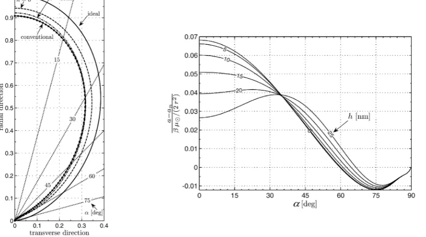
(11) [image:4.595.78.511.398.639.2], where P0 = P (r = r0), m is the sailcraft mass, and A is the sail surface area. In order to access the capabilities of the refined force model in comparison to the other models, the set of possible SRP acceleration vectors can be illustrated by a so-called “a-bubble”. Fig. 3 shows the a-bubble shapes for the ideal, standard and refined force model, projected in the orbit plane (er , et). The scales are normalized with the maximum ideal acceleration value. Each bubble represents the set of possible force vectors for each sail model and is the surface on which the tip of the a-vector is constrained to lie. The difference of the total acceleration for the refined model compared to the standard model (a – an) in dependence on α is also shown in Fig. 3.
Fig. 3. Left: Shapes of the a-vector bubbles for the ideal, standard and refined SRP force model. Right: Difference of sail accelerations ‘a’ of the refined and standard SRP force model ‘an’ [1]
Here, an is the acceleration of the standard model. The scales are again normalized to the maximum ideal acceleration. It is visible that for a pitch angle α≥ 60° the standard model marginally exceeds the performances of the refined model (≤ 1%). The refined model with a surface roughness of h = 25 nm is only slightly better than the standard model, whereas for the lowest surface roughness h = 0 nm the performance is the highest among all force
2
4 0 0
0 2 0
(1 ( )) cos
( , ) [K ] Bol
W r
d d r
r
models. Nevertheless, this is only true for α < 35°. Above this value sails with a high surface roughness slightly exceed the performance of sails with a low surface roughness.
2. TRAJECTORY OPTIMIZATION AND EVOLUTIONARY NEUROCONTROL
Within this paper, evolutionary neurocontrol (ENC) is used to calculate near-globally optimal trajectories. This method is based on a combination of artificial neural networks (ANNs) with evolutionary algorithms (EAs). ENC attacks low-thrust trajectory optimization problems from the perspective of artificial intelligence and machine learning. Here, it can only be sketched how this method is used to search for optimal solar sail trajectories. The reader who is interested in the details of the method is referred to Refs. [2] and [5]. The problem of searching an optimal solar sail trajectory x*[t] = (r*[t],r*[t]) – where the variable [t] denotes the time history and the symbol “*” denotes the optimal value – is equivalent to the problem of searching an optimal sail normal vector history n*[t], as it is defined by the optimal time history of the so-called direction unit vector d*[t], which points along the optimal thrust direction. Within the context of machine learning, a trajectory is regarded as the result of a sail steering strategy S that maps the problem relevant variables (the solar sail state x and the target state xT) onto the direction unit vector, S:{ , } 12 { } 3
T
x x d , from which n is calculated. This way, the problem of searching x*[t] is equivalent to the problem of searching (or learning) the optimal sail steering strategy S*. An ANN may be used as a so-called neurocontroller (NC) to implement solar sail steering strategies. It can be regarded as a parameterized function Nπ(the network function) that – for a fixed network topology – completely defines the
internal parameter set of the ANN. Therefore, each defines a sail steering strategy Sπ. The problem of
searching x*[t] is therefore equivalent to the problem of searching the optimal NC parameter set π*. EAs that work on a population of strings can be used for finding π* because can be mapped onto a string ξ (also called chromosome or individual). The trajectory optimization problem is solved when the optimal chromosome ξ* is found. An evolutionary neurocontroller (ENC) is a NC that employs an EA for learning (or breeding) π*. ENC was implemented within a low-thrust trajectory optimization program called InTrance, which stands for
Intelligent Trajectory optimization using neurocontroller evolution. InTrance is a smart global trajectory optimization method that requires only the target body/state as input to find a near-globally optimal trajectory for the specified problem. It works without an initial guess and does not require the attendance of a trajectory optimization expert.
3. MISSION RESULTS
For the investigated rendezvous missions to 1996FG3 and Mercury, the optimal transfer trajectory was searched within an arbitrary launch window between 58000 MJD (09/04/2017) and 58200 MJD (03/23/2018) in order to ensure a good comparability of the obtained results. For each target body, the standard SRP force model was tested against the refined SRP model with three different surface roughness values, h = 0 nm, 10 nm and 25 nm. Two sail performances (ac = 0.2 mm/s2 and ac = 0.5 mm/s2) were chosen for each case. The best transfer times obtained with InTrance for all examined missions are shown in Fig. 4. All rendezvous trajectories are calculated with an integration step size of 1 day, up to a final distance of 1000 km from the target and a relative velocity of 100 m/s. As expected, the refined model with a surface roughness of h = 0 nm shows the shortest transfer time for both target bodies, followed by h = 10 nm, h = 25 nm, and the standard model. However, the difference is less than a 6% between the refined model (h = 0nm) and the standard model in all cases. Our results compare well with the results by Mengali et al. [1]. Two sample trajectories are shown in Fig. 5 for the refined sail model with h = 25 nm and ac = 0.2 mm/s2.
CONCLUSIONS
Fig. 4. Transfer times of best InTrance trajectories for all examined SRP force models and sail performances (ac = 0.2 mm/s2 and ac = 0.5 mm/s2) within the launch window ranging from 58000 MJD (09/04/2017) to 58200 MJD
(03/23/2018). Left: 1996FG3 rendezvous, Right: Mercury rendezvous
Fig. 5. Best InTrance trajectory for the Mercury (left) and 1996FG3 rendezvous (right) for the refined SRP force model with h = 25 nm and a sail performance of ac = 0.2 mm/s2
ACKNOWLEDGMENTS
The authors would like to thank Andreas Ohndorf for many valuable discussions and support with InTrance.
REFERENCES
1. G. Mengali, A. A. Quarta, C. Circi, B. Dachwald: Refined Solar Sail Force Model with Mission Application. Journal of Guidance, Control, and Dynamics, 30(2), 2007.
2. B. Dachwald: Optimization of Interplanetary Solar Sailcraft Trajectories Using Evolutionary Neurocontrol. Journal of Guidance, Control, and Dynamics, 27(1), 2004.
3. G. Vulpetti, S. Scaglione: Aurora project: Estimation of the optical sail parameters. Acta Astronautica, Vol. 44, Nos. 2-4, 1999. 4. J. Wright: Space Sailing, Gordon and Breach Science Publishers, Philadelphia, 1992.
[image:6.595.63.527.356.567.2]![Fig. 1. Definition of the sail normal vector and the thrust normal vector and sail angles [1]](https://thumb-us.123doks.com/thumbv2/123dok_us/1690518.122422/2.595.175.428.258.413/fig-definition-normal-vector-thrust-normal-vector-angles.webp)
![Fig. 2. Reflection coefficient ρ (left) as a function of the pitch angle α and specular reflection coefficient s (right) as a function of the pitch angle α and the surface roughness h [1]](https://thumb-us.123doks.com/thumbv2/123dok_us/1690518.122422/3.595.59.535.310.482/reflection-coefficient-function-specular-reflection-coefficient-function-roughness.webp)