Numerical Solution of the Extended Pom-Pom model for
viscoelastic free surface flows
C. M. Oishi, F. P. Martins
Departamento de Matem´atica, Estat´ıstica e Computa¸c˜ao Universidade Estadual Paulista, Presidente Prudente, Brazil.
M. F. Tom´e, J. A. Cuminato
Department of Applied Mathematics and Statistics University of S˜ao Paulo, S˜ao Carlos, Brazil.
S. McKee∗
Department of Mathematics and Statistics, University of Strathclyde, Glasgow, UK.
Abstract
In this paper we present a finite difference method for solving two-dimensional viscoelastic
unsteady free surface flows governed by the single equation version of the eXtended
Pom-Pom (XPP) model. The momentum equations are solved by a projection method which
uncouples the velocity and pressure fields. We are interested in low Reynolds number flows
and, to enhance the stability of the numerical method, an implicit technique for computing
the pressure condition on the free surface is employed. This strategy is invoked to solve
the governing equations within a Marker-and-Cell type approach while simultaneously
calculating the correct normal stress condition on the free surface. The numerical code is
validated by performing mesh refinement on a two-dimensional channel flow. Numerical
results include an investigation of the influence of the parameters of the XPP equation
on the extrudate swelling ratio and the simulation of the Barus effect for XPP fluids.
Keywords: Free surface flows, Implicit techniques, Viscoelastic fluids, Pom Pom model,
Finite difference method, Extrudate swell.
∗Corresponding author, [email protected]
1. Introduction
A quantitative understanding of polymeric flows is essential for many industrial
pro-cesses. Thus, considerable effort has gone into the development of codes for the large array
of complex constitutive models. An important early review of the numerical simulation of
viscoelastic flows appeared in 1984 (Crochet et al. [21]); Owens and Phillips [42] brought
together more recent advances while a collection of interesting problems were addressed
by Walters and Webster [70].
Many codes based on a variety of numerical methods have been developed for
rhe-ological flows: finite element method (e.g. [14, 15, 24, 26, 32, 33, 34]); finite volume
methods (e.g. [4, 41, 46, 47, 67, 71]); finite difference methods (e.g. [16, 22, 62]); and
mixed finite volume and finite element methods (e.g. [1, 2, 51, 69]). These authors have
restricted themselves to confined flow: less has been done for free surface flows although
the Oldroyd B and the Upper-Convected Maxwell models of viscoelastic flows can be
found in, for instance, [12, 25, 43]. Nonetheless, not a great deal of work would appear
to have been done in developing numerical methods for an important class of polymeric
flows characterized by the Pom-Pom constitutive relationship, at least not for free
sur-face flow problems. This model was originally proposed by McLeish and Larson [35] and
applied by Inkson et al. [30] to model low density polyethylene melts in elongational
and shear flows. It was used by Bishko et al. [11] to numerically study the transient
flow of branched polymer melts in a planar 4:1 contraction. The original model suffered
from certain weakness, for instance, discontinuous steady state solutions and unrealistic
zero normal stress differences. To overcome these difficulties, Verbeeten et al. [64]
pro-posed the improved Pom-Pom model (see also [18, 49, 54]). This improved formulation
was called the eXtended Pom-Pom model (XPP) and various numerical methods have
been suggested. In [65], the authors employed a finite element method to investigate
low-density polyethylene melts using the XPP model. Following on from this, Verbeeten
et al. [66] used the XPP model to solve planar contraction flow while Aboubacar et al. [3]
applied the model to solve Poiseuille flow in a channel. A three-dimensional contraction
and Phillips [63] considered the flow of the XPP fluid past a cylinder using a spectral
element approach. Aguayo et al. [6] investigated 4:1 planar contraction flow using the
XPP model; and in [5] he considered rounded-corner contraction. Recently, Inkson et al.
[31] solved the models of XPP type using the spectral element method. Most recently,
Russo and Phillips [50] studied extrudate swell behaviour of branched polymer melts using
the multi-mode extended Pom-Pom model. A spectral element scheme was employed in
space, while the temporal discretisation used a second-order operator-integration-factor
splitting scheme. The paper provides a clear and balanced overview of the subject. In
summary, some numerical techniques have been successfully applied to solve viscoelastic
flows using the Pom-Pom model. However, the simulation of free surface viscoelastic flows
using the Pom-Pom constitutive model has received relatively little attention.
This paper is concerned with the development of an implicit finite difference algorithm
capable of efficiently solving complex free surface flows using the single equation of the
XPP model. The methodology extends previous work (see Oishi et al. [38, 39]) for
Newtonian free surface flows. The algorithm is described in some detail and partially
validated by solving channel flow on a sequence of decreasing meshes. The paper then
considers the influence of various parameters that characterize the model on the swelling
ratio. Finally, we apply the code to simulate the Barus effect of XPP fluids.
2. Mathematical formulation
The governing equations for incompressible flows are the conservation of mass and
momentum which can be written as
∇ ·u= 0, (1)
ρ∂u
∂t +∇ ·(uu)
=−∇p+∇ ·τ +ρg, (2)
where u is the velocity vector, t is the time, p is the pressure, ρ is the fluid density, g
is the gravity field and τ is the extra-stress tensor which is defined by an appropriate
In this work we are interested in simulating fluid flows that obey the single eXtended
Pom-Pom (XPP) constitutive equation given by
f(λ,τ)τ +λ1∇τ +G0(f(λ,τ)−1)I+ α
G0
(τ ·τ) = 2µPD, (3)
where D is the rate of deformation tensor
D= 1 2 h
(∇u) + (∇u)Ti, (4)
and the function f(λ,τ) is defined by
f(λ,τ) = 2λ1
λ2
eQ0(λ−1)
1− 1
λ
+ 1
λ2
1− α 3G2
0
tr(τ ·τ)
. (5)
The parameter λ is given by
λ = r
1 + 1 3G0
tr(τ); (6)
it is the backbone stretch (that is, it is directly coupled to the polymeric contribution in
the XPP model). The upper convected derivative of a tensor τ is defined by
∇
τ = ∂ τ
∂t +∇ ·(uτ)−
h
(∇u)·τ +τ ·(∇u)T
i
. (7)
Thus, the polymeric tensor τ is defined by equations (3)-(7).
The temporal constants of this model areλ1 andλ2 being, respectively, the orientation and backbone stretch relaxation times [3]. Moreover,µP =G0λ1 and QQ0 = 2, whereG0 is the linear relaxation modulus andQ is the number of arms at the backbone extremity
of the Pom-Pom molecule. Additionally, the total viscosity of the fluid is given by µ =
µS+µP (solvent and polymeric viscosities, respectively) while the parameterαcontrols the
anisotropic drag: the model predicts a non-zero second normal stress difference provided
α6= 0. To solve (1) and (2) it is usual to employ the so called EVSS transformation [48]
which consists of decomposing the extra-stress tensor into a sum of a Newtonian and a
polymeric tensor as follows
τ = 2µSD+T, (8)
where µS is a solvent viscosity, T is a non-Newtonian extra-stress tensor characterizing
obtain the transformed equations which are, upon nondimensionalization,
∂u
∂t +∇ ·(uu) =−∇p+ β Re∇
2u+∇ ·T+ 1
F r2g, (9) ∂T
∂t +∇ ·(uT)−
h
(∇u)·T+T·(∇u)Ti =2ξD− 1 W e
n
f(λ,T)T
+ξ[f(λ,T)−1]I+ α
ξT·T
o
,
(10)
f(λ,T) = 2
γ
1− 1
λ
eQ0(λ−1) + 1
λ2
1− α
3ξ2tr(T·T)
, (11)
λ= r
1 + 1
3ξ|tr(T)|, (12)
where
ξ = (1−β) (ReW e)−1. (13)
In these equations, the dimensionless numbers are
Re= ρLU
µ , W e = λ1U
L , F r = U
√
gL, β = µS
µ , γ= λ2 λ1
. (14)
The symbols Re, W e and F r represent the Reynolds, Weissenberg and Froude numbers,
respectively. These non-dimensional equations were obtained by using the following
scal-ing variables: length (L), velocity (U) and gravity (g). In dimensionless form, the mass
conservation equation (1) remains unchanged.
One feature of this fluid model is that both the Oldroyd-B and the UCM models
emerge as special cases. Indeed, by taking the function f(λ,τ) = 1 andα = 0 in equation
(10) the Oldroyd-B model is recovered and if, in addition, we select β = 0 in (13) then
the UCM model is obtained.
Thus one sees that in order to simulate the flow of a XPP fluid one needs to be able
to solve the mass conservation equation (1) together with equations (9)-(12) subject to
appropriate initial and boundary conditions.
2.1. Initial and boundary conditions
In this work we considered four types of boundaries: prescribed inflows, outflows, rigid
walls and moving free surfaces. The velocity, prescribed at an inflow, is given by
while at an outflow the homogeneous Neumann condition is employed, namely,
∂u
∂n = 0, (16)
where n represents the direction of the outflow.
On the solid stationary walls, the no-slip condition is used (u = 0). On the moving
free surfaces, surface tension forces are neglected so that the correct boundary conditions
are (see Batchelor [9], page 153):
nT ·σ·n= 0, (17)
mT ·σ·n= 0, (18)
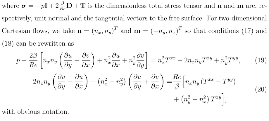
whereσ =−pI+ 2β
ReD+T is the dimensionless total stress tensor andn and mare,
re-spectively, unit normal and the tangential vectors to the free surface. For two-dimensional
Cartesian flows, we take n = (nx, ny)T and m = (−ny, nx)T so that conditions (17) and
(18) can be rewritten as
p− 2β Re
nxny
∂u ∂y + ∂v ∂x +n2x
∂u ∂x +n
2
y
∂v ∂y
=n2xT xx
+ 2nxnyTxy +n2yT yy
, (19)
2nxny
∂v ∂y − ∂u ∂x
+ n2x−n2y
∂u ∂y + ∂v ∂x =Re β h
nxny(Txx−Tyy)
+ n2y −n2x
Txyi,
(20)
with obvious notation.
3. Numerical method
The numerical method used to obtain the solution of the governing equations is based
on the Simplified-Marker-And-Cell formulation [8] (see also [28]) and employs the finite
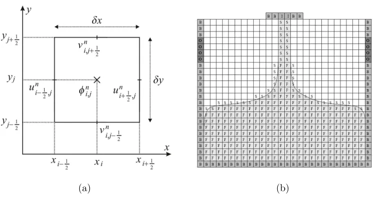
difference method on a staggered grid. Figure 1(a) illustrates an example of a
two-dimensional staggered cell where the velocity components are stored in the middle of the
cell faces while the other variables, represented by the variable φ, are positioned at the
cell centre.
In this work we shall treat flows with moving free surfaces so that a scheme to track
the moving free surface and the fluid region is employed. For this, the cells in the mesh
[image:6.595.69.529.326.534.2](a) (b)
Figure 1: (a) Discrete variables in a staggered cell (i, j) and (b) illustration of cell type classification
used.
• EMPTY (E): cells that do not contain fluid;
• FULL (F): cells that contain fluid and do not have any face in contact with E cell faces;
• SURFACE (S): cells that contain fluid and have one or more faces in contact with
E cell faces;
• INFLOW (I): cells that define an inflow;
• OUTFLOW (O): cells that define an outflow;
• BOUNDARY (B): cells that define the position and location of rigid walls.
This cell classification scheme facilitates the application of the different boundary
condi-tions. Figure 1(b) illustrates this classification for a given instant of time. In this Figure,
for clarity, the E cells are represented by blank cells.
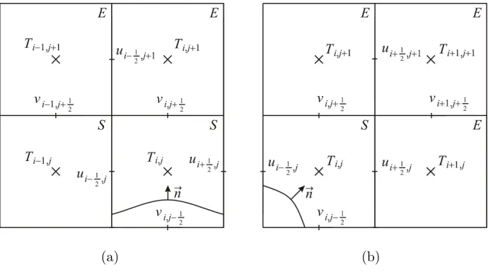
For the application of the boundary conditions at the free surface we follow the ideas
of Tome and McKee [56]. We assume that the mesh is sufficiently fine so that the free
surface can be locally approximated by a linear suface which can be horizontal or vertical
[image:7.595.112.484.118.323.2](a) (b)
Figure 2: Free surface intercepting two opposite faces (a) and two adjacent faces (b) of aScell. In the
case (a), ~n is assumed to be parallel to one of the coordinated axis, and we select~n = (0,1)T. For the
case described in (b), the normal vector~nis assumed to be at an angle of 45o with the coordinate axes,
and we select~n= (√1 2,
1
√
2)
T.
The momentum equation (9) together with the mass conservation equation (1) are
solved by a projection method to uncouple the velocity and pressure fields. The
projec-tion method was originally proposed by Chorin [17], and several modificaprojec-tions have been
presented in the literature (e.g. [13], [27] among many others). However, there are only
a few papers dealing with free surface flows, for instance, [39], [45], [68]. In this paper,
we extend some ideas presented by Oishi et al. [39] for Newtonian free surface flows and
apply these to the solution of the XPP model.
In many applications involving the flow of polymers, the Reynolds number is typically
small (Re <1), at least in parts of the spatial domain. Therefore, to avoid the parabolic
stability restriction inherent in explicit schemes, the momentum equation (9) is integrated
implicitly in time by the Crank-Nicolson method. In this case, the Navier-Stokes equations
(9) and (1) may be rewritten as
u(n+1)−u(n)
δt +∇ ·(uu) (n)
+∇p(n+1) = β 2Re
∇2u(n+1)+∇2u(n)
+∇ ·T(n+12)+ 1
F r2g,
and
∇ ·u(n+1)=0, (22)
where the term ∇ ·T(n+12) is treated as a source term and is calculated by
∇ ·T(n+12) = 1
2 h
∇ ·T(n)+∇ ·T(n+1)i. (23)
The tensor T(n+1) is obtained by solving a hyperbolic equation using a Runge-Kutta method that will be described in Section 3.2. From now on, the upper indices (n) and
(n+ 1) denote the fields at times t=tn and t =tn+δt, respectively.
The projection method based on the Helmholtz-Hodge decomposition (see [23]) states
that every smooth vector field can be decomposed as a sum of a gradient and a
divergence-free vector field, i.e.,
e
u(n+1) =u(n+1)+∇ψ(n+1). (24)
To obtain the intermediate velocityue(n+1), we approximatep(n+1) byp(n) in equation (21) and calculate ue(n+1) from
e
u(n+1)−u(n)
δt +∇ ·(uu) (n)
+∇p(n) = β 2Re
∇2eu(n+1)+∇2u(n)
+∇ ·T(n+12)+ 1
F r2g.
(25)
The boundary conditions for ue are the same as those imposed on u. To enhance the
stability of the Crank-Nicolson method the boundary conditions on rigid walls are dealt
with implicitly (see Oishi et al. [40]).
Once ue(n+1) has been obtained we take the divergence of (24) and, upon imposing mass conservation onu(n+1), we obtain the following Poisson equation for ψ(n+1)
∇2ψ(n+1)=∇ ·eu(n+1). (26)
The boundary conditions required for solving this Poisson equation are the homogeneous
Neumann boundary conditions for rigid walls and inflows while homogeneous Dirichlet
Having solved the Poisson equation (26) forψ(n+1), the final velocityu(n+1)is obtained from equation (24). The pressure is then computed by introducing (24) into (25) and, by
comparing it with equation (21), we obtain the following equation
p(n+1) =p(n)+ψ(n+1) δt −
β
2Re∇
2ψ(n+1). (27)
Once u(n+1) and p(n+1) have been calculated, we are in a position to obtain the non-Newtonian extra-stress tensor Tn+1 through the XPP constitutive equation (see Section 3.2).
3.1. Implicit calculation of the pressure on the free surface
Explicit MAC-type methods for solving a variety of viscoelastic free surface flows have
been presented by Tom´e et al. [55, 58, 59, 60] (see also Paulo et al. [44]). In these papers,
the pressure boundary condition on the free surface has been computed from equation
(19) explicitly so that the boundary condition for the Poisson equation (26) has been
ψ(n+1) = 0 on the free surface cells (Scells). This procedure imposes a parabolic stability restriction on the time step size of the formδt < Re
4 δ
2, whereδis the spatial mesh spacing (assuming a uniform grid). If, however, the problem involves low Reynolds number flow
in any part of the flow region then the CPU time can be considerable. A methodology
that allows one to overcome this often severe restriction for the specific problem of free
surface flows was originally proposed by Oishi et al. [38]: here, the authors presented an
implicit technique for solving low Reynolds number Newtonian flows. More recently, this
idea has been extended to three-dimensional free surface flows (Oldroyd-B [39] and UCM
[61]) and good results were reported. For these reasons, we follow the ideas in [39, 61]
and extend them to solve viscoelastic free surface flows of XPP fluids.
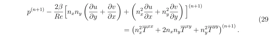
To apply this strategy, we consider two-dimensional free surface flows, and approximate
equation (19) implicitly by
p(n+1)− 2β Re
h
nxny
∂u ∂y + ∂v ∂x +
n2x
∂u ∂x +n
2
y
∂v ∂y
i(n+1)
= n2xTxx + 2n
xnyTxy +n2yT
yy(n+1).
(28)
This equation couples the pressure, velocity and the non-Newtonian extra-stress tensor
field from the velocity and pressure fields by simply substituting T(n+1) by T(n). In this paper, we perform an additional step and compute an approximationT(n+1)by the explicit Euler method. The details of the calculation ofT(n+1) will be given in Section 3.2. Thus, introducing T(n+1) into equation (28) we obtain
p(n+1)
− 2β
Re
h
nxny
∂u ∂y + ∂v ∂x +
n2x
∂u ∂x +n
2
y
∂v ∂y
i(n+1)
= n2xT xx
+ 2nxnyT xy
+n2yT
yy(n+1) .
(29)
To solve this equation we use (24) and (27) to generate new equations for the potential
function on free surface cells which are now coupled with the Poisson equation (26). To
illustrate this strategy, we will show how to obtain the equations for ψ(n+1) for the cases of two free surface orientations. For instance, let us consider the surface cell displayed in
Figure 2(a). For this cell we take n= (0,1)T in which case equation (29) reduces to
p(n+1) = 2β
Re
∂v ∂y
(n+1)
+ (Tyy)(n+1). (30)
Now, imposing mass conservation (22) we get
∂v
∂y
(n+1)
=−∂u
∂x
(n+1)
(31)
and, upon introducing (31) into (30), we obtain
p(n+1) =−2β
Re
∂u ∂x
(n+1)
+ (Tyy)(n+1). (32)
Now, substituting the pressure from equation (27) into (32), we get
p(n)+ ψ (n+1)
δt − β
2Re∇
2ψ(n+1) =
−Re2β
∂u ∂x
(n+1)
+ (Tyy)(n+1). (33)
Finally, from equation (24) we have
u(n+1) =ue(n+1)− ∇ψ(n+1) (34)
which, when introduced into (33), produces the following equation for ψ(n+1):
ψ(n+1) δt −
2β Re
∂2ψ ∂x2
(n+1)
− 2Reβ ∇2ψ(n+1) =−p(n)− 2β
Re
∂eu ∂x
(n+1)
[image:11.595.80.522.210.277.2]Thus, for every free surface cell that has a normal vector defined by n= (0,1)T, we have
obtained one equation for ψ(n+1) associated with that cell.
For the case depicted in Figure 2(b), we approximate the free surface by a 450 sloped surface so that the normal vector is n =√1
2, 1 √ 2
T
. In this case, equation (29) reduces
to
p(n+1) = β
Re ∂u ∂y + ∂v ∂x
(n+1) +1
2 T
xx
+ 2Txy +Tyy(n+1). (36)
We now introduce p(n+1) from (27) and u(n+1) from (24) into equation (36) to obtain
ψ(n+1) δt +
2β Re
∂2ψ(n+1) ∂y ∂x −
β
2Re∇
2ψ(n+1)=−p(n)+ β Re
∂ue ∂y +
∂ev ∂x
(n+1)
+1 2 T
xx
+ 2Txy +Tyy(n+1).
(37)
Again, for each surface cell which possesses the normal vector n = √1 2,
1 √ 2
T
, we have
obtained one equation involving the potentialψ(n+1), associated with that specific cell. For more details of the derivation of other orientations, see Oishi et al. [38].
3.2. Calculation of the non-Newtonian extra-stress tensor for the XPP model
The non-Newtonian stress tensor T for the XPP model is computed from equation
(10) by a second-order Runge-Kutta method as follows. From equation (10), we define
F(u,T) =h(∇u)·T+T·(∇u)Ti+ 2ξD−[∇ ·(uT)]
−W e1
f(λ,T)T+ξ(f(λ,T)−1)I+ α
ξ(T·T)
.
(38)
Then,T(n+1) is obtained in two stages. First, an approximateT(n+1) is calculated by the explicit Euler method, namely,
T(n+1) =T(n)+δtF u(n),T(n). (39)
In the second stage we solve the XPP constitutive equation by the second order modified
Euler method given by
T(n+1) =T(n)+ δt 2
h
F u(n),T(n)+F
u(n+1),T(n+1)
i
To compute equations (39) and (40) the following equations are used:
Fxx(u,T) = 2
∂u ∂xT
xx+ ∂u
∂yT
xy
−
∂(uTxx)
∂x +
∂(vTxx)
∂y
+ 2ξ∂u ∂x −
1
W e
f(λ,T)Txx+ξ(f(λ,T)
−1) +α
ξ
(Txx)2
+ (Txy)2
,
(41)
Fyy(u,T) = 2
∂v ∂xT
xy+ ∂v
∂yT
yy
−
∂(uTyy)
∂x +
∂(vTyy)
∂y
+ 2ξ∂v ∂y −
1
W e
f(λ,T)Tyy +ξ(f(λ,T)
−1) + α
ξ
(Tyy)2
+ (Txy)2
,
(42)
Fxy(u,T) =
∂v ∂xT
xx+ ∂u
∂yT
yy
−
∂(uTxy)
∂x +
∂(vTxy)
∂y +ξ ∂u ∂y + ∂v ∂x
−W e1
f(λ,T)Txy+ α
ξ [T
xy(Txx+Tyy)]
,
(43)
where from (11) we have
f(λ,T) = 2
γ
1− 1
λ
eQ0(λ−1) + 1
λ2
1− α 3ξ2
(Txx)2
+ 2Txy + (Tyy)2
(44)
and
λ= r
1 + 1 3ξ |T
xx+Tyy|. (45)
3.2.1. Computation of the non-Newtonian extra-stress tensor on mesh boundaries
When solving equations (41)-(43) in order to compute T(n+1) from (39) and T(n+1)
from (40), care should be taken when approximating the derivatives contained within
the material derivative of equations (41)-(43). It is known that first order upwinding
can result in solutions that contain excessive diffusion while second order central
differ-ence approximations can lead to oscillatory solutions. To avoid these difficulties many
researchers have been developing high order accurate stable upwind methods to
approx-imate the convective terms of hyperbolic equations. In this work we employ CUBISTA
(Convergent Universally Bounded Interpolation Scheme for the Treatment of Advection)
[7]. This method requires that the values of the variable to be approximated, sayϕ, be
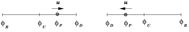
ap-proximated by using upstream (ϕU), downstream (ϕD) and remote upstream (ϕR) values with respect to the point at which the variable is defined (see Figure 3). Therefore, when
further values of the non-Newtonian stress tensor T are needed. These are obtained as
follows:
φ
Pφ
Rφ
Rφ
Uφ
Pφ
Dφ
Dφ
U [image:14.595.120.479.168.230.2]u u
Figure 3: Reference points used for the CUBISTA upwind scheme.
Inflow boundaries: If the velocity at fluid entrance is constant then we follow the
strategy of Crochet et al. [21] (see also Mompean and Deville [36], Tom´e et al. [58]) and
set T=0, while for fully developed flows prescribed by
u(y) = 4Uy L
1− y
L
, v = 0, (46)
we impose the Oldroyd-B profile for T, namely,
Txx = 2W e
Re
1− λ2
λ1
∂u
∂y
2
, Tyy = 0, Txy = 1
Re
1− λ2
λ1
∂u
∂y
. (47)
Outflow boundaries: At fluid exit we employ homogeneous Neumann conditions (see
Mompean [36], Tom´e et al. [58])
∂Txx
∂n = ∂Txy
∂n = ∂Tyy
∂n = 0, (48)
where n denotes the normal direction to the boundary.
Rigid walls: On these boundaries we use the no-slip condition (u=0) and compute T
directly from equation (10). For instance, on a rigid wall parallel to thex-axis the tensor
T is calculated from the equations
∂Txx
∂t = 2 ∂u ∂yT
xy
−W e1 nf(λ,T)Txx+ξf(λ,T)
−1+α
ξ
(Txx)2+ (Txy)2o, (49) ∂Tyy
∂t = −
1
W e
n
f(λ,T)Tyy+ξf(λ,T)
−1+α
ξ
(Txy)2+ (Tyy)2o, (50) ∂Txy
∂t = ∂u ∂y T
yy
+ξ− 1 W e
n
f(λ,T)Txy+ α
ξ
Txy Txx+Tyyo. (51)
The equations for calculating the non-Newtonian extra-stress tensor on rigid walls parallel
3.3. Computational algorithm
We are now in a position to write down the algorithm for simulating the flow of a XPP
fluid. It is supposed that at time t = tn the solenoidal velocity u(n), the pressure field
p(n), the non-Newtonian extra-stress tensor T(n) are known. The solutions u(n+1), p(n+1) and T(n+1) are obtained by the following steps.
1. Compute the stress tensor on mesh boundaries according to the equations described
in Section 3.2.1.
2. Calculate T(n+1) from equation (39) and then compute T(n+1
2) by equation (23).
3. Calculate the intermediate velocity ue(n+1) from equation (25) using the Crank-Nicolson scheme. The resulting linear systems are solved by the Conjugate Gradient
method with diagonal pre-conditioning.
4. Solve the Poisson equation (26) simultaneously with the equations obtained for
ψ(n+1) from the application of the boundary conditions for the pressure on the free surface (see Section 3.1). The corresponding finite difference equations will
generate a large nonsymmetric linear system which can be efficiently solved by the
Bi-conjugate gradient method with SOR (BiCGstab-SOR) pre-conditioning.
5. Calculate the final velocity field u(n+1) from equation (24).
6. Update the final pressure field p(n+1) using equation (27).
7. Calculate T(n+1) using equation (40).
8. Move the free surface. In this last step, the velocity u(n+1) is used to compute a new free surface by solving
dxP
dt =u (n+1)
P (52)
employed. Details on the free surface movement and particle insertion/deletion can
be found in Tom´e et al. [57].
The approximation of the equations contained in the algorithm above by the finite
dif-ference method is a somewhat obvious extention of those in [58] and so are not given
here.
4. Time-step calculation
The Oldroyd-B solver of Tom´e et al. [58] solves the momentum equation explicitly so
that the time-step size is required to satisfy the restrictions
δt < δtV ISC =
Re
4 h
2, (53)
δt < δtCF L =
h Vmax
, (54)
where Vmax denotes the maximum of velocity in the x and y−directions. Condition (53)
is a viscous restriction due to the explicit calculation of the momentum equations while
(54) is the CFL condition. Therefore, if the Reynolds number is small (Re << 1) then
condition (53) would lead to a very small time-step. One reason the Crank-Nicolson is
being employed to solve the momentum equations is that we expect it to obey a less
restrictive condition. We follow the procedure employed by Oishi et al. [39] (see also
Tome and McKee [56]) and compute the time step by
δt=f act∗minf act1∗δtV ISC, f act2∗δtCF L (55)
where f act, f act1, f act2 > 0. The constants f act, f act1, f act2 appear as a conservative measure since the true solenoidal velocities are not known at the begining of the
calcu-lation. The implementation of these inequalities follows the ideas of Tome and McKee
[56].
In the calculations presented by the explicit Oldroyd-B solver of Tom´e et al. [58] the
constantf actassumed the value of 0.2 while the constants f act1 andf act2 were assigned the value of 0.5. However, if the flow involves a low Reynolds number (Re << 1) then
Oishi et al. [39] and set the value of the constant f act1 >>1; for instance, in this paper we use f act1 = 10. This more than compensates for the extra computations arising from using the Crank-Nicolson method to solve the momentum equations.
5. Verification of the numerical method
To verify the correctness of the numerical method presented in this paper, we simulated
the flow of a XPP fluid in a two-dimensional channel of width L and length 5L. At the
channel entrance, the fully developed flow given by equation (46) was used while the
non-Newtonian extra-stress tensorT assumed the Oldroyd-B profile of equation (47). At
the channel exit a homogeneous Neumann condition was imposed for both the velocity
and the non-Newtonian extra-stress tensor T. At the channel walls the velocity obeyed
the no-slip condition while the non-Newtonian extra-stress tensor T was calculated from
equations (49)-(51).
The simulation started with the channel empty. Fluid was then injected through the
entrance and the channel progressively filled. Initially, there was a free surface within the
channel and on that free surface the boundary conditions imposed were the free surface
stress conditions given by equations (19) and (20).
The following input data were employed: L = 1, U = 1, Re= 0.1, W e= 2, β = 0.5,
α = 0.2, γ = 0.5, Q = 2.0 and gravity was neglected. To study the convergence of the
numerical method, channel flow was simulated on five meshes: M1 (h= 0.2, 5×25 cells),
M2 (h= 0.1,10×50 cells), M3 (h= 0.05, 20×100 cells), M4 (h= 0.025, 40×200 cells)
and M5 (h= 0.0125, 80×400 cells). An analytic solution for this problem is not known
so we compared the numerical solutions obtained on meshes M1, M2, M3 and M4 to the
solution obtained on mesh M5 which, hereafter, we shall refer to as SOLEXACT.
Channel flow was simulated on the meshes mentioned above untilt = 50. At this time
the results did not show any variation implying that steady state had been established.
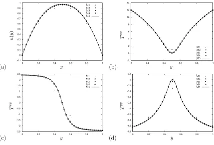
The solution profiles obtained by the numerical method using the meshes mentioned
above are displayed in Figure 4 where we can observe that the solutions obtained on meshes
numerical method we calculated the relative errors using the l2-norm by
kEk2 =
sP
i,j(SOLEXACT −SOLN U M)2
P
i,j(SOLEXACT)2
(56)
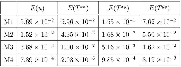
whereSOLN U M denotes the solutions obtained on meshes M1 to M4. Table 1 displays the
calculated errors for the velocity u and also for the components of the tensor T. We can
see in Table 1 that as the mesh is refined all the errors decreased indicating convergence
[image:18.595.143.456.328.445.2]of the algorithm.
Table 1: Errors obtained on meshes M1, M2, M3 and M4.
E(u) E(Txx) E(Txy) E(Tyy)
M1 5.69×10⁻² 5.96×10⁻² 1.55×10⁻¹ 7.62×10⁻² M2 1.52×10⁻² 4.35
×10−2 1.68
×10−2 5.50
×10−2
M3 3.68×10⁻³ 1.00×10⁻² 5.16×10⁻³ 1.62×10⁻² M4 7.39×10⁻⁴ 2.03×10⁻³ 9.85×10⁻⁴ 3.19×10⁻³
5.1. The convergence of the free surface
To supply further evidence concerning the convergence of the numerical method, we
simulated the time-dependent extrudate swell problem (for details see Section 6) using
[image:18.595.143.457.330.446.2]three meshes: M1 (h = 0.1), M2 (h = 0.05) and M3 (h = 0.025). With reference to
Figure 5 we used L= 1; the velocity at the channel entrance was given by equation (46)
with U = 1 while the non-Newtonian extra-stress tensor T was defined by equation (47).
In this study we considered the XPP model with the following parameters: α = 0.1,
Re= 0.05,W e= 10, β = 0.5,γ = 0.8, Q= 8.0.
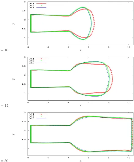
The fluid surface obtained in these simulations at times t = 10, t = 15 and t = 50
are displayed in Figure 6. From this Figure, we can observe that the free surface profiles
obtained on meshes M1 and M2 approach the free surface profile obtained using the
finer mesh M3. This result indicates the convergence of the numerical method for
(a) -0.1 0 0.1 0.2 0.3 0.4 0.5 0.6 0.7 0.8 0.9 1
0 0.2 0.4 0.6 0.8 1 M1 M2 M3 M4 M5 y u ( y ) (b) -2 0 2 4 6 8 10 12 14
0 0.2 0.4 0.6 0.8 1
M1 M2 M3 M4 M5 y T x x (c) -2.5 -2 -1.5 -1 -0.5 0 0.5 1 1.5 2 2.5
0 0.2 0.4 0.6 0.8 1 M1 M2 M3 M4 M5 y T x y (d) -1.8 -1.6 -1.4 -1.2 -1 -0.8 -0.6 -0.4 -0.2 0 0.2
[image:19.595.82.511.124.415.2]0 0.2 0.4 0.6 0.8 1 M1 M2 M3 M4 M5 y T y y
Figure 4: Numerical solution of channel flow of a XPP fluid. Comparison of the numerical solutions
obtained on meshes M1, M2, M3 and M4 with the numerical solution obtained on mesh M5. (a)u, (b)
Txx, (c)Txy, (d)Tyy.
In addition, a comparison was performed between the spectral method of Russo and
Phillips [50] and the Marker and Cell approach of this paper. The extrudate swell problem
was simulated for the XPP model with the following parameters: α= 0.025, Re= 1, W e=
1, β = 0.11111111, γ = 1.0 and Q= 4.0. The domain over which the problem was solved
was the same as that used by Russo and Phillips [50] with the die exit at (nondimensional)
x = 20. One can see from Figure 7 that the profile of the free surface obtained by the
method of this paper exhibits similar qualitative behaviour. Since the non-dimensional
scaling in the Russo and Phillips paper is not specified, and the two methods are quite
different, these results, we would argue, are quite good and display reasonable qualitative
L L max
x y
6L L
L
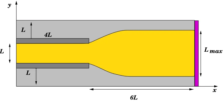
[image:20.595.116.481.123.293.2]4L
Figure 5: Domain definition for the simulation of unsteady extrudate swell (pink surface represents an
outflow boundary through which the fluid can flow).
5.2. Efficiency of the linear solvers
In this work, two linear solvers were employed: the Conjugate Gradient method with
diagonal pre-conditioning or Jacobi pre-conditioner (CG-Jacobi) and the Bi-Conjugate
Gradient Stabilized with a SOR pre-conditioner (BiCGstab-SOR). The CG-Jacobi was
used to solve the symmetric linear system resulting from the discretization of the
momen-tum equations for calculating the intermediate velocity eu(n+1) while the BiCGstab-SOR was applied to invert the nonsymmetric linear system to obtain the pressure ψ (see the
computational algorithm in the Section 3.3).
To illustrate the effect of grid refinement for solving the extrudate swell problem, we
report in Table 2 a study on the efficiency of the preconditioners for three meshes: M1,
M2 and M3 (see Section 5.1). Table 2 displays the number of equations (Neq(·)) forue(ue
and ve) and ψ, the number of iterations (Nit(·)), and the rate of increase in the number
of iterations compared to the increase in the number o equations which is estimated from
the following equation:
Ni(·) =
T it(Mi+1)/T it(Mi)
T eq(Mi+1)/T eq(Mi)
, i= 1,2. (57)
In equation (57) we define T eq and T it as, respectively, the total numbers of equations
t= 10
1 1.5 2 2.5 3
0 2 4 6 8 10
M1 M2 M3
x
y
t= 15
1 1.5 2 2.5 3
0 2 4 6 8 10
M1 M2 M3
x
y
t= 50
1 1.5 2 2.5 3
0 2 4 6 8 10
M1 M2 M3
x
[image:21.595.77.515.148.678.2]y
Figure 6: Free surface profiles obtained in the simulation of the time-dependent extrudate swell using
the XPP model. Results shown on meshes M1, M2 and M3 at selected times. XPP model parameters
2 2.2 2.4 2.6 2.8 3 3.2 3.4
20 21 22 23 24 25 26 27 28 29
PRESENT WORK RUSSO and PHILLIPS
x
[image:22.595.126.467.130.375.2]y
Figure 7: Comparison between present computation and the numerical method of Russo and Phillips [50]
for the time-dependent extrudate swell using the XPP model.
To simplify our study, we chose a specific model by setting α= 0.1,Re= 0.05,W e= 10,
β = 0.5, γ = 0.8, Q= 8.0.
It is evident from this table that the preconditioners Jacobi, for calculating ue, and
SOR, to solve the nonsymmetric linear system for ψ, are sensitive to the number of
equations, and the number of iterations increases as the grid is refined.
In particular, we see that the number of iterations appears to increase linearly with
the number of equations. From Table 2 we observe that the number of equations for
mesh M2 is roughly 4 times that of M1 and the number of equations for mesh M3 is again
roughly 4 times that of M2. This is so for the linear system arising from the discretization
of the momentum equations (ue - column 2 of Table 2 ) as well as for the linear system
arising from the discretization of the equation to obtain the pressure ψ (column 5 of
Table 2). As for the number of iterations we see from columns 3 and 6 of Table 2 that
this number doubles with each mesh refinement. In columns 4 and 7 we present the
ratio calculated from (57) which show that the iteration count increases linearly with the
To study the efficiency of these solvers we present in Table 3 a comparison between
the solvers employed in this work and the solvers used in our previous work (see [39, 61])
for the extrudate swell problem. We simulated the extrudate swell using the same domain
and mesh M3 employed in Section 5.1.
We considered the solution at time t = 45s and displayed, in Table 3, the number of
iterations taken by the linear solvers as well as the total CPU time of the entire simulation.
From Table 3 we can see that for the CG-Jacobi, the number of iterations required for
the solution of the linear systems for eu and ev was slightly smaller than the number of
iterations taken by the CG without pre-conditioning. Thus, in this case the use of a simple
pre-conditioner led to modestly improved convergence. On the other hand, Table 3 shows
that the number of iterations required by the preconditioned BiCGstab-SOR to solve
the nonsymmetric linear system was remarkably reduced when compared with the
BiCG-Jacobi method. Therefore, the application of an efficient pre-conditioner to reduce the
number of iterations for solving the nonsymmetrical linear system was essential. Finally,
Table 3 shows that the CPU time taken using the solvers CG-Jacobi/BiCGstab-SOR was
substantially less than the CPU time for the solvers CG/BiCG-Jacobi.
In these numerical experiments, the convergence criterion for the linear solvers was
ǫ = 10−10 while the relaxation parameter in the SOR pre-conditioner was ω = 1.8. The results were obtained on a computer with 4 × AMD Opteron 844 / 1.8 GHz processor
and 8 Gbytes RAM running Linux.
Table 2: Influence of mesh refinament on CG-Jacobi/BiCGstab-SOR methods for solving the extrudate
swell problem.
Mesh N eq(ue) N it(eu) Ni(ue) N eq(ψ) N it(ψ) Ni(ψ)
M1 3234 31 − 1698 13 −
M2 13224 66 0.52 6674 24 0.47
Table 3: Performance study of the linear solvers employed in the implicit methodology. Input data used:
α= 0.1,Re= 0.05,W e= 10,β= 0.5,γ= 0.8,Q= 8.0.
Methods N it(ue) N it(ψ) CPU time
(in hours)
CG/BiCG-Jacobi 154 597 50.4
CG-Jacobi/BiCGstab-SOR 126 44 18.1
Table 4: Influence of mesh refinament on CG/BiCG-Jacobi methods for solving the extrudate swell
problem.
Mesh N eq(ue) N it(eu) Ni(ue) N eq(ψ) N it(ψ) Ni(ψ)
M1 3234 32 − 1698 73 −
M2 13224 66 0.52 6674 180 0.62
6. Numerical simulation of unsteady extrudate swell
The unsteady extrudate swell problem consists of a jet of viscous fluid exiting a
cap-illary of width L where, due to the normal stress differences, the jet swells and its width
expands to a maximum Lmax (see Figure 5). The amount of swell can be measured by
computing the swelling ratio Sr given by
Sr =
Lmax
L . (58)
It is known that for Newtonian fluids, the jet does not suffer large swelling ratios and for
low Reynolds number axisymmetric jets the maximum Sr is of order 13% (see Bird et al.
[10]). However, for viscoelastic fluids, the jet swell can be very large and the swelling ratio
Sr can attain values above 100% (e.g. [19]). This problem has many applications so that
considerable effort has been employed to develop techniques to simulate the extrudate
swell of complex fluids (e.g. [20, 44, 50, 53, 55, 58]).
To demonstrate that the implicit technique presented in this paper can cope with the
complex flows obtained from using the Pom-Pom model we applied it to simulate this
unsteady extrudate swell problem.
We considered a 2D-channel with width L and length 4L and an outflow boundary
positioned at a distance 6Lfrom the channel exit. A domain size of 10L×3Lwas employed
(see Figure 5). On the channel entrance, walls and outflow, the boundary conditions were
the same as those employed in the previous section. On the moving free surface, the
boundary conditions were those described in Section 2.1, namely (19) and (20).
In the results presented next, we employed L= 1, U = 1, Re= 0.05 and used a mesh
spacing h = 0.05 in all simulations. As the Reynolds number is small (Re << 1) we
anticipate that a length of 3L was sufficient for the flow to develop inside the channel.
The time step was automatically generated subject to the restrictions given in Section 4.
To verify the robustness of the numerical method we investigated the effect of the
Pom-Pom parameters on the extrudate swelling ratio (Sr). We perfomed a number of
6.1. Influence of α
The extrudate swell depends on the first normal stress difference (N1) while in the XPP model the parameterαis the coefficient in front of the second normal stress difference (N2). Therefore, we might anticipate that the smaller the parameter α is, the greater would be
the swelling ratioSr. To verify this hypothesis we simulated the unsteady extrudate swell
for increasing values of the parameter α while the remaining parameters were held fixed.
We used W e = 10,β = 0.5, γ = 0.8,Q = 8.0 and α= 0.0, 0.05, 0.1, 0.2, 0.4, 0.6, 0.8.
Figure 8 displays the fluid flow visualization at selected times while Figure 9 shows the
variation of the extrudate swelling ratio (Sr) as function of α. We can see from Figure
9 that the extrudate swelling decreases as α increases; the maximum swelling ratio was
approximately 2.15 forα= 0 and the smallest swelling ratio was approximately 1.35 when
α= 0.8. Despite a high Weissenberg number (W e = 10), we note that the swelling ratio
was rather modest when α = 0.8.
α= 0.0
α= 0.1
α= 0.2
α= 0.4
α= 0.8
[image:26.595.73.519.431.680.2]t= 10s t= 15s t = 50s
Figure 8: Numerical simulation for the extrudate swell of a XPP fluid using the implicit formulation.
Fluid flow visualization for different values ofαat selected times. Re= 0.05,W e= 10,β = 0.5,γ= 0.8,
1.3 1.4 1.5 1.6 1.7 1.8 1.9 2 2.1 2.2
0 0.1 0.2 0.3 0.4 0.5 0.6 0.7 0.8
[image:27.595.120.474.126.382.2]α Sr
Figure 9: Extrudate swelling ratiosSrobtained as function of α.
6.2. Influence of β
The parameter 0≤β ≤1 is associated with the amount of Newtonian solvent. A value
of β close to zero corresponds to highly entangled systems (highly elastic fluids) while a
value of β near 1 corresponds to dilute or less-entangled solutions (almost a Newtonian
fluid). More details about the significance of the parameter β in the XPP model can be
found in Aboubacar et al. [3].
To analyze the influence of the solvent contribution on the swelling ratio Sr, the
ex-trudate swell was simulated using the following data: β = 0.2, 0.4, 0.6, 0.8, 0.9 and
W e = 10.0, α = 0.01,γ = 0.3, Q= 8.0. Figure 10 illustrates the fluid flow visualization
obtained for different values of β. We observe that the extrudate swelling ratio increases
when the polymeric solution becomes more concentrated as we can see clearly from Figure
11. Indeed, we observe that Sr is decreasing linearly when β > 0.4. Thus, the largest
extrudate swelling ratio was obtained for the smallest value of β employed. Conversely,
β = 0.2
β = 0.4
β = 0.6
β = 0.8
β = 0.9
[image:28.595.81.518.126.371.2]t= 10s t= 15s t = 50s
Figure 10: Numerical simulation for the extrudate swell of a XPP fluid using the implicit formulation.
Fluid flow visualization for different values ofβat selected times. Re= 0.05,W e= 10,α= 0.01,γ= 0.3,
Q= 8.
1.1 1.2 1.3 1.4 1.5 1.6 1.7 1.8
0.2 0.3 0.4 0.5 0.6 0.7 0.8 0.9
β Sr
[image:28.595.119.471.463.725.2]6.3. Influence of γ
In the XPP model, the parameter 0 ≤γ ≤ 1 represents the ratio between the
relax-ation time of the stretch of the backbone (λ1) and the orientation relaxation time (λ2). Thus, this parameter is related to the degree of entanglement of the melt. High values of
γ corresponds to molecules with relatively short backbone lengths while small values of γ
corresponds to highly entangled backbone configurations.
To investigate the influence of γ ∈ (0,1) on the extrudate swelling ratio of a XPP
fluid we performed a number of simulations of unsteady extrudate swell for various values
of γ. The parameters W e = 10, α = 0.01, β = 0.5, Q = 8.0 were kept fixed while the
parameter γ assumed the following values 0.2, 0.25, 0.4, 0.6, 0.8, 0.9.
Figure 12 displays the time evolution of the extrudate swell for each value of γ. We
can see that asγ increases the extrudate swell also increases. This is quantified in Figure
13 where the extrudate swelling ratios are given as a function of γ. We note that for
γ ∈ [0,0.6] the extrudate swelling ratioSr grows linearly and monotonically withγ. In
γ = 0.2
γ = 0.25
γ = 0.4
γ = 0.6
γ = 0.9
[image:30.595.80.519.125.371.2]t= 10s t= 15s t = 50s
Figure 12: Numerical simulation for the extrudate swell of a XPP fluid using the implicit formulation.
Fluid flow visualization for different values ofγat selected times. Re= 0.05,W e= 10,α= 0.01,β= 0.5,
Q= 8.0.
1.3 1.4 1.5 1.6 1.7 1.8 1.9 2 2.1
0.2 0.3 0.4 0.5 0.6 0.7 0.8 0.9
γ Sr
[image:30.595.119.471.464.725.2]6.4. Influence of Q
The parameter Q represents the number of arms at each end of the backbone of the
polymeric Pom-Pom molecule and consequently affects the level of entanglement. Thus
one might expect the level of entanglement to become larger with increasing Q.
To investigate the effect of this parameter on the extrudate swell we performed various
simulations with increasing values of Q. The data employed were W e = 10, α = 0.01,
β = 0.5, γ = 0.3, and Q= 1, 2, 4, 7, 11, 15, 20.
The numerical results obtained are summarized in Figures 14 and 15. The fluid flow
visualization of the results at selected times is shown in Figure 14 while Figure 15 displays
the extrudate swelling ratio Sr obtained with the implicit technique described in this
paper. It can be seen in Figure 15 that the extrudate swelling ratio increases as the
number of arms grows.
Q= 1.0
Q= 4.0
Q= 11.0
Q= 15.0
Q= 20.0
[image:31.595.72.523.393.636.2]t= 10s t= 15s t = 50s
Figure 14: Numerical simulation for the extrudate swelling of a XPP fluid using the implicit formulation.
Fluid flow visualization for different values of Q at selected times. Re = 0.05, W e = 10, α = 0.01,
1.4 1.5 1.6 1.7 1.8 1.9 2
2 4 6 8 10 12 14 16 18 20
[image:32.595.122.472.124.381.2]Q Sr
Figure 15: Extrudate swelling ratioSras a function of Q.
6.5. Influence of W e
We now examine the influence of the Weissenberg number on the extrudate swelling
ratio of XPP fluids. This parameter is related to the viscoelasticity of the fluid and it is
anticipated that the extrudate swelling ratio might well be an increasing function ofW e.
To verify this fact, we simulated the time-dependent extrudate swell for the following
values of W e: 0.5, 1, 2, 4, 7, 11, 15, 20.
The results of these simulations are given in Figures 16 and 17. Figure 16 displays the
fluid flow configuration at selected times while Figure 17 plots the swelling ratio obtained
in these simulations. We can see from Figure 17 that the swelling ratio is, indeed, an
W e = 0.5
W e = 2.0
W e = 7.0
W e= 15
W e= 20
[image:33.595.72.524.129.370.2]t= 10s t= 15s t = 50s
Figure 16: Numerical simulation for the extrudate swell of a XPP fluid using the implicit formulation.
Fluid flow visualization for different values of W e at selected times. Re = 0.05, α = 0.01, β = 0.5,
γ= 0.8,Q= 8.0.
1.3 1.4 1.5 1.6 1.7 1.8 1.9 2 2.1 2.2 2.3
2 4 6 8 10 12 14 16 18 20
W e Sr
[image:33.595.120.476.462.721.2]7. Simulation of the Barus effect: the influence of viscosity
The study in the previous section provided some indication as to how the various
parameters might be chosen so that substantial elastic effects might be exhibited. This
section is concerned with finding a particular selection of parameters which will not only
provide a large swelling ratio, but will also (when gravity is included) produce the
so-called Barus effect [29]. This is an elastic memory effect which reduces the swelling ratio,
beyond the capillary outlet, to the original diameter (or even less) of the fluid when it
was flowing in the tube.
On this occasion we have employed a channel of length 10Lthrough which fluid flows
(cf. Figure 5 with 3Lreplaced by 4Land 10Lreplaced by 12L); the length 10Lwas chosen
to ensure steady state flow for a range of Reynolds numbers prior to the emergence of
the jet. The jet then travels a distance of 12L before reaching an outflow (displayed in
pink where continuative outflow boundary conditions are applied). Gravity acts vertically
downwards with g = 9.81ms−2. A mesh size of (40×220)-cells was used (h = 0.1). The data employed in the XPP model are displayed in Table 5. The scaling for the velocity
was U = 0.5ms−1 and the length scale was L= 0.01m.
To observe the influence of viscosity on the Barus effect we performed five simulations
with the Reynolds number taking the values of 0.2, 0.1, 0.05, 0.025 and 0.01. We have
also performed five additional simulations using the same input data except that gravity
has now been set to zero. The difference in Figure 17 is substantial and perhaps a
little surprising. For zero gravity, and the special choice of parameters adduced from the
previous section, the swelling ratio is indeed large and is independent of the Reynolds
number. This is not the case when we switch gravity on. As the Reynolds increases
(but still remains very small) we observe that the swelling ratios are greatly reduced,
as can be seen from the fluid flow visualizations in Figures 19, 20 and 21. To avoid
short wavelenght pertubations on th free surface in this simulation we employed a filter
Table 5: Data used in the XPP model to simulate the Barus effect with gravity.
α β γ Q W e
0.01 0.55 0.8 15 20
1.2 1.4 1.6 1.8 2 2.2 2.4 2.6
0.025 0.05 0.1 0.2
Sr
[image:35.595.129.461.419.656.2]Re
Figure 18: Variation of the swelling ratio Sr againstRe. With gravity (squares) and without gravity
Re= 0.20 Re= 0.10 Re= 0.05 Re= 0.025 Re= 0.01
Figure 19: Numerical simulation of the Barus effect with gravity included. Fluid flow visualization at
Re= 0.20 Re= 0.10 Re= 0.05 Re= 0.025 Re= 0.01
Figure 20: Numerical simulation of the Barus effect with gravity included. Fluid flow visualization at
Re= 0.20 Re= 0.10 Re= 0.05 Re= 0.025 Re= 0.01
Figure 21: Numerical simulation of the Barus effect with gravity included. Fluid flow visualization after
the jet has entered the outflow boundary. Results shown at times: t = 0.78s (Re = 0.20), t = 0.88s
8. Concluding remarks
This work has been concerned with an implicit numerical technique for simulating
two-dimensional viscoelastic free surface flows. The viscoelastic model employed was
the eXtended Pom Pom (XPP) model. The solution strategy for the flow equations
(conservation of mass and momentum) was essentially based on a projection method.
First the equations were nondimensionalised. An intermediate fluid velocity was
cal-culated by a Crank-Nicolson scheme and the resulting linear system solved by conjugate
gradients with a diagonal preconditioner. A Poisson equation using implicit boundary
conditions was solved for a velocity potential which then allowed the divergence free
up-dated velocity to be calculated. The non-Newtonian extra-stress tensor was calculated
by a second order Runge-Kutta method employing this updated velocity. An updated
pressure was then able to be calculated explicitly. Finally, the new position of the moving
free surface, defined by the virtual marker particles, was obtained by solving dxp dt = up
using Euler’s method for each particle.
The algorithm was partially validated by solving channel flow on five different meshes
and results, showing the convergence of the free surface location, were presented by
sim-ulating extrudate swell using mesh refinement. Extrudate swell from a capillary was then
computed and a reasonably comprehensive sensitivity analysis was performed on all the
parameters that characterize the XPP model to determine how they influence the
extru-date swelling ratio. Results were obtained for Weissenberg numbers up to 20, but the code
appeared to suffer from numerical instability thereafter. Finally, armed with this
knowl-edge, we were able to exhibit the Barus effect when the swelling jet is subject to gravity
effects in the direction of the flow; we also showed that gravity could play a significant
role in reducing the swelling ratio.
9. Acknowledgments
We gratefully acknowledge the support from the Brazilian funding agencies: FAPESP
2009/15892−9), CNPq - Conselho Nacional de Desenvolvimento Cient´ıfico e Tecnol´ogico
(grants Nos. 304422/2007−0, 470764/2007−4, 477858/2009−0). This work was
car-ried out in the framework of the Instituto Nacional de Ciˆencia e Tecnologia em Medicina
Assistida por Computa¸c˜ao Cient´ıfica (CNPq, Brazil). The last named author would like
to acknowledge a travel grant from the Royal Society of Edinburgh.
References
[1] M. Aboubacar, H. Matallah, H. R. Tamaddon-Jahromi, and M. F. Webster, Highly
elastic solutions for Oldroyd-B and Phan-Thien/Tanner fluids with a finite
vol-ume/element method: planar contraction flows, J. Non-Newton. Fluid Mech. 103
(2002), pp. 65-103.
[2] M. Aboubacar, H.R. Tamaddon-Jahromi, and M.F. Webster, Time-dependent
algo-rithms for viscoelastic flow: bridge between finite-volume and finite-element
method-ology,Second MIT Conference on Computational Fluid and Solid Mechanics, (2003),
pp. 815-818.
[3] M. Aboubacar, J.P. Aguayo, P.M. Phillips, T.N. Phillips, H.R. Tamaddon-Jahromi,
B.A. Snigerev, and M.F. Webster, Modelling pom-pom type models with high-order
finite volume schemes, J. Non-Newton. Fluid Mech. 126 (2005), pp. 207-220.
[4] A. Afonso, P.J. Oliveira, F.T. Pinho, and M.A. Alves, The log-conformation tensor
approach in the finite-volume method framework, J. Non-Newton. Fluid Mech. 157
(2009), pp. 55-65.
[5] J.P. Aguayo, H.R. Tamaddon-Jahromi, and M.F. Webster, Extensional response of
the pom-pom model through planar contraction flows for branched polymer melts,
J. Non-Newton. Fluid Mech. 134 (2006), pp. 105-126.
[6] J.P. Aguayo, P.M. Phillips, T.N. Phillips, H.R. Tamaddon-Jahromi, B.A. Snigerev,
using the pom-pom model and higher-order finite volume schemes, J. Comput. Phys.
220 (2007), pp. 586-611.
[7] M.A. Alves, P.J. Oliveira, and F.T. Pinho, A convergent and universally bounded
interpolation scheme for the treatment of advection, Intern. J. Numer. Meth. Fluids
41 (2003), pp. 47-75.
[8] A.A. Amsden and F.H. Harlow, A simplified MAC technique for incompressible fluid
flow calculations, J. Comput. Phys. 6 (1970), pp. 332–335.
[9] G.K. Batchelor,An Introduction to Fluid Dynamics, Cambridge, 1970.
[10] R.B. Bird, R.C. Armstrong, O. Hassager, Dynamics of polymeric liquids, Vol I,
Wil-ley, 1987.
[11] G.B. Bishko, O.G. Harlen, T.C.B. McLeish, and T.M. Nicholson, Numerical
simu-lation of the transient flow of branched polymer melts through a planar contraction
using the Pom-Pom model, J. Non-Newton. Fluid Mech. 82 (1999), pp. 255-273.
[12] A. Bonito, M. Picasso, and M. Laso, Numerical simulation of 3D viscoelastic flows
with free surfaces, J. Comput. Phys. 215 (2006), pp. 691-716.
[13] D.L. Brown, R. Cortez, and M.L. Minion, Accurate projection methods for the
in-compressible Navier-Stokes equations, J. Comput. Phys.168 (2001), pp. 464-499.
[14] G.C. Buscaglia, A finite element analysis of rubber coextrusion using a power-law
model, Intern. J. Numer. Meth. Eng. 36 (1993), pp. 2143-2156.
[15] Z. Cai and C.R. Westphal, An adaptive mixed least-squares finite element method
for viscoelastic fluids of Oldroyd type, J. Non-Newton. Fluid Mech.159 (2009), pp.
72-80.
[16] H.C. Choi, J.H. Song and J.Y. Yoo, Numerical-Simulation of the Planar Contraction
[17] A.J. Chorin, Numerical solution of the Navier-Stokes equations, J. Comput. Phys.2
(1968), pp. 745-762.
[18] N. Clemeur, R.P.G. Rutgers, and B. Debbaut, On the evaluation of some differential
formulations for the pom-pom constitutive model, Rheol. Acta, 42 (2003), pp.
217-231.
[19] M. Cloitre, T. Hall, C. Mata, and D.D. Joseph, Delayed-die swell and sedimentation
of elongated particles in wormlike micellar solutions,J. Non-Newton. Fluid Mech.79
(1998), pp. 157-171.
[20] M.J. Crochet and R. Keunings, Finite element analysis of die-swell of a highly elastic
fluid, J. Non-Newton. Fluid Mech. 10 (1982), pp. 339-356 .
[21] M.J. Crochet, A.R. Davies, and K. Walters,Numerical Simulation of Non-Newtonian
Flow, Elsevier, Amsterdam, 1984.
[22] H. Demir, Numerical modelling of viscoelastic cavity driven flow using finite difference
simulations, Appl. Math. Comput. 166 (2005), pp. 64-83.
[23] F.M. Denaro, On the applications of the Helmholtz-Hodge decomposition in
projec-tion methods for incompressible flows with general boundary condiprojec-tions, Intern. J.
Numer. Meth. Fluids 43 (2003), pp. 43-69.
[24] Y. Fan, R.I. Tanner, and N. Phan-Thien, Galerkin/least-square finite-element
meth-ods for steady viscoelastic flows,J. Non-Newton. Fluid Mech.84(1995), pp. 233-256.
[25] J. Fang, R.G. Owens, L. Tacher, and A. Parriaux, A numerical study of the SPH
method for simulating transient viscoelastic free surface flows, J. Non-Newton. Fluid
Mech. 139 (2006), pp. 68-84.
[26] V. Ganvir, A. Lele, R. Thaokar, and B.P. Gautham, Simulation of viscoelastic flows
of polymer solutions in abrupt contractions using an arbitrary Lagrangian Eulerian
(ALE) based finite element method, J. Non-Newton. Fluid Mech. 143 (2007), pp.
[27] J.L. Guermond, P. Minev, and J. Shen, An overview of projection methods for
in-compressible flows, Comput. Method Appl. M. 195 (2006), pp. 6011-6045.
[28] F.H. Harlow and J.E. Welch, Numerical calculation of time-dependent viscous
in-compressible flow of fluid with free surface, Phys. Fluids 8 (1965), pp. 2182-2189.
[29] I. Hori and S. Okubo, On the normal stress effect and the Barus effect of polymer
melts, J. Rheol. 24 (1980), pp. 39-53.
[30] N.J. Inkson, T.C.B. McLeish, O.G. Harlen, and D.J. Groves, Predicting low density
polyethylene melt rheology in elongational and shear flows with ”pom-pom”
consti-tutive equations, J. Rheol. 43 (1999), pp. 873-896.
[31] N.J. Inkson, T.N. Phillips, and R.G.M. van Os, Numerical simulation of flow past
a cylinder using models of XPP type, J. Non-Newton. Fluid Mech. 156 (2009), pp.
7-20.
[32] R. Keunings and M.J. Crochet, Numerical simulation of the flow of a viscoelastic
fluid through an abrupt contraction, J. Non-Newton. Fluid Mech. 14 (1984), pp.
279-299.
[33] J.M. Kim, C. Kim, J.H. Kim, C. Chung, K.H. Ahn, and S.J. Lee, High-resolution
finite element simulation of 4:1 planar contraction flow of viscoelastic fluid, J.
Non-Newton. Fluid Mech. 129 (2005), pp. 23-37.
[34] X.L. Luo and R.I. Tanner, A Streamline Element Scheme for Solving Viscoelastic
Flow Problems. Differential Constitutive-Equations, J. Non-Newton. Fluid Mech.21
(1989), pp. 179-199.
[35] T.C.B. McLeish and R.G. Larson, Molecular Constitutive Equations for a Class of
Branched Polymers: the Pom-Pom Polymer, J. Rheol. 42 (1998), pp. 81-110.
[36] G. Mompean and M. Deville, Unsteady finite volume simulation of Oldroyd-B fluid
through a three-dimensional planar contraction, J. Non-Newton. Fluid Mech. 72
[37] N. Mangiavacchi, A. Castelo, M.F. Tom´e, J.A. Cuminato, M.L.B. de Oliveira, and
S. McKee, An effective implementantion of surface tension using Marker and Cell
method for axisymmetric and planar flows, SIAM J. Sci. Comput. 26 (2005), pp.
1340-1368.
[38] C.M. Oishi, J.A. Cuminato, V.G. Ferreira, M.F. Tom´e A. Castelo, N. Mangiavacchi,
and S. McKee, A stable semi-implicit method for free surface flows, Trans. ASME J.
Appl. Mech. 73 (2006), pp. 940–947.
[39] C.M. Oishi, M.F. Tom´e, J.A. Cuminato, and S. McKee, An implicit technique for
solving 3D low Reynolds number moving free surface flows, J. Comput. Phys. 227
(2008), pp. 7446-7468.
[40] C.M. Oishi, J.A. Cuminato, J.Y Yuan, and S. McKee, Stability of numerical schemes
on staggered grids, Numer. Lin. Alg. Applics. 15 (2008), pp. 945-967.
[41] P.J. Oliveira, F.T. Pinho, and G.A. Pinto, Numerical simulation of non-linear elastic
flows with a general collocated finite-volume method, J. Non-Newton. Fluid Mech.
79 (1998), pp. 1-43.
[42] R.G. Owens and T.N. Phillips, Computational Rheology, World Scientific Publishing
Company, 2002.
[43] M. Pasquali and L.E. Scriven, Free surface flows of polymer solutions with models
based on the conformation tensor, J. Non-Newton. Fluid Mech.108(2002), pp.
363-409.
[44] G.S. de Paulo, M.F. Tom´e, and S. McKee, A marker-and-cell approach to viscoelastic
free surface flows using the PTT model, J. Non-Newton. Fluid Mech. 147 (2007),
pp. 149-174.
[45] B. Perot and R. Nallapati, A moving unstructured staggered mesh method for the
simulation of incompressible free-surface flows, J. Comput. Phys. 184 (2003), pp.
[46] N. Phan-Thien and R.I. Tanner, Viscoelastic finite volume method, Rheology Series,
Vol. 8, pp. 331-359, (1999).
[47] T.N. Phillips and A.J. Willians, Viscoelastic flow through a planar contraction using
a semi-Lagrangian finite volume method, J. Non-Newton. Fluid Mech.87(1999), pp.
215-246.
[48] D. Rajagopalan, R. Amstrong, and R. Brown, Finite element methods for calculation
of steady viscoelastic flow using constitutive equations with newtonian viscosity, J.
Non-Newton. Fluid Mech.36 (1990), pp. 159-192.
[49] P. Rubio and M.H. Wagner, LDPE melt rheology and the pom-pom model,J.
Non-Newton. Fluid Mech. 92 (2000), pp. 245-259.
[50] G. Russo and T.N. Phillips, Numerical prediction of extrudate swell of branched
polymer melts, Rheol. Acta 49 (2010), pp. 657-676.
[51] T. Sato and S. M. Richardson, Explicit numerical simulation of time-dependent
vis-coelastic flow problems by a finite element/finite volume method,J. Non-Newton.
Fluid Mech. 51 (1994), pp. 249-275.
[52] I. Sirakov, A. Ainser, M. Haouche, and J. Guillet, Three-dimensional numerical
sim-ulation of viscoelastic contraction flows using the Pom-Pom differential constitutive
model, J. Non-Newton. Fluid Mech. 126 (2005), pp. 163-173.
[53] R.I. Tanner, A theory of die-swell, J. Polym. Science 8 (1970), pp. 2067-2078.
[54] R.I. Tanner, On the congruence of some network and pom-pom models, Koren-Aust.
Rheol. J. 18 (2006), pp. 9-14.
[55] M. F. Tom´e, J. L. Doricio, A. Castelo, J. A. Cuminato, and S. McKee, Solving
vis-coelastic free surface flows of a second-order-fluid using a marker-and-cell approach,
Intern. J. Numer. Meth. Fluids 53 (2007), pp. 599-627.
[56] M. F. Tom´e and S. McKee, GENSMAC: A computational marker-and-cell method
![Figure 7: Comparison between present computation and the numerical method of Russo and Phillips [50]](https://thumb-us.123doks.com/thumbv2/123dok_us/1686639.122053/22.595.126.467.130.375/figure-comparison-present-computation-numerical-method-russo-phillips.webp)