Astronautical Congress 2011, 2011-10-03 - 2011-10-07. ,
This version is available at
https://strathprints.strath.ac.uk/35295/
Strathprints is designed to allow users to access the research output of the University of Strathclyde. Unless otherwise explicitly stated on the manuscript, Copyright © and Moral Rights for the papers on this site are retained by the individual authors and/or other copyright owners. Please check the manuscript for details of any other licences that may have been applied. You may not engage in further distribution of the material for any profitmaking activities or any commercial gain. You may freely distribute both the url (https://strathprints.strath.ac.uk/) and the content of this paper for research or private study, educational, or not-for-profit purposes without prior permission or charge.
Any correspondence concerning this service should be sent to the Strathprints administrator:
IAC-11.C1.4.6
ON THE BALLISTIC CAPTURE OF ASTEROIDS FOR RESOURCE UTILISATION
J.P. Sanchez
Advanced Space Concepts Laboratory, University of Strathclyde, UK,
C.R. McInnes
Advanced Space Concepts Laboratory, University of Strathclyde, UK,
This paper investigates the concept of capturing in the Earth’s neighbourhood Earth-approaching objects such as asteroids and comets. These objects may provide access to potential resources, as well as be potential scientific mission opportunities. A statistical approach is used to assess the fraction of the near-Earth object population with a given set of Keplerian elements. This is used to estimate the number of objects with the potential to fly-by the Earth with low relative velocities. The circular restricted three-body problem is then used to show that objects approaching Earth at low hyperbolic excess velocities can potentially be gravitationally captured at Earth. The Tisserand parameter, used as an approximation of the Jacobi constant, can be used to delimit the orbital regions from were low-energy transfers should be expected to exist and asteroids could possibly be transported at a minimum expenditure of energy. Finally, a semi-analytical approximation of the gravitational perturbation in the CR3BP is used to assess the feasible asteroid transport fluxes of capturable material that could be achieved by judicious use of Earth gravitational perturbations.
Asteroids and comets have for long been the target of speculative thinking on resources for future space exploitation. The utilisation of space resources has always been envisaged as a key element to enable future space exploration, even at the very early stages of rocketry and astronautics [
I. INTRODUCTION
1]. Concepts regarding in-situ utilisation of material have ranged from the use of material to support human exploration of the Moon and Mars [2] to visionary prospects of sustaining large populations of interstellar travelers, hollowed out in large asteroids [3].
More particularly, Earth-approaching asteroids and comets, or near Earth objects, are believed to be reservoirs of important materials that are not found in abundance on the Moon (e.g., water, hydrogen, nitrogen)[4] or even on Earth (e.g., platinum group metals)[5]. Their gravity well, orders of magnitude shallower than that of the Moon, makes these small objects an advantageous location for future resource extraction. Furthermore, many of these objects have already been identified as requiring rendezvous v lower than that required to reach the Moon, and many more are expected to be found in the coming years.
One of the proposed alternatives when planning to exploit the resources of asteroids is to move the entire object into a bound Earth orbit for later utilisation. This has been previously referred to as a ‘new-moon’ approach to asteroid exploitation. Moving an entire asteroid into a stable orbit in the vicinity of Earth entails an obvious engineering challenge, but may also allow a much more flexible mining phase in the Earth’s neighbourhood. Not to mention other advantages such as scientific return or
possible future space tourism opportunities. The advantage of the new-moon concept with respect more conventional approaches, such as mining in-situ and transporting only the processed materials back to Earth, would ultimately depend on each particular asteroid (i.e., size and particular resources) and future development of the key technologies required for each strategy.
In general, however, the new-moon approach for exploiting asteroids and comets has always been conceived ambitiously for large objects (>100-m diameter), simply because of their larger mass represents a larger resource of exploitable material. However, currently interplanetary spacecraft have masses of order 103kg, while an asteroidal object of 100-m diameter will most likely have a mass of order 109kg. Hence, moving such a large object, with the same ease that a scientific payload is transported today, would demand propulsion systems order of magnitudes more powerful and efficient; or alternatively, orbital transfers orders of magnitude less demanding than those to reach other planets in the solar system. The purpose of this paper then is to explore the possibility of capturing small objects into bound Earth orbits by means of energetically undemanding transfers, which may reduce the technology requirements for such a mission concept and as a consequence make it possible in near to mid-term scenarios.
relatively accessible orbits. The level of accessibility of the asteroidal material is first assessed by its hyperbolic excess velocity v∞ at the Earth encounter. It is then possible to show that there are a large number of small objects with the potential to approach the Earth at low v∞
by only using very small orbital correction manoeuvres. Moreover, as is shown in section III, in the circular restricted three-body problem (CR3BP), Earth bound orbits that have a positive v∞ exist, which indicates that objects approaching Earth at low v∞ can potentially be gravitationally captured at Earth. By means of the Tisserand parameter, the Keplerian regions from where these objects can be captured are defined. Finally, a semi-analytical approximation of the gravitational perturbation in the CR3BP is used to assess the feasible fluxes of capturable material that could be achieved by judicious use of Earth gravitational perturbations.
By convention, a celestial body is considered a Near Earth Object if its perihelion is smaller than 1.3 AU and its aphelion is larger than 0.983 AU. NEOs are then the closest celestial objects to the Earth and therefore the
most accessible. This broad definition includes
predominantly asteroidal objects, but also a small percentage of comets. In general, we refer in this paper as asteroids to both types of objects; asteroids and comets.
II. ABUNDANCE OF MATERIAL APPROACHING EARTH
The first ever NEO discovery was in 1898 (433 Eros) and since then more than 8000 asteroids have been added to the NEO catalogue. Most of these objects have been surveyed during the last 20 years as a consequence of the general recognition of the impact threat that these objects pose to Earth [6]. Together with the ever-growing catalogue of asteroids, the understanding of the origin and evolution of these objects has seen enormous advancements in recent years [7]. Still, it is not possible to know accurately the amount and characteristics of exploitable asteroid. However, reliable order of magnitude estimates may now provide some insight concerning the feasibility of future asteroid resource exploitation.
Besides describing the NEO model used, the aim of this first section is to generate a good estimate of the number of NEO that should be found in relatively accessible orbits. It is considered here that the most
accessible objects are those with orbits such that they naturally intersect the orbit of the Earth or pass very close to it (i.e., orbits with extremely low Minimum Orbital Intersection Distance (MOID)). Asteroids on these orbits could be rendezvoused with and, with a relatively small manoeuvre provided long in advance, they could be phased to meet the Earth in one of the orbital encounter points. As shown elsewhere, material in such orbits provides excellent opportunities for exploitation at the lower end of the energy requirement for exploitation missions (see Fig.8 at [8]). The accessibility of these objects can then be measured by their hyperbolic excess velocity v∞at the Earth encounter.
In order to determine near-Earth resource availability, a sound statistical model of the near Earth asteroid population is required. The first subsection will describe an asteroid model of the fidelity necessary to allow the order of magnitude analysis on material availability. The estimates on the number of objects, and size, on accessible orbits yielded by the NEO model follow. The asteroid model described is composed of two parts; an orbit distribution model, which describes the likelihood that an asteroid will be found in a given region of orbital element space and a size population model that describes the net number of asteroids as a function of object size.
The NEO orbital distribution used here is based on an interpolation from the theoretical distribution model published in Bottke et al. [
II.I NEO Model
9]. The data used was very kindly provided by W.F. Bottke (personal communication, 2009). Bottke et al. [9] built an orbital distribution of NEOs by propagating in time thousands of test bodies initially located at all the main source regions
of asteroids (i.e., the 6 resonance, intermediate source Mars-crossers, the 3:1 resonance, the outer main belt, and the trans-Neptunian disk). By using the set of asteroids discovered by Spacewatch at that time, the relative importance of the different asteroid (or comets) sources could be best-fitted. This procedure yielded a steady state population of near Earth objects from which an orbital
distribution as a function of semi-major axis a,
Figure 1: Theoretical Bottke et al. [9] NEO distribution. The figure shows the integrated projections of the function (a,e,i) and a set of grid points coloured and sized linearly with the values of the NEO density.
The integration of the function (a,e,i) as:
(
)
max max max
min min min
( ) ( , ) ( ) ( , ) , ,
a e a i a e a e a i a e
P= ⋅ ⋅
∫ ∫
⋅∫
ρ a e i di de da (1) yields the probability of finding an asteroid within the integrated {a,e,i}-Keplerian volume. The {a,e,i }-Keplerian volume can then be defined to satisfy a given condition, for example, objects that allow an Earth encounter with a hyperbolic excess velocity v∞lower than 1 km/s. The integration in Eq.(1) then provides an estimate of the fraction of the NEO population satisfying this condition. The hyperbolic excess velocity v∞ of an asteroid can be expressed as a function of {a,e,i} as:(
)
( )
(
1 2)
3 2 1 cos
v a e i
a
µ
∞ = − − − ⋅ (2)
where µis the gravitational constant of the Sun and distances have been normalised to the Earth-Sun distance. Note that the relative velocity of an asteroid at the
encounter with the Earth, i.e.,v∞, is equal to
( )
2 2
2 cos
ast ast
v∞ = v⊕+v − v v⊕ γ , where v⊕is the velocity
of the Earth, vast is the velocity of the asteroid and the
flight path angle. By assuming the Earth is in a circular 1AU orbit, the encounter velocity can be expressed as in Eq.(2).
Two more conditions are still necessary in order to define the fraction of the NEO population with an Earth
orbital encounter and a v∞lower than a given threshold. Firstly, the asteroid requires a periapsis rp and apoapsis ra lower and larger than 1 AU respectively, thus, ensuring that the asteroid is actually an Earth-crosser. More importantly, the asteroid must also be constrained to a very specific set of arguments of periapsis in order to yield an orientation such that the asteroid crosses the orbit of the Earth (see Figure 2). The later condition defines a fraction flowMOID(a,e,i) of orbits with a set {a,e,i} that would be expected to have an argument of periapsis such that the MOID distance is smaller than dMOID (see [8] for further details):
(
)
( )
( )
2 2 MOID
4 1
, , tan
sin
lowMOID
f a e i d
i γ
π
= ⋅ ⋅ +
. (3)
Hence an integration such as:
(
)
(
)
max max max min min min
( ) ( , )
( ) ( , ) , , , ,
v threshold
a e a i a e
lowMOID
a e a i a e
P
a e i f a e i di de da
ρ
∞< =
⋅ ⋅ ⋅ ⋅
∫ ∫
∫
, (4)where the limits [amin amax], [emin emax], [imin imax] are chosen to satisfy both that v∞ is lower than a threshold value and that rp<1 or ra>1, provides a good estimate of the fraction of NEO population satisfying those conditions.
[image:4.612.105.488.91.308.2]distribution we use the single slope accumulative power law distribution found in [11]. Harris’ update shows a drop of a factor of 2/3 on the cumulative number of objects with diameter larger than 100 m. This has been approximated by a three slope distribution that matches the previous Stokes’ distribution above 1-km and below 10-m (see fig 1 at [12]). Finally then, the number of objects of a certain size range [D-∆D, D+∆D] satisfying the same conditions used to compute Eq.(4) is simply the result of multiplying the number of NEO objects within the diameter range by Pv∞<threshold.
Figure 2: Representation of all possible orientations of an orbit as a function of argument of the periapsis . The two crosses mark the Earth orbital crossing points which are possible only for four different values of the argument of the periapsis . Two arrows show the argument of the periapsis for one of the four configurations.
We now wish to estimate the amount of material, i.e., number of objects and sizes, that should be found in orbits from which retrieval should be comparatively straightforward. Clearly, modifying the orbit of a large object (>>103kg) is not in principle straightforward. Nevertheless, when considering feasibility, the lower the energy required to move the material to an Earth bound orbit, the simpler it should be to accomplish. As noted earlier and as shown in [
II.II Abundance of material with the potential to approach the Earth
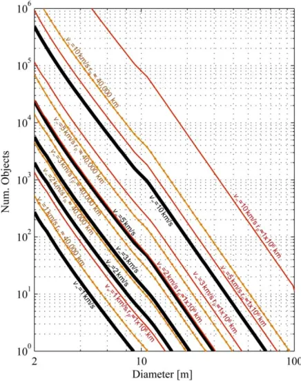
8], the most accessible objects, those requiring a lesser specific energy (i.e., energy per unit mass), are those with orbits such that they naturally intersect the orbit of the Earth or pass very close to it. Figure 3 shows the expected number of these objects for a set of different fly-by conditions. The fly-by or Earth approach conditions are defined for a set of different maximum hyperbolic excess velocities v∞ (ranging from 1
to 10 km/s) and maximum MOID distances. The solid lines, for example, have a maximum MOID distance fixed
tod⊕, whered⊕is the Earth impact distance, or
asymptotic distance for which the periapsis of the hyperbolic motion would be equal to the Earth radius r⊕:
2
2 1
d r
r v
µ⊕
⊕ ⊕
⊕ ∞
= +
⋅ , (5)
where µ⊕is the gravitational constant of the Earth. The two thinner lines have a maximum MOID distance equal to the geostationary ring, i.e., ~40,000 km (dot and solid line combination), or the sphere of influence of the Earth, i.e., ~1x10⁶ km (thin solid line).
Figure 3: Total expected number of objects with given encounter conditions. Solid lines represent available material with MOID smaller than d⊕. Dot & thin solid line represents objects with MOID at 40,000 km and, finally, thin solid line represent MOID at 1x10⁶km. Different relative velocity at encounter v∞ are given for each one of these three fixed MOID distances. The object estimation represents the average expected number of asteroids within ± 1 m of the size given by the abscissas axis.
[image:5.612.67.297.232.400.2] [image:5.612.321.539.257.533.2]that would eventually allow the asteroid to fly by the Earth by only slightly modifying its period with a small phasing manouvre. It is important to stress that the objects estimated in Figure 3 are not objects expected to impact the Earth in the near future, but only objects with a minimum orbital distance (MOID) small enough that they could flyby the Earth if they were artificially forced to meet the Earth at the point of minimum orbital distance.
The hyperbolic excess velocity v∞ parameter is
computed assuming a two-body patched conic approximation. At very low relative velocities, e.g., 1 - 2 km/s, the real trajectory may differ substantially to that of a hyperbola and three-body dynamics should be taken into account to understand the motion of these low-relative-velocity objects. Natural ballistic Earth capture or escape trajectories are indeed possible for objects with relative veloticies v∞ bellow 1 km/s (e.g.,[13]), as seen in a three-body dynamical analysis. Thus, objects moving towards the Earth at such a low relative velocities could become potential targets for ballistic Earth capture. As Figure 3 shows, there should be a non-negligible number of objects approaching the Earth with v∞ bellow 1 km/s. Most likely, no large object will be found fulfilling this low-velocity approach criterion, but a vast number of meter-sized objects should nevertheless be expected. Thus, these potential targets for ballistic capture should pose no impact risk to Earth [14], while may still render opportunities for technology demonstrator or science missions.
Current propulsion systems can be used to modify the linear momentum of spacecraft with masses of order 103 kg. Thus, envisaging the use of state-of-the-art propulsion systems altering the orbital motion of small asteroids (>>103 kg) implies a much lower acceleration than those achieved on spacecraft. It is because of this that the orbital insertion manoeuvre during Earth fly-by of such heavy objects is a critical manoeuvre. If the manoeuvre is not performed successfully, and the asteroid flies away from Earth, the following capture opportunity may occur many years later or never again. Moreover, the time that the asteroid spends under the gravitational influence of the Earth is limited and, thus, the required orbital manoeuvres must be performed in a relatively short time interval.
III. BALLISTIC CAPTURE
Ballistic capture trajectories with natural insertion into a bound Earth orbit must therefore be considered as a realistic means to provide capture opportunities for asteroid exploitation. An Earth ballistic capture exploits a natural low energy transfer to achieve a trajectory that switches from an initially Sun-centred to a final Earth-centred orbit [15]. In general, these types of natural Earth orbital insertions are only temporary, and, if no
manoeuvre is performed, the asteroid would eventually escape from the Earth’s gravitational influence. Nevertheless, the main advantage of envisaging ballistic capture as the entry channel of exploitable material is twofold: firstly, it allows an extended duration in the vicinity of the Earth which is advantageous when orbital manoeuvres are intended to be applied, and secondly, the Earth-centred orbit can be stabilized into a permanent Earth-bound orbit at a much lower cost than any other Earth encounter conditions.
Ballistic capture trajectories cannot be analysed using the classical patched-conic approximation and, at least, a restricted three-body model is required. The circular restricted three-body problem (CR3BP) is used here to characterise the general motion of asteroids under the influence of the Sun and the Earth. The dimensionless equations of motion in a rotating reference frame that describe the motion of an object in the CR3BP are:
2 U x y x ∂ − = ∂ 2 U y x y ∂ + = ∂
, (6)
U z z ∂ = ∂
where the non-dimensional potential function U is given by the expression:
(
)
(
2 2)
1 2
1 1
, , 2
U x y z x y µ µ
ρ ρ
−
= + + + . (7)
Here the reference frame is centred at the barycentre of the two major bodies and rotates with an angular velocity normalised to unity. The distance between the two gravitational bodies, Sun and Earth, is also normalised to one. The distances 1 and 2 are the distances from the particle, an asteroid in this case, to the primary mass (i.e., Sun) and secondary mass (i.e., Earth) respectively and is the standard mass parameter, which for the Sun-Earth system is 3.0032x10⁻⁶.
Eq.(6) has one integral of motion, the Jacobi integral:
(
)
2 2 2
1 2
1
2 2
v x y µ µ C
ρ ρ
−
= + + + − , (8)
where v2 is the velocity of the particle (i.e., asteroid) in the rotating frame and C is the Jacobi constant. This integral of motion is useful to define five distinctive motion regimes corresponding to values of C below or above the Jacobi constants corresponding to the five fixed equilibrium positions of Eq.(6) [16].
reference frame centred at the secondary mass, the Earth in this case, as:
(
)
(
)
(
)
2 2 2 2 22 2 2
2
2 2
1 2 1
1 2 2 1 2 x x y x v r
r r C
r µ µ µ µ ρ ρ = − + − − + + + + − + +
, (9)
where the vector 2
=
r
2xr
2yr
2z
is the asteroid position vector relative to Earth in the rotational reference frame.Here, an asteroid is said to be captured when it is inserted into an Earth bound orbit. Classical Keplerian elements can be used as osculating orbital elements, which define the instantaneous approximation of the motion of the object under the influence of Earth and Sun as a conic solution. Then, the boundary between an Earth bound and an escape orbit can be defined as an Earth-centred parabolic orbit. Thus, the velocity of a captured asteroid at the periapsis of its orbit needs to be smaller
than
v
p=
2
µ
⊕r
p , where µ⊕is the gravitational constant of the Earth and rp the periapsis distance. Note that vp is expressed in an inertial reference frame, while v, in Eq.(9), is expressed in a rotational frame. At periapsis distances rp at low-Earth orbit, however, angular velocity terms can be ignored. Using the non-dimensionalised vp in Eq.(9), and neglecting small terms, allows us to estimate the maximum Jacobi constant of the ballistically captured material:(
)
2(
)
2
2 2
1
1 2 2 2
1 th p a C r
µ
µ
µ
µ
ρ
µ
ρ
⊕ ⊕ − ≈ − + + − + , (10)
Eq.(10) estimates a Jacobi constant threshold Cth only marginally larger than that of the Jacobi constant of the Sun-Earth L4-L5 equilibrium points (C4-5). The value of
Cth defines therefore an asteroid moving in the motion regime where no prohibited zones can be described, and the asteroid can theoretically wander anywhere in the three-body system.
Since the parameter Cth is an integral of motion, and thus remains constant for the entire trajectory of the asteroid, generic threshold excess velocities v∞ at the Earth encounter can be extrapolated. By defining the
radius of the sphere of influence as rin=
(
m⊕ m)
2/ 5[17], where m⊕ is the mass of the Earth and m the mass of the Sun, which defines the distance from Earth at whichthe asteroids moves into the ‘bubble’ where Earth’s
gravitational influence dominates over the Sun’s, we can now use the constant Cth and Eq.(9) to define the
[image:7.612.316.542.312.462.2]threshold excess velocity v∞ of ballistically capturable objects.
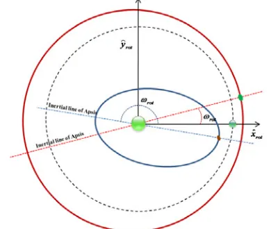
Figure 4: Earth relative position in polar coordinates.
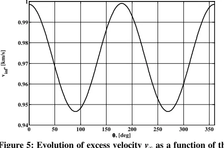
While at very close distances angular velocity and relative position terms can be ignored, at a distance rin from the Earth they need to be taken into account. Figure 4 shows the diagram of the polar coordinates used to describe the relative position and velocity of the incoming asteroid. The hyperbolic excess velocity is assumed here to follow a radial direction. Figure 5 shows the variation of excess velocity v∞ as a function of the polar angle . As shown in Figure 5 and as also stated in the previous section; ballistic captures of objects encountering the Earth with relative velocities close to 1 km/s are possible.
Figure 5: Evolution of excess velocity v∞ as a function of the
polar angle at a distance rin =
(
m⊕ m)
2/ 5 from Earth and Cth= 2.9999875750.While Cth can be used to estimate the maximum 3-body energy level of the ballistically capturable objects,
C2, or the Jacobi constant of a particle stationary at L2 equilibrium position [16], sets the minimum allowed energy for asteroid transitions from Sun to Earth centred orbits, for objects with semimajor axis larger than 1 AU. Similarly, then, generic excess velocity v∞ of objects approaching the Earth with Jacobi constant C2 can be estimated. The latter indicates that at the lower threshold for ballistic capture objects could approach the Earth at excess velocities of approximately 400 m/s and could be inserted into highly elliptical orbits with eccentricities slightly lower than 0.987.
From the preceding analysis, it can then be assumed that all asteroids moving with Jacobi constant smaller than C2 but larger than Cth are potential targets to be ballistically captured at Earth; at least, from an energy
0 50 100 150 200 250 300 350
0.94 0.95 0.96 0.97 0.98 0.99 1
θ, [deg]
standpoint. Note that, since the Jacobi constant is equal to minus twice the energy of the particle, the latter is equivalent to energy above C2 but bellow Cth. Similarly, asteroids with semimajor axis lower than 1 AU could be ballistically captured if moving with Jacobi constant
C1>C> Cth, where C1 is the Jacobi constant of a particle stationary at L1 equilibrium position. It is important to highlight that an asteroid moving with C2,1>C>Cth can as easily escape the Earth system as it was captured into it, unless stabilised into an energy bellow C1 while being in an Earth bound orbit.
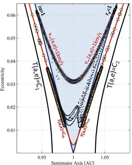
The evolution of the orbits that evolve into parabolic trajectories at the Earth periapsis, defined here as the threshold orbit between Earth escape and capture trajectories, can be studied by propagating backwards in time a set of final periapsis conditions.
III.II Incoming ballistic capturable material
Figure 6 shows the schematic of this backward propagation, while the summary of the results on evolution of the Sun-centred phase of a set of planar trajectories (inclination i=0o) is presented in Figure 7.
Figure 6: Schematics of the evolution of Sun-centred trajectories previous to a parabolic fly-by of the Earth.
The analysed set of final periapsis conditions has been constructed with 720 different final planar parabolic conditions at a perigee altitude of 200 km. Each initial condition in the set is propagated backwards using a planar CR3BP dynamics until the trajectory reaches the furthest distance from the Earth, thus when the trajectory is approximately at 2 AU distance from the Earth (see the schematics in Figure 6). All the initial conditions were set by homogenously distributing the parabolic velocity at the periapsis vparound the 2 range of the polar angle and both counter-clock and clock-wise directions for the vp were used (see Figure 6). Hence, two different initial conditions are analysed at each one degree step of the angle around the Earth. Instead of showing the full time evolution of the osculating semimajor axis and eccentricity, (a(t),e(t)), Figure 7 shows only a discrete set for the sake of clarity. The first value plotted, using a circle mark for each final condition, is at the t0 were the orbit meets plane x=0. Secondly, a set (a(tn),e(tn)) is
plotted for each n perihelion passage (i.e., true anomaly is equal to zero) and are marked with a small dot. The final value of (a(t),e(t)) corresponds to the time when the trajectory intersects the sphere of influence rin of the Earth and is marked with a cross.
Figure 7: Summary of the evolution of Sun-centred trajectories previous to a parabolic fly-by of the Earth. Shaded area highlights the Earth-crossing region.
[image:8.612.320.534.162.429.2] [image:8.612.67.291.344.430.2]The Tisserand parameter T,
(
2)
( )
1
2 1 cos
T a e i
a
=+ − , (11)
is a good approximation of the Jacobi constant for cases where the asteroid is far from the gravitational influence of the Earth [17], and this can indeed be seen in Figure 7. All the initial sets of conditions depart from very close to
the line defined by
(
(
)
)
1 2
1 2
2 1 th
a− + a −e =C . Half of the
initial conditions lie in a line slightly above T(a,e)=Cth, while the other half lie slightly bellow, this is simply due to the fact that when computing the constant Cth we have previously ignored the angular velocity terms. Now these have become apparent when counter clock-wise vp result in a slightly higher energy than a clock-wise vp.
Figure 8: Evolution of a set of unstable invariant manifolds of Lyapunov orbits with energies equal to: (C2+C3)/2, C3,
C4 and Cth. A) The manifolds were propagated
backwards until reaching the furthest distance from Earth (~2 AU), where semimajor axis and eccentricity were computed. B) All osculating elements of these manifolds spread on top of isolines of constant Tisserand parameter, or Jacobi constant, within the energy limits
C2 >C>Cth.
Finally, Figure 7 also shows the T(a,e)=C1 and
T(a,e)=C2 lines which, together with T(a,e)=Cth, limit the planar 3BP energy band where asteroid resources could be found with energies such that ballistic capture transfers are possible. This type of graph has been named elsewhere as a Tisserand-Poincaré graph [18], and it is believed to provide graphical hints that ballistic transfers between different sets of {a,e} under the same three-body energy (i.e., Jacobi constant) are possible. Indeed, one can search for Lyapunov orbits of different energy levels and analyse its unstable invariant manifold and see that all of them migrate from within these {a,e} regions. The set of unstable manifolds analysed in Figure 8, for example, reveal some clear hints on the existence of low-energy transport channels located within the energy limits C2 >C>Cth.
While in the previous section only the planar case was studied, the use of the Tisserand parameter T(a,e,i), Eq.(11), as an approximation of the Jacobi constant can be readily used to delimit the 3-dimensional Keplerian {a,e,i}-subspace from which asteroidal material could theoretically be ballistically captured.
III.III Total amount of capturable material
[image:9.612.69.282.290.544.2]Figure 10 shows the four planes delimiting the {a,e,i}-region with Jacobi constant C2>C>Cth if the semimajor axis is larger than 1 AU or C1>C>Cth for semimajor axis smaller than 1 AU.
Figure 10 shows two planes, so close together that they almost appear to be a single plane, curving within the Amor and Interior-Earth orbital region. Only a zoom into the region close to 1 AU shows the separation between these two planes. The question that may arise now is how many objects can be found on such a narrow band of energies. A quick search through the existing 8036 near-Earth objects (as on 14th July 2011) returns already 10 objects within this narrow band of Jacobi constants. These objects range in semimajor axis from 1.11 to 2.46 AU and in absolute magnitude from 17.1 to 24.96. The latter should correspond to objects ranging from half-kilometre to meter size respectively.
On the other hand, integrating the NEO distribution (a,e,i) within the Keplerian volume defined by these constant Jacobi energy band, the total fraction of asteroid population within these bands is 8.6x10⁻⁴. This is actually a large fraction of the NEO population, considering the narrowness of the integrated volume. Assuming then an estimate of the total NEO mass of order 4.4x10¹⁶kg [8], the total reservoir of material with Jacobi constant within
C2,1>C> Cth results 3.8x10 13
distribution of asteroids with Jacobi constant within
[image:10.612.68.291.138.340.2]C2,1>C>Cth is approximately 700 m diameter, while about 10 objects larger than 250 m diameter should also be expected.
Figure 9: Exploitable mass and probability density within {a,e,i}-space for low-energy transfers. The mass on the left y axis represents the total exploitable mass within a ±0.0025 range.
These hypothetical objects, however, may exist with orbital configurations extending far from the orbital neighbourhood of Earth (i.e., a≈1 AU and e≈0). Indeed,
this is shown in Figure 9. The figure reveals that the highest asteroid probability density or highest mass density within {a,e,i}-space for low-energy transfers occurs at 2.16 AU. Thus, we shall expect that the hypothesized large exploitable object may exist with semimajor axis extending far from 1 AU. Moving large objects from 2 AU to the Earth’s orbital neighbourhood may however take an unrealistic length of time by both means; natural (i.e., judicious use gravitational perturbations) or artificial transport (i.e., use of propulsion systems). We shall discuss this issue in the following section.
Figure 10: Planes of constant Jacobi integral (i.e., C1, C2 andCth ) and planes delimiting the regions with the three
[image:10.612.66.518.391.630.2]The previous section has shown that an important quantity of asteroid resources may be found in orbital regions where material could be retrieved by means of low-energy, quasi-ballistic, transfers.
IV.ASTEROID TRANSPORT TO EARTH ORBITAL NEIGHBOURHOOD
Figure 9, however, showed that the largest objects, and largest amount of resources, are likely to be found far from the Earth’s orbital neighbourhood. The scope of this section is then to investigate the feasibility of accessing these asteroid resources by means of low-energy transfers by considering now also estimates of their transfer times.
One possible alternative to study the transport of material by means of low-energy transfers is analysing a densely populated grid of unstable invariant manifolds of the two Sun-Earth collinear librations points. These asymptotic trajectories draw the transportation patterns that naturally provide transit trajectories between different orbit regimes [19, 20], what has become know as interplanetary superhighways [21]. Unfortunately, this approach would require a prohibitive computational power if one requires investigating low-energy transfer trajectories extending far from the Earth’s orbital neighbourhood. An alternative approach is to study multiple resonant gravity assists that would allow asteroids to move down the narrow energy band plotted in Figure 10 and fall into regions more densely populated with manifold “tubes”, as in Figure 8.
The latter approach can be analysed by means of a
Keplerian Map. The so-called Keplerian Maps were introduced by Ross and Scheeres [22], and provide a simple analytical approximation of the gravitational perturbation due to the secondary body on a planar CR3BP that allows us to efficiently estimate the maximum change of semimajor axis as a function of time that can be achieved by means of low-energy transfers. The Keplerian Map approach captures the dynamics of the full set of equations of motion, while simplifying enormously their computation [22].
A map is generally referred to as a function that associates consecutive sets of elements. In this case, the sets of elements are osculating Keplerian elements of the orbit at each apsis passage (see Figure 11). This update map of the apsis conditions is especially useful to understand the perturbations experienced by an object orbiting a primary object, e.g., the Sun, whose orbit is altered by a close approach to a secondary body, e.g., the Earth. The map integrates the first-order perturbation caused by the gravitational force of the secondary body and computes the change yielded on the set of Keplerian elements over the nominal orbit. Hence, the Keplerian map is only valid for cases for which the trajectory only grazes the sphere of influence of the secondary, or in
other words, it reproduces a gravity assist that occurs outside the sphere of influence of the secondary body. Nevertheless, the accuracy of the approximation has been proven both visually through comparison with a numerically integrated Poincaré map [22] and numerically by means of comparing the numerically integrated osculating elements [23].
The map is an expressed as a two-dimensional update such as:
(
)
(
)
3 2
1 1
1
2 2
, ,
n n n
n n n n
K
K K f K J
ω ω π
µ ω −
+ +
+
− −
=
+
(12)
where K is the two-body energy, i.e., K=-1/2a, is the rotating argument of the periapsis, J is the Jacobi constant and f( ,K,J) is the energy kick function, which estimates the two-body energy change at each encounter. Figure 11 shows a schematic of the system of interest here, which is that of an asteroid that does not cross the orbit of the Earth but is nevertheless perturbed by its gravity influence. This tool can then be used to analyse the motion of both Amor and Interior-Earth-Orbit asteroids (IEO), which, as shown by Figure 10, are the asteroid types that may be found with energies between C2>C>Cth or C1>C> Cth, respectively. Note that Eq.(12) refers to a planar system, thus this analysis is valid only for objects with very low inclination.
Figure 11: Keplerian map reference diagram. Two type of asteroids, Amor and Interior-Earth-Orbit asteroids (IEO), perturbed by the Earth gravity when their orbital paths pass close to Earth.
It is also important to note from Eq.(12) that the rotating argument at the periapsis passage changes only as a direct consequence of the ratio between the orbital periods of the Earth and the asteroid, thus, when the asteroid has completed one orbit, t=2 (a/GMSun)3/2, the Earth has completed an angular motion of
[image:11.612.333.528.403.568.2]as typically for the CR3BP, becomes =-2 a3/2. The Earth perturbation is then only taken into account by means of the semi-analytical expression referred as the energy kick function f( ,K,J), see appendices or for full details refer to its derivation in [22]. As seen in Figure 12, the energy kick function estimates the change in the two-body energy (i.e., semimajor axis a) by computing the perturbation caused by the Earth, in this case. In order to reduce the semimajor axis of an Amor type of asteroid the object should encounter the Earth with a rotating argument of periapsis slightly larger than zero, while to increase the semimajor axis of IEOs the asteroid should encounter the Earth with a slightly lower than .
Figure 12: Examples of energy kicks for a periapsis perturbation (i.e., periapsis kick function) and apoapsis perturbation (i.e., apoapsis kick).
Let us assume, for example, an asteroid with a semimajor axis of 2.25 AU (median of the probability density shown in Figure 9) and Jacobi constant Cth. The maximum change of semimajor axis is achieved for an argument equal to 4 degrees, which yields a negative change of 0.0018 AU. The energy kick function f( ,K,J) depends also on the Jacobi constant, but differences are small enough to ignore them (3x10⁻⁵ AU smaller for an asteroid with a Jacobi constant C2) and assume thereafter a Jacobi constant Cth unless stated otherwise. This optimal kick a is achieved during one single complete orbital revolution of the asteroid. A comparable change of semimajor axis could be achieved on a 10 m object with a continuous thrust of 100 mN. Here, 100 mN of thrust is chosen as a common low-thrust system for an interplanetary mission [24]. The gravitational kick provided by the Earth affects equally all asteroid sizes however. This clearly highlights the potential of judicious use of gravitational perturbations.
Unfortunately, this gravitational kick used as an example could not possibly be applied to the same asteroid at each orbit. Once the asteroid has been perturbed by an encounter occurring with a rotational argument of 4 degrees, the same asteroid may require
to complete many orbits before the proper geometry repeats, and indeed, it is quite possible that the asteroid will encounter the Earth with a geometry such that an opposite perturbation occurs and any gain is lost. Note, from Figure 12, that outside a very narrow region on the argument the perturbation produced by the Earth can be neglected, thus the asteroid can be assumed to be “kicked” only if encountering the Earth within this narrow -band.
Since multiple random perturbations will tend to cancel out, in order for an asteroid to experience large energy changes due to multiple accumulative perturbations the asteroid requires using resonant encounters with Earth. This will allow the asteroid to meet the Earth with the proper configuration at each consecutive encounter. Figure 13 shows all the possible resonances with Earth of the 2.25 AU asteroid. Thus, for example, resonance 62:209 provides a -0.0018 AU kick and allows the asteroid to encounter the Earth with the same geometry after 62 full asteroid orbits or 209 years. Note that the resonance 35:118 yields a lower -0.0016 AU change, but encountering the Earth again after 118 years, making it a more efficient resonance to use than 62:209.
The resonances are computed here by finding the semimajor axis a, within the attainable set, that yields a change of asteroid argument at the n revolution equal to
zero (mod 2 ). Perturbations are assumed to occur only
[image:12.612.68.290.239.390.2]Figure 13: Possible resonances with Earth of an asteroid with a semimajor axis of 2.25 AU. Resonances are expressed through two numbers: the number on the left refers to the number of asteroid orbits, while the number on the right is the number of Earth orbits.
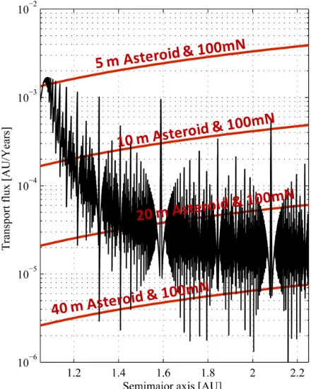
Hence the set of possible resonances at each possible asteroid semimajor axis provide the hints to understand the feasibly attainable transport fluxes for asteroids being transported by means of judicious use of the Earth’s gravitational perturbation. Figure 14 shows the transport flux, i.e., a/t where a is the change of semimajor axis achieved to enter a resonance and t is the time to the following kick. Only the optimal resonances, thus the resonances that yield the largest a/t, are accounted to plot Figure 14.
The rapid fluctuations of the transport flux as a function of a are due to the fact that specific resonances are reachable only from very close to the semimajor axis
a that defines the resonance. Thus, for example, with a
equal to 1.5874 AU, we enter a 1:2 resonance that greatly increases the value of the transport flux a/t simply because the following encounter, and kick, occurs only 2 years later. Only 0.002 AU away from 1.5874 AU, the 1:2 resonance is not reachable and any possible encounter take about 100 years to repeat. This indicates that the time
[image:13.612.317.537.87.362.2]t to the following encounter is the main driver affecting the value of transport flux, since in general the maximum kick is relatively unchanged for similar values of semimajor axis. Thus, as expected, the capability to produce large changes in semimajor axis is reduced once the timing for the following correct phasing is taken into account. Nevertheless, Figure 14 still shows that taking advantage of the Earth’s gravitational perturbation, even if weak, allows changing the orbit of large objects much more rapidly that what could be achieved with standard low-thrust propulsion capabilities.
Figure 14: Estimates on asteroid transport flux as a function of semimajor axis.
Following to Figure 14, we can now estimate the time that would take to transport an asteroid from an initial semimajor axis a0 to a final af equal to 1, where the asteroid could finally be inserted into an Earth centred orbit. With this purpose, the transport flux f(a) is integrated between a given a0 and 1 AU as:
( )
0
0
1 1
1
AU a AU
a
t da
f a
→
∆ =
∫
, (13)where ∆t is then the expected time to transfer from a0 to1 AU. The transport flux f(a) has been computed using a grid with a step size of 1x10⁻⁴ AU. Thus, the integration in Eq.(13), and since most of the resonances provide
a>1x10⁻⁴ AU, returns a
0 1
a AU t →
∆ that is averaged by the
[image:13.612.67.289.88.229.2]Figure 15: Expected transport times to reach a semimajor axis equal to that of Earth.
Unfortunately, Figure 15 demonstrates that the use of low-energy transfers can be extended only to the closest neighbourhood to Earth. The time required to capture at Earth objects with initial semimajor axis larger than 1.6 AU, for example, would already take more than a thousand years, which is clearly too long to be of any practical interest. We can however impose a maximum transfer time of 100 years as of practical interest. The results plotted in Figure 15 delimit the feasible boundaries for a 100 years capture of material from 0.9 AU to 1.135 AU. The total NEA fraction within these limits and with Jacobi constants within C2(or 1)>C> Cth is 8.4x10
-7
, which is equivalent to an approximate value of 3.7x10¹⁰kg of asteroid material. In terms of objects, one can compute the median size and the 90% confidence region of the largest asteroid as described in [8]. The median largest asteroid to be expected with these orbital characteristics is around 30 meters diameter, while the Poison 90% accumulative probability is achieved between 20 and 50 meters diameter. Also, statistically, an average of 40 objects of 10 meters should be found within the Keplerian space from where ballistic capture should be feasible in less than a 100 years. Note this transfer time estimate is only the maximum allowed transfer time to delimit the feasible capture region (from 0.9AU to 1.135 AU). Individual objects will require transfer time from 0 to 100 years, and not necessarily the upper boundary.
This paper has discussed the possibility of capturing near Earth objects into bound Earth orbits. The ‘new-moon’ concept for asteroid exploitation has been suggested a number of times on futuristic views of a space industrialization. This paper however has attempted to place realistic bounds on the concept by investigating the availability of asteroids on orbits from which retrieval is technically feasible. It has been shown that gravitational perturbations must play a paramount role on the dynamics of any asteroid transfer to Earth.
V. CONCLUSIONS
The paper has shown that a fraction of order 10-3 of the NEA population lies on Keplerian regions where low-energy transfers to Earth with ballistic capture opportunities exist. Assuming a power law distribution for the population of asteroids, this fraction indicates that several objects larger than 500 m should exist with the potential of being captured at Earth with the expenditure of a minimal amount of energy. Despite the latter result, the paper has also shown that any likely large asteroids would require an impractically large transfer time or the use of propulsion systems orders of magnitude more powerful and efficient than current technologies allow.
Nevertheless, it has also been shown that that it is still feasible to find objects close enough to the Earth’s neighbourhood so that their low-energy transfers can be completed in less than 100 years (this being only an upper bound). The largest of these should be on the order of 30 meters, while an average of 40 objects should be found with diameters larger or equal to 10 meters. These small objects may seem uninteresting because of their small size, but they can still deliver important quantities of specific materials, without posing any impact risk to the Earth. Hence they probably are candidates for technology demonstrator missions.
We thank William Bottke for kindly providing us with the NEA distribution data. We also thank the Faculty of Engineering High Performance Computer facility, University of Strathclyde. The work reported was supported by European Research Council grant 227571 (VISIONSPACE).
[image:14.612.77.286.88.351.2]APENDICES
The energy kick function f( ,K,J) takes two forms. A periapsis version:
Energy Kick Function
(
)
(
)
( )
3 2 0 1 , ,sin 2 sin cos( )
p
f K J
p
r
t d t d
r
π π
π
ω
ω ν ν ω ν ν
− = − × + − − −
∫
∫
(14)where p is the semilatus rectum, r the distance from the asteroid to the Sun (r=p
(
1+ecos( )ν
)
), r2 the distance from the asteroid to Earth(r2 = 1+ −r3 2 cos(r
ω ν
+ −t)), ν is the true anomalyof the asteroid orbit, and finally, 3/ 2
( )
t=a M ν , where M
is the mean anomaly. While fp applies to asteroids with a semimajor axis a larger than 1 AU, an apoapsis version applies to a<1AU:
(
)
2 3(
)
2 0 1
, , 1 sin
a
r
f K J t d
r p
π
ω
= − +ω ν
+ −ν
∫
(15)
Note that the K defines the semimajor axis, while J defines the eccentricity by means of Eq.(11) in the planar case.
[1] Tsiolkovsky, K. E., “The Exploration of Cosmic
Space by Means of Reaction Devices,” Scientific Review, No. 5, 1903.
REFERENCES
[2] Mckay, M. F., McKay, D. S. and Duke, M. B.,
“Space Resources,” Lyndon B. Johnson Space Center, 1992.
[3] Cole, D. M. and Cox, D. W., Islands in Space:
The Challenge of Planetoids., Chilton Books, Philadelphia, 1964, p.^pp. 276.
[4] O'Leary, B., “Mining the Apollo and Amor
Asteroids,” Science, Vol. 197, No. 4301, 1977, pp. 363-366 doi: 10.1126/science.197.4301.363-a
[5] Lewis, J. S., “Platinum Apples of the Asteroids,”
Nature, Vol. 372, 1994, pp. 499 - 500. doi: 10.1038/372499a0
[6] Alvarez, L. W., Alvarez, W., Asaro, F. and
Michel, H. V., “Extraterrestrial Cause for the Cretaceous-Tertiary Extinction,” Science, Vol. 208, No. 4448, 1980, pp. 1095-1108. doi: 10.1126/science.208.4448.1095
[7] Morbidelli, A., Bottke, W. F., Froeschlé, C. and Michel, P., Asteroids Iii, University of Arizona Press, Tucson, 2002, pp. 409-422.
[8] Sanchez, J. P. and McInnes, C. R., “Asteroid
Resource Map for near-Earth Space,” Journal of Spacecraft and Rockets, Vol. 48, No. 1, 2011, pp. 153-165. doi: 10.2514/1.49851
[9] Bottke, W. F., Morbidelli, A., Jedicke, R., Petit, J.-M., Levison, H. F., Michel, P. and Metcalfe, T. S., “Debiased Orbital and Absolute Magnitude Distribution of the near-Earth Objects,” Icarus, Vol. 156, No. 2, 2002, pp. 399-433. doi: 10.1006/icar.2001.6788
[10] Harris, A. W., “An Update of the Population of
Neas and Impact Risk,” Bulletin of the American Astronomical Society, Vol. 39, 2007, p. 511. doi: 2007DPS....39.5001H
[11] Stokes, G. H., Yeomans, D. K., Bottke, W. F.,
Chesley, S. R., Evans, J. B., Gold, R. E., Harris, A. W., Jewitt, D., Kelso, T. S., McMillan, R. S., Spahr, T. B. and Worden, P., “Study to Determine the Feasibility of Extending the Search for near-Earth Objects to Smaller Limiting Diameters,” NASA, 2003.
[12] Harris, A. W., “What Spaceguard Did,” nature,
Vol. 453, 2008, pp. 1178-1179. doi:
10.1038/4531178a
[13] Kemble, S., “Interplanetary Missions Utilising
Capture and Escape through the Lagrange Points,” Proceedings of the 54th International Astronautical Congress, edited by I.A. Federation, Vol. IAC-03-A.1.01, Bremen, Germany, 2003.
[14] Hills, J. G. and Goda, M. P., “The Fragmentation
of Small Asteroids in the Atmosphere,” The
Astronomical Journal, Vol. 105, No. 3, 1993, pp. 1114-1144. doi: 10.1086/116499
[15] Marsden, J. E. and Ross, S. D., “New Methods in Celestial Mechanics and Mission Design,”
Bulletin of the American Mathematical Society, Vol. 43, No. 1, 2005, pp. 43-73.
[16] Schaub, H. and Junkins, J. L., Analytical
Mechanics of Space Systems, Aiaa Educational Series, American Institute of Aeronautics and Astronautics, 2003.
[17] Battin, R. H., Introduction to the Mathematics and Methods of Astrodynamics Aiaa Education Series, American Institute of Aeronautics and Astronautics, Reston, Virginia, 1999.
[18] Campagnola, S. and Russell, R. P., “Endgame
Problem Part 2: Multibody Technique and the
Tisserand-Poincare Graph ” Journal of
[19] Gómez, G., Koon, W. S., Lo, M. W., Marsden, J. E., Masdemont, J. and Ross, S. D., “Invariant Manifolds, the Spatial Three-Body Problem and
Space Mission Design,” Proceedings of the
AIAA/AAS Astrodynamics Specialist Meeting, Quebec City, Quebec, Canada, 2001.
[20] Ross, S. D., “The Interplanetary Transport
Network,” American Scientist, Vol. 94, No. 3, 2006, p. 230. doi: 10.1511/2006.3.230
[21] Lo, M. W., “The Interplanetary Superhighway
and the Origins Program,”
IEEEAerospaceConference, Big Sky, MT, USA, 2002.
[22] Ross, S. D. and Scheeres, D. J., “Multiple
Gravity Assists, Capture, and Escape in the
Restricted Three-Body Problem,” SIAM J.
Applied Dynamical Systems, Vol. 6, No. 3, 2007, pp. 576-596. doi: 10.1137/060663374
[23] Lantoine, G., Russell, R. P. and Campagnola, S.,
“Optimization of Low-Energy Resonant
Hopping Transfers between Planetary Moons,”
Acta Astronautica, Vol. 68, No. 7-8, 2011, pp. 1361-1378 doi: 10.1016/j.actaastro.2010.09.021
[24] Rayman, M. D., Fraschetti, T. C., Raymond, C.
![Figure 1: Theoretical Bottke et al. [9] NEO distribution. The figure shows the integrated projections of the function �(a,e,i) and a set of grid points coloured and sized linearly with the values of the NEO density](https://thumb-us.123doks.com/thumbv2/123dok_us/1687528.122132/4.612.105.488.91.308/figure-theoretical-distribution-integrated-projections-function-coloured-linearly.webp)