Pond IDE: Machine level program development environment and register transfer level simulator for a massively parallel computer architecture

(1)

Theses Thesis/Dissertation Collections

2010

Pond IDE: Machine level program development

environment and register transfer level simulator for

a massively parallel computer architecture

Jesse Muszynski

Follow this and additional works at:http://scholarworks.rit.edu/theses

This Thesis is brought to you for free and open access by the Thesis/Dissertation Collections at RIT Scholar Works. It has been accepted for inclusion in Theses by an authorized administrator of RIT Scholar Works. For more information, please [email protected].

Recommended Citation

(2)

Massively Parallel Computer Architecture

by

Jesse J. Muszynski

A Thesis Submitted in

Partial Fulfillment of the

Requirements for the Degree of MASTER OFSCIENCE

in

Electrical Engineering

Approved by:

Dr. Dorin Patru, Assistant Professor

Thesis Advisor, Department of Electrical and Microelectronic Engineering

Dr. Eric Peskin, Assistant Professor

Committee Member, Department of Electrical and Microelectronic Engineering

Dr. Daniel B. Phillips, Associate Professor

Committee Member, Department of Electrical and Microelectronic Engineering

Dr. Sohail A. Dianat, Professor

Department Head, Department of Electrical and Microelectronic Engineering

DEPARTMENT OFELECTRICAL ANDMICROELECTRONICENGINEERING

KATEGLEASON COLLEGE OF ENGINEERING

ROCHESTERINSTITUTE OF TECHNOLOGY

ROCHESTER, NEW YORK

(3)

Rochester Institute of Technology

Kate Gleason College of Engineering

Title:

Pond IDE: Machine Level Program Development Environment and

Register Transfer Level Simulator for a Massively Parallel Computer

Architecture

I, Jesse J. Muszynski, hereby grant permission to the Wallace Memorial Library to reproduce my thesis in whole or part.

Jesse J. Muszynski

(4)

c

Copyright 2010 by Jesse J. Muszynski

(5)

Dedication

(6)

Acknowledgments

I would like to acknowledge my advisor, Dr. Patru for his contributions to this work and my committee members for their guidance and feedback in the preparation of this

document. Additionally I would like to acknowledge Trevor West, my friend and colleague, for his help consulting me on the proper development of the Computer Science

(7)

Abstract

Pond IDE: Machine Level Program Development Environment and Register

Transfer Level Simulator for a Massively Parallel Computer Architecture

Jesse J. Muszynski

Supervising Professor: Dr. Dorin Patru

As computing architectures are being implemented in late and post silicon technologies, fault tolerance and concurrent operation are becoming increasingly important. It is already common knowledge that manufacturers are putting two, four or even more cores on a sin-gle silicon die to improve computing performance. The proposed architecture far exceeds

this number by grouping thousands or even millions of simplereduced instruction set

com-puting (RISC) processors, each of which is capable of a single operation at a time, and to communicate with its eight nearest neighbors. In this architecture, if a single core or cluster of cores have defects at the time of manufacture, or later in the life of the system, it is possible to test and disable them as necessary.

A fine-grained architecture of this kind calls for a parallel programming style. One approach to this problem is the use of a parallelizing compiler. Another approach may be

to use one of the severalapplication programming interfaces(APIs) available for standard

text based programming languages, with some built-in features for parallel programming. This work has generated a solution for creating machine level parallel programs for the massively parallel computer architecture described above using text and graphical means.

To support this programming method, an integrated development environment (IDE) and

a zero communication latency, register transfer level (RTL) simulator have been

(8)

List of Tables

2.1 Information stored by one atomic processor, and its significance. Storage

requirements, in bits, for64K and1T seas of atomic processors. . . 9

2.2 The reduced instruction set. To meet the self-imposed requirement that

each atomic processor has to be a low complexity, processing element, we have included in the instruction set only fundamental arithmetic, logic, and control flow instructions. . . 10

2.3 Communications handshake codes. . . 13

2.4 Message routing scheme used during a global or entity casts. . . 15

2.5 Message formats. The numbers of bits in the shaded boxes change with the

size of the sea of atomic processors and/or size of operands. The message codes are described in Table 2.6. ID = Identification number; S = Source; D = Destination; I = Intermediate. . . 18

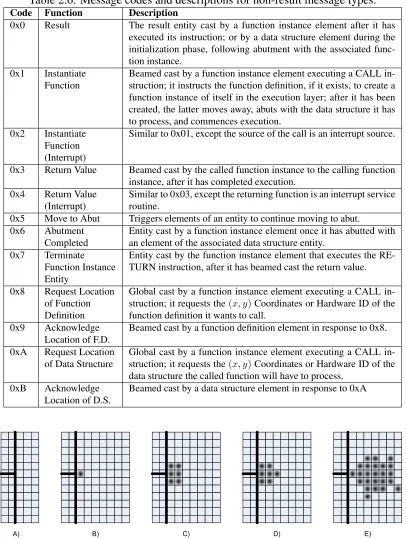
2.6 Message codes and descriptions for non-result message types. . . 20

(12)

List of Figures

2.1 The sea of atomic processors. Each atomic processor can communicate

with its eight adjacent neighbors. The input / output ports, illustrated in

bold lines, can be located at the periphery, or can penetrate the sea. . . 5

2.2 A snapshot of the sea of atomic processors. Programs are broken down into

functions. A function copy is stored in afunction definitionentity. When a

function is called, the function definition creates a copy, called afunction

instance. This moves away and abuts with the data structureentity it has

to process. . . 5

2.3 The communications hardware is divided into a send and receive layer.

Each layer uses a set of 8 handshake buffers and one message buffer. This allows full-duplex message passage. . . 12

2.4 A complete communications cycle. Atomic processor xis transmitting a

message to its neighbor, atomic processory. . . 14

2.5 Routing and propagation of a beamed, entity, and global cast messages. In

a beamed cast, the maximum number of atomic processors the message has

to pass through is equal tomax{|xs−xr|,|ys−yr|}, where the sender is

at(xs, ys)and the receiver is at (xr, yr). In an entity cast the propagation

stops at the edge of the entity. . . 16

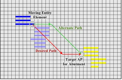
2.6 A moving entity is forced to move around another entity. Elements of the

moving entity move counterclockwise as many times as needed, and correct

their course as soon as possible afterwards. . . 17

2.7 An entity enters the sea of atomic processors, when viewed froma → f,

or exits the sea of atomic processors, when viewed fromf → a. Large

entities may be input or output via multiple ports and associated atomic

processors. . . 20

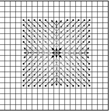
2.8 Routing and propagation of a global cast message. Using the scheme in

(13)

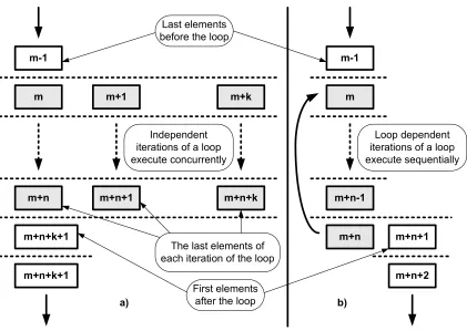
2.9 The execution of a loop without loop carried dependencies (a), and with loop carried dependencies (b). The gray shaded function instance elements are part of the loop iteration. . . 26

3.1 Text based code for the first four tokens of the 32-bit multiplier shown in

Figure 4.7. . . 29

3.2 IDE Property Grid . . . 32

3.3 Different tokens placed on the layout grid. . . 35

4.1 C code that calculates the first twelve elements of the Fibonacci series. . . . 40

4.2 Screen Capture of the Fibonacci Program showing the calculation of the

first twelve elements of the Fibonacci series. AP 10 returns the twelfth element to the calling function. Call out boxes have been added to show the values within each processor. . . 41

4.3 C Code that performs vector addition for two eight element vectors. . . 42

4.4 Screen Capture of the Vector Add Program showing two eight element

ar-rays of data elements, DEs 1 through 7 and 8 through 16, being added by APs 17 through 24. Call out boxes have been added indicating the operands, operation and output of each of the tokens. . . 43

4.5 C Code that performs integer multiplication using a left shift multiplication

algorithm. . . 44

4.6 Screen Capture of 32-bit Left Shift Integer Multiply Function Definition . . 45

4.7 Screen Capture of 32-bit Left Shift Multiply Simulation, multiplying

un-signed integers 5 and 10 to yield a result of 50. Call out boxes have been added to show the values within each processor. . . 46

4.8 C Code that unpacks the sign bit from the floating point number

represen-tation. . . 48

4.9 The sign bit of a floating point number is unpacked by simply masking the

MSB. Call out boxes have been added to show the operation performed by each processor. . . 49 4.10 C Code that unpacks the exponent portion of the floating point number

representation. . . 50 4.11 The exponent of a 32-bit floating point number is unpacked by masking off

(14)

4.12 C Code that unpacks the mantissa or significand portion of the floating point number representation. . . 52 4.13 The significand of a 32-bit floating point number is unpacked by masking

off the least significant 23 bits and adding a 1 in the 23rd bit position, where bit 0 is the LSB. Call out boxes have been added to show the operation performed by each processor. . . 53 4.14 C Code that packs a sign, exponent, and mantissa into the IEEE Floating

Point representation. . . 54

4.15 Packing operation for a 32-bit floating point number. The function defini-tion takes a sign, exponent and mantissa as inputs and outputs a floating point number. Call out boxes have been added to show the operation

per-formed by each processor. . . 55

4.16 C Code that performs a 24-bit fixed point multiplication using a right shift multiplication algorithm. . . 57 4.17 Right Shift Integer multiplier for 24 bit fixed point multiplication used in

floating point multiplication algorithm. Call out boxes have been added to show the operation performed by each processor. . . 58 4.18 C code that implements the top level floating point multiplication algorithm

by making calls to the previously mentioned C code. . . 60 4.19 Floating point multiply program with function calls to floating point

un-packing and un-packing operations and right shift fixed point (24bit integer) multiplier. Call out boxes have been added to show the operation performed by each processor. . . 61 4.20 C Code to perform division through iterative subtraction. . . 63 4.21 Example integer division algorithm [1]. . . 63

4.22 Screen Capture of sample division algorithm with Next Row to Execute

field and non-unique ID numbers indicated in call out boxes (Simulation

non-functional). . . 64

5.1 Export to Human Readable Code for the first four tokens of the 32-bit

mul-tiplier shown in Figure 4.7. . . 76

A.1 Example Project Properties Dialog from the 32-bit floating point number packing function. . . 92

(15)

A.3 Toolbar Buttons: A) Atomic Processor, B) Concurrent Array, C) Sequential Array, D) Data Element, E) Function Call, F) Design Mode, G) Simulation Mode. . . 95 A.4 IDE Property Grid . . . 99 A.5 A) The lines coming into AP1 are highlighted for easier reading, the line

exiting AP1 is in its normal unhighlighted state. B) The source token for AP2 has been deleted, a red stub remains. . . 100 A.6 Conditional Tokens A)Before Simulation tokens are yellow, B)During

Sim-ulation tokens change green or red based on if the condition is met. . . 101

A.7 Example of the 32-bit Left Shift Multiplier stopped at a breakpoint. . . 103

A.8 Example of the 32-bit Left Shift Multiplier stepped one step forward after

a breakpoint. . . 104

A.9 Example function call property grid for the Floating Point pack operation

(16)

Chapter 1

Background and Motivation

Parallelism and concurrency are inherent in many computational tasks. Techniques that

ex-ploit instruction and thread level parallelism in traditional von Neumann architectures have

been successfully applied in single processors, as described by Hennessey and Patterson

in [2]. During the past decade researchers and manufacturers have turned to multi-core

processors, which at the present time are limited to just a few cores [3–8]. Scaling up the

techniques used to exploit instruction and thread level parallelism in single core processors

to many core processors is challenging for both hardware and software designers [9–12].

As pointed out by Hennessy and Patterson in [2], multi-core processors are a

combi-nation of computer architecture and communications architecture. Computer networks on

a chip or cluster computing on a chip are adapting the vast knowledge base of designs

and architectures of macro computer networks to the micro scale, [13–26]. Marculescu

et al. in [27] classify outstanding research problems related to networks on chip into 15 categories. Predominant are problems related to communications infrastructure and

com-munications paradigms, as illustrated by [28–54]. Dongarra et al. explore the potential

symbiosis between networks on chip and multicore processors in [55].

Late and post silicon era integrated circuit fabrication technologies will continue to

(17)

number will not translate into an increase in performance unless new parallel and

concur-rent architectures are developed, as pointed out by Rabaey and Malik in [56], and Wen-mei

et al. in [57]. These new architectures will have to address reliability at the circuit and system levels because some components will experience premature, transient or permanent

failures, as highlighted by Austinet al.in [58]. Lei Zhanget al.address reliability and fault

tolerance in networks on chip in [59]. Power dissipation will have to be mitigated starting

at the system level. This is already being considered in multicore processors [60, 61], and

in networks on chip [62–67]. Nano architectures attempt to specifically address the

afore-mentioned challenges posed by late and post silicon technologies [68–76].

Taking into account the above considerations, a focus has been placed on exploring the

feasibility of a hardware design in massively parallel processing. The design itself consists

of an undetermined, but large number of simple, interconnected processing elements

re-ferred to as aseaof processors. Each element has the ability to communicate only with its

eight nearest neighbors through a dedicated message passing layer. Messages intended to

be passed a distance further than a nearest neighbor must propagate from processor to

pro-cessor using algorithms designed to optimize message passing using the shortest number

of hops to get to the intended recipients. While the design of the underling hardware is

im-portant and is discussed in Chapter 2, it is not the primary research focus. The architecture

organization and communication algorithms have been developed and described by Adam

Spirer in his thesis [1].

Accordingly, the current work focuses on the development of a machine level

program-ming environment, and register-transfer level simulator, for a massively parallel

architec-ture. The register-transfer level simulator assumes zero-latency communications. Initially,

the method of programming for the aforementioned architecture was performed in a C

like, text based format, but this quickly proved inadequate. The programming environment

(18)

program flow and register level information.

The organization of the architecture, including communications and operation, is

cov-ered in Chapter 2, followed by the description of the programming environment and

sim-ulation model of the architecture in Chapter 3. Experimental results are shown and

dis-cussed in Chapter 4, and development of the programming environment and simulator are

(19)

Chapter 2

Architecture Organization

An introduction to the architecture has been given in this chapter to provide the reader a

basis of what the machine level program development environment and register-transfer

level simulator aims to model. The chapters following this overview require this basis

for a solid understanding of the implemented model. The work introduced in this chapter

describing the development of the architecture is primarily the focus of Adam Spirer’s

thesis [1].

2.1

Architecture Overview

The proposed architecture is comprised of a sea of atomic processors, or atomic processing

elements, arranged in an orthogonal structure, as shown in Figure 2.1. All atomic

proces-sors are physically and functionally identical, but operationally independent. Each atomic

processor is a low-complexity processing element, capable of:

• Storing and executing one instruction, and storing its associated operands and result,

or

(20)

[image:20.612.105.512.325.620.2]

Input / Output Port AP (i,j) AP (i-1,j) AP (i-2,j) AP (i+1,j) AP (i+2,j) AP (i,j-1) AP (i-1,j-1) AP (i-2,j-1) AP (i-2,j-2) AP (i-1,j-2) AP (i,j-2) AP (i+1,j-2) AP (i+1,j-1) AP (i+2,j-1) AP (i+2,j-2) AP (i-2,j+1) AP (i-2,j+2) AP (i-1,j+1) AP (i-1,j+2) AP (i,j+1) AP (i,j+2) AP (i+1, j+1) AP (i+1, j+2) AP (i+2, j+1) AP (i+2, j+2)

Figure 2.1: The sea of atomic processors. Each atomic processor can communicate with its eight adjacent neighbors. The input / output ports, illustrated in bold lines, can be located at the periphery, or can penetrate the sea.

FI moving around dead APs DS moving between two other DSs

FD = Function Definition DS = Data Structure DS = Data Structure

FI = Function Instance Dead Atomic Processors

APs = Available Atomic Processors

FD = Function Definition

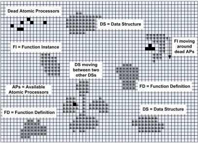
Figure 2.2: A snapshot of the sea of atomic processors. Programs are broken down into

functions. A function copy is stored in a function definition entity. When a function is

called, the function definition creates a copy, called a function instance. This moves away

(21)

In the sea of atomic processors, programs and data structures are organized as

morpho-logical entities, as shown in Figure 2.2. These can move, abut, and dissolve. As in the

C programming language, programs are broken down into functions. A function’s code is

stored in a function definition. When a function is called at runtime, the function

defini-tion creates an instance of the funcdefini-tion. The funcdefini-tion instance moves away, and eventually

abuts with the data structure that was passed to it by the calling function instance, before

commencing execution. Upon completing execution, the called function instance returns a

value or the result of processing in the form of a data structure.

Thus, in the sea of atomic processors as shown in Figure 2.2, we distinguish the

follow-ing morphological entities:

1. Function Definitions - FD. These are functions / programs not actively associated

with any data set or structure. An element of a function definition entity is an

in-struction word and its associated operand(s). In conventional architectures, these

entities are equivalent to copies of programs stored on hard disk or other high

ca-pacity storage media. These entities also include functions, which assist with input

/ output operations, and system level housekeeping. In conventional architectures,

these are equivalent to operating system functions.

2. Function Instances - FI. These are runtime instances of function definitions, which

can be or are already actively associated with a data set or structure. An element of

a function instance is an instruction word and its associated operand(s) and result. In

conventional architectures, these entities are equivalent to copies of programs loaded

at runtime into main memory.

3. Data Structures - DS. These are collections of associated data elements, which would

be processed by the same function instance. An element of a data structure is a data

(22)

complex as files on a hard disk or other high capacity storage media in conventional

architectures.

Not classified as morphological units,Dead Atomic Processorsare individual or groups

of atomic processors, which have been rendered not functional as a result of one or more

internal faults.

The architecture is inspired from the field of microbiology. The morphological entities

in the sea of atomic processors shown in Figure 2.2, move, change shape, and adapt like

microorganisms in a medium. The shape of an entity may change in the course of a

nor-mal move, a move around other entities or dead atomic processors, or to group together

associated elements.

Each atomic processor can store at the same time a function definition element, and a

function instance or data structure element. This breaks down the sea of atomic processors

into two functional layers: the definition layer, in which function definition elements are

stored, and the execution layer, in which function instance or data structure elements are

stored. In addition, in each layer the atomic processor stores configuration information

associated with each element.

The storage requirements for an atomic processor are summarized in Table 2.1. We

show for reference the size of each field in bits for a64K(216_{) and}₁_T ₍₂40_{) seas of atomic}

processors. The 64K sea of atomic processors is typical for a computer system used in

an embedded application, while the 1T is typical for a computer system used in desktop

applications. The morphological entity type indicates the momentary functional role of the

atomic processor. The hardware identification number contains thexandycoordinates of

the atomic processor, and does not change during the lifetime of the system. The entity

(23)

identification number identifies the element within the entity. The target entity

identifica-tion number and(x, y)coordinates are used during the move and abut processes, which are

described in Sections 2.4 and 2.6, respectively. The primary and secondary operand source

identification numbers indicate which element within the entity will provide the value of

these operands. Either of these can also be initialized. There can be up to 16 data types, of

which we currently encode: Boolean, character, character string, unsigned and signed

in-tegers of 16, 32, and 64 bits, single and double precision fixed and floating point numbers.

Theprevious execution order,execution order, execution countandexecution count iden-tification numberare used for execution flow control, as described in Sections 2.7 and 2.9. The operation code distinguishes between 256 different possible operations in the

instruc-tion set. Each instrucinstruc-tion can be executed uncondiinstruc-tionally or condiinstruc-tionally on the value of

four status bits. Their true and complemented values are stored in the execution conditions

field. The values of the status bits are produced by the element whose identification number

corresponds to the status bits source identification number.

2.2

Instruction Set

The reduced instruction set is listed in Table 2.2. To meet the self-imposed requirement that

each atomic processor has to be a low complexity processing element, we have included in

the instruction set only fundamental arithmetic, logic, and control flow instructions.

Com-plex or compound operations like multiplication or division are implemented as functions,

(24)

Table 2.1: Information stored by one atomic processor, and its significance. Storage

re-quirements, in bits, for64K and1T seas of atomic processors.

Name 64K 1T Value

METype 2 2 Morphological Entity Type (element)

0=Unoccupied; 1=FD ; 2=FI ; 3=DS Hardware ID 16 40 (x, y)coordinates of the atomic processor

Entity ID 16 40 Entity element identification number

Element ID 16 40 Entity element identification number

Target Entity ID 16 40 Target entity identification number used during the move and abut processes.

TargetEntityXYCoordinates 16 40 Target entity(x, y)coordinates used during the move and abut processes.

PrimaryOperandSourceID/ DataWordID

16 40 FD/FI:Primary operand source identification number; corresponds to an associated DS element data word ID SecondaryOperandSourceID 16 40 FD/FI:Secondary operand source identification num-ber; corresponds to an associated DS Entity ID or Ele-ment ID

PrimaryOperandType/ DataWordType (Execution)

4 4 FD/FI:Primary operand type; DS: Data word type SecondaryOperandType

(Execution)

4 4 FD/FI:Secondary operand type PrimaryOperandValue/

DataWordValue (Execution)

32 64 FD/FI:Primary operand value; DS: Data word value SecondaryOperandValue

(Execution)

32 64 FD/FI:Secondary operand value

PrevExecutionOrder 16 32 FD/FI: ExecutionOrder number, of element(s) that must execute before this element

ExecutionOrder 16 32 FD/FI:Element execution order number

ExecutionCount (Execution) 16 32 FI: How many times must this FI receive a result broadcast with a particular execution order number (from a previous instruction) before executing itself? ExecutionCountID 16 40 FI:Associated DS Element ID that also stores the

Ex-ecutionCountvalue

StatusBitsSourceID 16 40 FD/FI: Element ID whose execution result produces the status bits for this instruction (compared against Execution Conditions)

SourceStatusBitsValues 8 8 FD/FI: Status bits values received from Status-BitsSource

OperationCode 8 8 FD/FI:Instruction/operation code

ExecutionConditions 8 8 FD/FI:Status bits (C, N, V, Z, !C, !N, !V, !Z) required for execution of instruction

ResultValue (Execution) 32 64 FI:Result value of last execution ResultStatusBitsValues

(Execution)

8 8 FI:Result status bits of last execution

Cast Type 8 8

Total to Store: 386 754

To move FD/FI element: 274 538

(25)

Table 2.2: The reduced instruction set. To meet the self-imposed requirement that each atomic processor has to be a low complexity, processing element, we have included in the instruction set only fundamental arithmetic, logic, and control flow instructions.

Mnemonic Operation Code Operation

NOP 0x00 No operation.

ADDPS 0x01 Add primary and secondary operands.

ADDPC 0x02 Add carry and primary operand.

ADDPSC 0x03 Add primary operand, secondary operand, and carry.

SUBPS 0x04 Subtract secondary operand from primary operand.

SUBPC 0x05 Subtract carry from primary operand.

SUBPSC 0x06 Subtract secondary operand and carry from primary

operand.

INC 0x07 Increment primary operand.

DEC 0x08 Decrement primary operand.

INV 0x09 Bitwise inversion of primary operand.

AND 0x0A Bitwise AND of primary and secondary operands.

OR 0x0B Bitwise OR of primary and secondary operands.

XOR 0x0C Bitwise XOR of primary and secondary operands.

SETC 0x0D Explicitly set ‘carry’ flag.

SETZ 0x0E Explicitly set ‘zero’ flag.

SETN 0x0F Explicitly set ‘negative’ flag.

SETV 0x10 Explicitly set ‘overflow’ flag.

RSTC 0x11 Explicitly reset ‘carry’ flag.

RSTZ 0x12 Explicitly reset ‘zero’ flag.

RSTN 0x13 Explicitly reset ‘negative’ flag.

RSTV 0x14 Explicitly reset ‘overflow’ flag.

SHL 0x15 Shift left primary operand, pad with zeros.

SHR 0x16 Shift right primary operand, pad with MSB.

SHLC 0x17 Shift left primary operand through carry, pad with zeros. SHRC 0x18 Shift right primary operand through carry, pad with MSB. CALL 0x19 Function call instruction; requests the function defini-tion whose identificadefini-tion number is stored in the primary operand value to create an instance; the created function instance will process the data structure whose identifica-tion number is stored in the secondary operand value; the execution of this instruction completes when it receives a RETURN result from the called function instance. RETURN 0x1A Function return instruction; broadcasts return value of

(26)

2.3

Communications

Communications in the sea of atomic processors are constrained to the Moore

neighbor-hood, i.e. each atomic processor can only communicate with its eight adjacent neighbors.

This self-imposed design constraint is justified by the desire to eliminate the need for long

interconnects, which in nanometer technologies scale slower than devices. As a

conse-quence, communication latency becomes a key factor that affects the performance of the

architecture. To minimize the communication latency, we have developed a minimum

over-head, custom communications protocol.

Communications are used to pass messages, which contain operational information

and/or data. In the sea of atomic processors, messages can be broadcast in all directions,

i.e. over the entire sea of atomic processors (global cast), or just to a specific entity (beamed

cast). Within an entity, messages are sent to all elements of the entity (entity cast), to all

eight neighbors (local cast), or to only one neighbor (point-to-point cast).

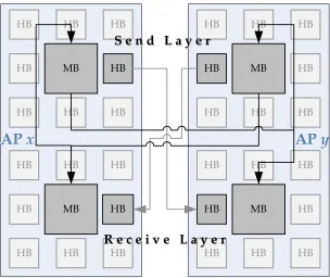
From a hardware point of view, communications use eight handshake buffer pairs,

which are used to exchange handshake codes, as shown in Table 2.3, and two message

buffers, which are used to exchange messages, as shown in Figure 2.3. The transfer of a

message from atomic processorxto atomic processoryis called hereafter a communication

cycle, and is illustrated graphically in Figure 2.4. It proceeds as follows:

1. Atomic processoryresets its receiving handshake buffer once it is ready to receive a

handshake code. This does not mean it is ready to receive a message yet.

2. Atomic processorxrepeatedly checks the receiving handshake buffer of atomic

pro-cessory. When it sees that the latter has been reset, it uploads the handshake code of

the message it wants to send.

(27)

handshake codes it may have received from other neighbors. This comparison is used

to prioritize transfers, where handshake code 1 in Figure 2.6 has the highest priority.

Once it is ready to receive the message from atomic processorx, atomic processory

resets its receiving handshake buffer again.

4. Atomic processorxchecks repeatedly the receiving handshake buffer of atomic

pro-cessory. When it sees that it has been reset again, it transfers the message into the

message buffer of atomic processory.

HB HB HB HB MB HB HB HB HB HB HB HB MB HB HB HB HB HB HB MB HB HB HB HB HB HB MB HB HB HB HB HB HB HB HB HB S e n d L a y e r

S e n d L a y e r

R e c e i v e L a y e r

[image:27.612.162.466.289.545.2]

AP x

AP

x

AP y

AP

y

Figure 2.3: The communications hardware is divided into a send and receive layer. Each layer uses a set of 8 handshake buffers and one message buffer. This allows full-duplex message passage.

The handshake code received by an atomic processor is used for two purposes: first, to

prioritize transfer requests received in the same cycle from different neighbors, and second,

(28)

[image:28.612.99.521.182.616.2]

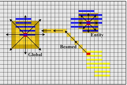
Table 2.3: Communications handshake codes.

Code Operation Description

0 (0000) AP is ready The atomic processor is ready to receive the next

hand-shake code.

1 (0001) Global cast The message has to be propagated throughout the entire

sea of atomic processors.

2 (0010) Beamed cast The message has to be propagated to a specific location

in the sea of atomic processors.

3 (0011) Entity cast The message has to be propagated only inside an entire

entity; the propagation of the message will end at the edge of the entity.

4 (0100) Local cast The message has to be sent only to the atomic

proces-sor’s eight neighbors.

5 (0101) P2P cast The message has to be sent only to a single neighbor.

6 (0110) Function

Definition Move request

The message is a P2P cast, in which a function defini-tion element request to move into a neighboring atomic processor.

7 (0110) Function

Instance Move request

The message is a P2P cast, in which a function instance element request to move into a neighboring atomic pro-cessor.

8 (0110) Data Structure

Move request

The message is a P2P cast, in which a data structure element request to move into a neighboring atomic pro-cessor.

9 (0111) Abut request The message is a P2P cast, in which an abutment

be-tween two associated entities is requested.

10-14 Reserved Reserved for future expansion

15 (1111) AP is not

functional

(29)

APx checks APy receiving

HB for zero APy resets its

receiving HB

APx uploads handshake code in APy receiving HB APx APy APy compares handshake code to determine priority

When it is ready to receive the message, APy resets again its HB

APx checks APy receiving

HB for zero

APx transfers message in

APy MB

t

Figure 2.4: A complete communications cycle. Atomic processorxis transmitting a

mes-sage to its neighbor, atomic processory.

which are shown in Table 2.3. Code 0 indicates the atomic processor’s readiness to accept

the next handshake code from its neighbor. Codes 1-5 encode the five different cast types.

Codes 6-8 are used during the move process, and code 9 is used during the abut process.

Code 15 is used to indicate that the atomic processor is not functional. The remaining codes

are currently reserved for future extensions.

Each of the two communication layers shown in Figure 2.3 comprises one set of

hand-shake buffers and one message buffer. Thus, an atomic processor can receive and send a

message at the same time. This eliminates the possibility of lockup if both atomic

proces-sors try to send a message to each other at the same time.

To avoid duplicate transmissions of the same message to the same atomic processor,

during a global, or beamed, or entity cast, a message is routed according to the scheme

presented in Table 2.4. For example, if the message is received from the neighbor to the

north, it is sent to the south, southeast and southwest neighbors. Messages received from

east, south and west are routed in a similar way. Alternatively, if for example the message

is received from the neighbor to the northeast, it is sent to the southwest neighbor only.

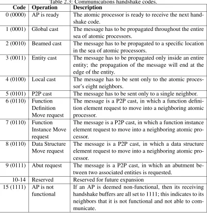
The routing and propagation of a global cast message is shown in Figure 2.5. This is also

applicable to an entity cast, except the propagation stops at the edge of the entity. The

(30)

casts are shown in Figure 2.6. In a beamed cast, the maximum number of atomic processors

the message has to pass through is equal to max{|xs−xr|,|ys−yr|}, where xs, ys, xr,

andyr are the(x, y)coordinates of the sending and receiving atomic processors.

Table 2.4: Message routing scheme used during a global or entity casts.

Receive From Transmit To

N NE E SE S SW W NW

N 4 4 4

NE ₄

E ₄ ₄ ₄

SE 4

S ₄ ₄ ₄

SW 4

W ₄ ₄ ₄

NW ₄

We have identified the need for two message formats, as shown in Table 2.5a and 2.5b.

A type 0 or result message is entity cast either by a function instance element or a data

structure element. The former entity casts it after it has executed its instruction. The latter

entity casts it during the execution initialization phase, which follows the abutment with

the associated function instance. Message types are described in Table 2.6, and their usage

(31)

Beamed

Global

[image:31.612.109.515.219.490.2]

Entity

Figure 2.5: Routing and propagation of a beamed, entity, and global cast messages. In a beamed cast, the maximum number of atomic processors the message has to pass through

is equal tomax{|xs−xr|,|ys−yr|}, where the sender is at(xs, ys)and the receiver is at

(32)

Desired Path Desired Path

Alternate Path Alternate Path Moving Entity

Element Moving Entity

Element

Target AP for Abutment

[image:32.612.107.514.231.499.2]

Target AP for Abutment

(33)

Table 2.5: Message formats. The numbers of bits in the shaded boxes change with the size of the sea of atomic processors and/or size of operands. The message codes are described in Table 2.6. ID = Identification number; S = Source; D = Destination; I = Intermediate.

a) Result Message Format

Sea Size Message Type Message Source ID Result Value Primary/ Secondary Operand Execution Order Number Status Bits Reserved Total Bits

64K 4 16 32 32 16 8 20 128

1T 4 40 64 64 40 8 44 256

b) Message Formats for types 1-11

Sea Size Message Type Message Source ID Message Dest. ID Intermediate ID ID Type: S/D/I Reserved Total Bits

64K 4 16 16 16 2 / 2 / 2 70 128

1T 4 40 40 40 2 / 2 / 2 126 256

2.4

Entity Movement

An entity element moves from atomic processorxinto atomic processoryas follows:

1. Atomic processor x requests to move an entity element into atomic processoryby

setting its handshake buffer to code 6, if the element is a function definition element,

or to code 7 if the element is a function instance element, or to code 8 if the element

is a data structure element, as described in Table 2.3.

2. Atomic processoryresets its handshake buffer back to 0 if it is ready to receive the

new element. It can only do so if it is not storing any other similar entity element.

3. Once the move request is accepted, atomic processorx transfers the entity element

information through the message buffer.

The move is further triggered and sustained through the use of theMove to Abut

(34)

function instance element in the 64K and1T seas of atomic processors, 274 bits and 538

bits, respectively, have to be transferred. The size of the message buffers being 128 bits

and 256 bits, respectively, three transfers through the message buffer are necessary, and

therefore steps 1 - 3 are repeated three times for these kinds of elements. A data structure

element needs to transfer 148 bits and 276 bits, respectively, and therefore steps 1-3 are

executed twice.

In the course of a move, an entity element may encounter unavailable atomic

proces-sors. In this case, it first moves in an alternative direction, and then corrects its course by

moving again towards the target location. For example, in Figure 2.6 the moving entity

element encounters an unavailable atomic processor to the southeast. Then it tries the next

counterclockwise neighbor. In the example, the neighbor to the east is available, and it

moves into it. Then it tries again to move southeast but encounters another unavailable

atomic processor. Thus, it tries the next counterclockwise neighbor, and so on. Finally,

after five moves due east, it can turn southeast and move towards the target direction. If the

front of the moving entity gets stuck, the back is forced to move around and become the

new front. Thus, entities will not get stuck during moves.

2.5

Input/Output

Two special kinds of moves are the input and output of entities into the sea of atomic

processors. These occur through atomic processors which are connected to the input /

output ports, illustrated in bold in Figure 2.1. The input of function definition entities is not

time critical. Thus, it can be performed serially, following the steps illustrated in Figure 2.7.

As for data, the amount and speed to be input and/or output are application dependent. In

these cases, an entity may transfer via several input / output ports and associated atomic

(35)

[image:35.612.107.513.102.641.2]

Table 2.6: Message codes and descriptions for non-result message types.

Code Function Description

0x0 Result The result entity cast by a function instance element after it has executed its instruction; or by a data structure element during the initialization phase, following abutment with the associated func-tion instance.

0x1 Instantiate Function

Beamed cast by a function instance element executing a CALL in-struction; it instructs the function definition, if it exists, to create a function instance of itself in the execution layer; after it has been created, the latter moves away, abuts with the data structure it has to process, and commences execution.

0x2 Instantiate Function (Interrupt)

Similar to 0x01, except the source of the call is an interrupt source.

0x3 Return Value Beamed cast by the called function instance to the calling function instance, after it has completed execution.

0x4 Return Value (Interrupt)

Similar to 0x03, except the returning function is an interrupt service routine.

0x5 Move to Abut Triggers elements of an entity to continue moving to abut. 0x6 Abutment

Completed

Entity cast by a function instance element once it has abutted with an element of the associated data structure entity.

0x7 Terminate Function Instance Entity

Entity cast by the function instance element that executes the RE-TURN instruction, after it has beamed cast the return value. 0x8 Request Location

of Function Definition

Global cast by a function instance element executing a CALL in-struction; it requests the(x, y)Coordinates or Hardware ID of the function definition it wants to call.

0x9 Acknowledge Location of F.D.

Beamed cast by a function definition element in response to 0x8. 0xA Request Location

of Data Structure

Global cast by a function instance element executing a CALL in-struction; it requests the(x, y)Coordinates or Hardware ID of the data structure the called function will have to process.

0xB Acknowledge Location of D.S.

Beamed cast by a data structure element in response to 0xA

A) B) C) D) E)

Figure 2.7: An entity enters the sea of atomic processors, when viewed from a → f, or

exits the sea of atomic processors, when viewed fromf → a. Large entities may be input

(36)

2.6

Entity Abutment

After moving diligently towards the target location, at some point a function instance

ele-ment encounters a data structure eleele-ment. The function instance eleele-ment initiates an abut

request, using handshake code 9 and a point-to-point cast, and provides its entity

identifica-tion number. In return, the data structure element provides its entity identificaidentifica-tion number.

If the identification numbers match, the function instance element, entity casts an abutment

complete message, type 6 in Table 2.6. Because the move and abutment processes are

asynchronous, multiple function instance and data structure elements may abut at the same

time, so multiple abutment complete messages may be entity cast. The function instance

entity abutted to its associated data structure entity will hereafter be called a superentity.

Once they receive the abutment complete message, all data structure elements entity cast

their current data word values over the superentity. These are then received by all function

instance elements which have to update their primary and/or secondary operand values.

This means that before execution commences, all function instance elements have their

operands available, less the values updated at runtime.

2.7

Instruction Execution

Once abutment completes, and all data structure elements entity cast their data word

val-ues, the first instruction executes as soon as it has its operands available. At run-time, all

function instance elements monitor all entity casted result messages. If the message source

identification number matches one of their own source identification numbers, they update

their primary operands, and/or secondary operands, and/or source status bits values. At

the same time, they check theExecutionOrdernumber in the result entity cast message. If

(37)

all operand and source status bits values are available, the function instance element

ex-ecutes the instruction. TheExecutionOrder andPrevExecutionOrder numbers, which are

statically assigned, are the means through which the architecture implements the necessary

execution flow control. The operand values, source status bits values and ExecutionOrder

number may arrive in the same or different result entity cast messages, and in arbitrary

order. The instruction cycle completes when the function instance element entity casts the

result of its instruction execution.

There are obviously no structural dependencies. Data and control dependencies are

explicit, and therefore automatically resolved. Instruction level parallelism is exploited

dynamically and it is maximized, because an instruction executes as soon as it has its

operands, source status bits, and knowledge of the fact that the previous instruction in

the execution flow has executed.

At runtime, all result messages are entity cast over the entire superentity, and so also

reach all data structure elements. A data structure element updates its data word value

when there is a match between the message source identification number and its element

identification number. This means that when the function instance completes execution and

is ready to return the data structure, the latter is up to date.

All instructions defined in Table 2.2 execute as described above, except for CALL and

RETURN, which are described in the next section.

2.8

Function Calls

A function call involves four entities: the calling function instance, the called function

definition and its instance, and the data structure to be processed. A complete function call

and return cycle comprises the following steps:

(38)

function definition Y of the called function to create an instance of itself, which

should move to location(xZ, yZ)and process data structureZ. If the calling function

instance X knows the location of the function definitionY, it uses a beamed cast.

Else, it uses a global cast. In either case, it provides its own(xX, yX)coordinates.

2. Function definition Y replies with a beamed cast, in which it provides its current

coordinates and a confirmation that the function instance Yi has been created and

moves towards data structure Z. Function definition Y instantiates Yi by

simulta-neously creating a copy of its elements from the definition layer into the execution

layer.

3. Function instance Yi moves to, abuts with, and processes data structure Z, as

de-scribed in the previous four sections.

4. The last instruction executed by function instanceYi is a RETURN. The element of

function instanceYi that executes the RETURN, beam casts areturn valuemessage,

see Tables 2.5 and 2.6, to the calling function instanceX. It also entity casts a

termi-nate function instance entitymessage, if the function instance is no longer needed.

During the entire call-return cycle, the element of function instanceXthat executes the

CALL instruction cannot move, because it has to receive the RETURN beamed cast.

Mul-tiple CALL instructions may call for mulMul-tiple instantiations of the same function definition,

to process different, independent data structures.

Input / output port requests or interrupts are handled in the same way, except for the

fact that the calling function is actually an input / output port. If and which currently

run-ning function instances are halted, or affected by the exception, is decided by the function

(39)

2.9

Loops

If there are no data and/or control dependencies between the iterations of a loop, they

are executed concurrently, as shown in Figure 2.9a. In this case, each loop iteration is

implemented by a separate set of elements or function instance entities. These iterations

complete out-of-order and the last instructions of all iterations will entity cast the same

ExecutionOrdernumber. This is received and counted by the first instruction after the loop.

When the count value is equal to the ExecutionCountvalue, it proceeds to execution and

the loop is completed. Double counting is eliminated because the same entity cast cannot

reach the same element twice, as is illustrated in Figure 2.8. If there are dependencies,

loop iterations have to be executed in sequence, as shown in Figure 2.9b. In this case, it is

not effective to create or instantiate elements or function instances for each iteration of the

loop. The single instance of the iteration is executed repeatedly. The last instruction in the

iteration, which can also manipulate the index, executes if the condition to repeat is true.

It entity casts theExecutionOrdernumber of the instruction before the loop, triggering the

instructions in the loop to execute again. The first instruction after the loop executes if the

condition to repeat is false. This is equivalent to a for loop in which the first iteration is

always executed. Alternatively, the condition can be tested by the first instruction of the

(40)

[image:40.612.132.492.192.558.2]

(41)

m-1

m

m+n

m+n+k+1

m+1

m+n+1

m+k

m+n+k

m+n+k+1

m-1

m

m+n-1

m+n m+n+1

m+n+2

a) b)

Last elements before the loop

Independent iterations of a loop execute concurrently

First elements after the loop

Loop dependent iterations of a loop execute sequentially

[image:41.612.99.520.215.514.2]

The last elements of each iteration of the loop

(42)

Chapter 3

Programming Environment and

Simu-lation Model

This chapter describes the model of the architecture, which was described in the previous

chapter. This model is used in the integrated development environment and simulator.

Furthermore, justification for several of the software design decisions are introduced here

and further discussed in Chapter 5. Finally, a short discussion has been provided describing

the creation of a function definition in the IDE.

3.1

Integrated Development Environment GUI

As our computing environments continue to look for ways to exploit more concurrency and

focus less on executing a sequential string of commands, programming these upcoming

massively parallel architectures is a challenge. Code development for a massively

paral-lel architecture such as the one discussed in Chapter 2, is a difficult task when presented

with the choice of the standard text based coding languages such as C, C++ and Visual

Basic, just to name a few, which primarily are sequential in nature. Much work has been

done to create concurrent programming languages in addition to using APIs such as the

(43)

languages [77–79]. An alternate approach is a compiler designed to automatically extract

parallelism from sequential code, but such compilers have very limited success and are

typically aimed toward specific applications [80]. Many of these parallel programming

techniques are designed for a limited number of processors or processors that are far more

complex then the RISC processors in the architecture examined in this research. Because

of this, an alternate programming method and environment are required.

Hence, an initial approach at programming the massively parallel architecture was

at-tempted using a C like, text based format. It was quickly discovered that this format was

cumbersome and lacked an easy way to convey important information, such as program

flow control. Each time a change was desired, even in a simple program, it had to be made

in several locations throughout the code. In anything more than a simple algorithm this

meant that thousands of lines of code would have to be browsed through. Figure 3.1 shows

an example of this text based code for one of the example algorithms discussed later.

Ulti-mately, the limitation of a text only programming language is that text conveys sequential

information.

In contrast, a graphical programming environment allows for multiple threads of a

pro-gram to be displayed simultaneously. An example of this is provided by Mathworks’

Simulink, in which several dynamic systems can be graphically diagrammed within the

same project. While Simulink offers several libraries for control theory and digital signal

processing, its use in implementing a programming environment for a massively parallel

computer architecture would require the development of a custom library and significant

add-ons. Similarly, one of the several commercially available schematic capture programs

would serve adequately for diagramming the model of a massively parallel program.

How-ever, these tools would still require an add-on for simulation purposes.

Furthermore, programming tools provided forfield programmable gate arrays(FPGAs)

(44)

PXOWLSOLHUW[W %HJLQ&RQFXUUHQW >,QSXW ([HFXWLRQ2UGHU ([HFXWLRQ2UGHU&RXQW ([HFXWH$IWHU2UGHU 6WDWXV%LWV6RXUFH

6WDWXV%LWV9DOXHV & )DOVH1 )DOVH9 )DOVH= )DOVH &RQGLWLRQDO([HFXWLRQ 8QFRQGLWLRQDO

3ULPDU\2SHUDQG6RXUFH

3ULPDU\2SHUDQG7\SH 8QVLJQHG,QWHJHU 3ULPDU\2SHUDQG9DOXH

6HFRQGDU\2SHUDQG6RXUFH 6HFRQGDU\2SHUDQG7\SH 6HFRQGDU\2SHUDQG9DOXH

2SHUDWLRQ 1238QFRQGLWLRQDO

&DVW (QWLW\,GHQWLILFDWLRQ1XPEHU([HFXWLRQ2UGHU1XPEHU 6WDWXV%LWV3ULPDU\2SHUDQG @ >,QSXW ([HFXWLRQ2UGHU ([HFXWLRQ2UGHU&RXQW ([HFXWH$IWHU2UGHU 6WDWXV%LWV6RXUFH

3ULPDU\2SHUDQG6RXUFH

6HFRQGDU\2SHUDQG6RXUFH 6HFRQGDU\2SHUDQG7\SH 6HFRQGDU\2SHUDQG9DOXH

2SHUDWLRQ 1238QFRQGLWLRQDO

&DVW (QWLW\,GHQWLILFDWLRQ1XPEHU([HFXWLRQ2UGHU1XPEHU 6WDWXV%LWV3ULPDU\2SHUDQG @ (QG&RQFXUUHQW >$WRPLF3URFHVVRU ([HFXWLRQ2UGHU ([HFXWLRQ2UGHU&RXQW ([HFXWH$IWHU2UGHU 6WDWXV%LWV6RXUFH

3ULPDU\2SHUDQG6RXUFH L 3ULPDU\2SHUDQG7\SH 3ULPDU\2SHUDQG9DOXH 6HFRQGDU\2SHUDQG6RXUFH

6HFRQGDU\2SHUDQG7\SH 8QVLJQHG,QWHJHU 6HFRQGDU\2SHUDQG9DOXH

2SHUDWLRQ $1'8QFRQGLWLRQDO

&DVW (QWLW\,GHQWLILFDWLRQ1XPEHU([HFXWLRQ2UGHU1XPEHU 6WDWXV%LWV3ULPDU\2SHUDQG @ %HJLQ&RQFXUUHQW >$WRPLF3URFHVVRU ([HFXWLRQ2UGHU ([HFXWLRQ2UGHU&RXQW ([HFXWH$IWHU2UGHU 6WDWXV%LWV6RXUFH

3ULPDU\2SHUDQG6RXUFH

6HFRQGDU\2SHUDQG6RXUFH L 6HFRQGDU\2SHUDQG7\SH 6HFRQGDU\2SHUDQG9DOXH

2SHUDWLRQ $''36=

&DVW (QWLW\,GHQWLILFDWLRQ1XPEHU([HFXWLRQ2UGHU1XPEHU 6WDWXV%LWV3ULPDU\2SHUDQG

[image:44.612.108.506.88.662.2]

3DJH

(45)

Xilinx exhibit similar problems. Logical models of processors in the proposed architecture

could be created in these tools and simulated, but computing needs would be excessive. The

shortcomings of these tools leads to the conclusion that a custom environment is needed.

Moreover, a common textbook approach to modeling a parallel program is the

depen-dency graph [81]. A typical dependency graph shows the dependencies between objects and allows one to determine the order or lack of order that the objects must be evaluated in.

This method is often used to aid in decisions about the appropriate program flow in

concur-rent algorithms. The proposedintegrated development environment (IDE) allows the user

to indicate concurrency and dependencies of each processing element for a given function

or set of functions in a manner similar to a dependency graph.

Once the programmer considers an algorithm complete, the option is provided to parse

the visual display and check for errors as well as provide warnings about potential mistakes.

If the program is parsed without any errors, the program is simulated using a simulation

engine designed to match the proposed architecture. The simulator does not account for

communication delays between processors as would exist in actual hardware because of the

large amount of resources required for this type of simulation. Instead, the communication

latency is assumed to be zero, allowing for a purely functional simulator used for algorithm

development. This is similar to how one may functionally simulate VHDL or Verilog code

without hardware timing delays to get an idea of how a given algorithm works. Henceforth,

the combined IDE and simulator will be referred to as the IDE for the remainder of the

document.

The goals set forth for the prototype IDE are to show proof of concept for the proposed

visual programming method and to functionally simulate simple algorithms, intended

pri-marily for embedded applications, on the proposed architecture. A typical embedded

appli-cation may differ from a desktop or server system in that it often has real time constraints

(46)

these applications also quite frequently require that system memory and power

consump-tion are kept to a minimum. In many cases, the only system memory is part of the processor

chip itself [2]. One example of an embedded application is a cell phone; it requires real

time processing of radio signals in a small, low-power package.

Accordingly, the user interface is intended to mimic a dependency graph in some

re-gards and is based on a layout grid that the user can place tokens onto. The grid is arranged

such that when the user places a token, it will snap to that grid location automatically. The

grid is divided into rows and columns. A token is assigned an(x, y)location based on the

row and column into which it has been placed. Each row signifies a concurrent step to be

simulated so that all tokens on a given row execute in parallel. Columns provide no

signif-icance in the user interface beyond allowing each token to be assigned a unique location

on the grid. There are several types of tokens that can be placed on to the layout grid. The

token types include atomic processors (APs), data elements (DEs), function calls (Fns),

inputs,sequential arrays(SAs) andconcurrent arrays(CAs). The different types of tokens will be discussed in more detail later in this chapter, but for the purpose of this description,

each token represents a single atomic processor, with the exception of the array tokens.

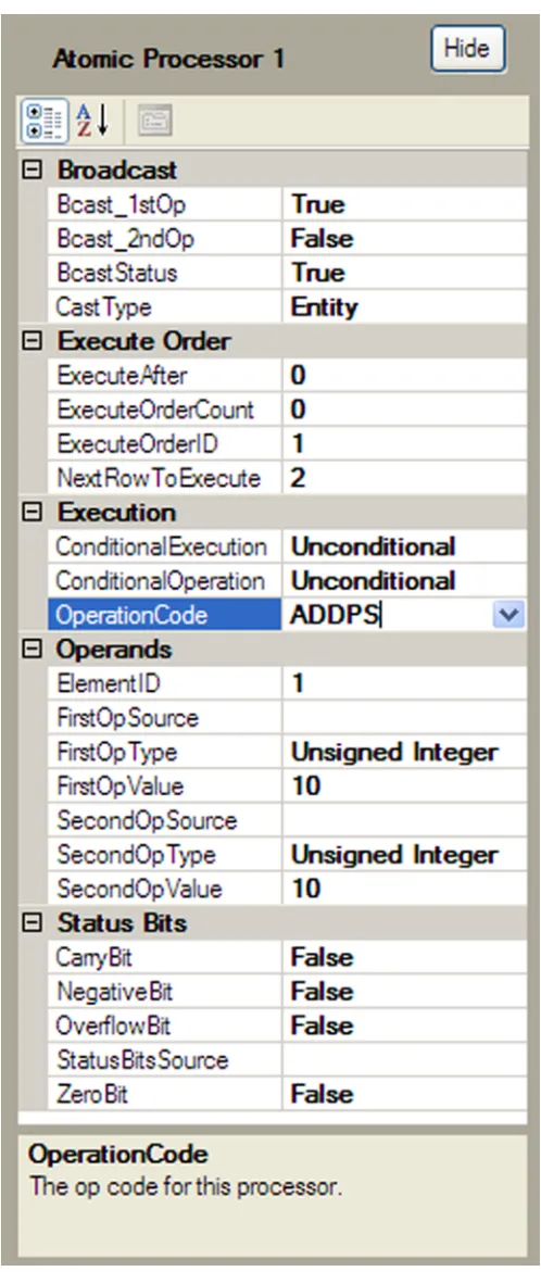
Once tokens are placed onto the design grid, properties for each token can be defined

in a table, called the property grid as shown in Figure 3.2, by selecting the desired token.

If a user indicates that a token should take one of its operands from another token, a line is

drawn connecting the two tokens to indicate the data dependency. Additionally, information

defining a processor’s operation code, status bits, execution order and broadcast type are

editable from the property grid. Currently, the execution order and broadcast information

have no effect on the simulator, due to the exclusion of communication delays from the

functional simulator and the implied program flow of the IDE’s graphical user interface

(GUI). If the IDE was further developed to compile code for a communication accurate

(47)

[image:47.612.185.434.88.679.2]

(48)

avoid the tedious and error prone process of populating them by hand.

3.2

Model of a Processor

Each processor is modeled by a single token placed on the layout grid. The basic building

block of the architecture, an atomic processor, is modeled by an AP token. Each AP token

is capable of performing a single arithmetic, logic, status bit or function return operation

as discussed in Chapter 2. Function calls, while represented by a standard operation code

are handled by a separate token in the IDE. An AP token provides the user with fields for

primary and secondary operands which can be defined within the token by providing a type

and value or received from another token on the layout grid. Status bit value and source

fields are also provided to allow for conditionals within the token. As with operands, if

another token is provided as a source for the status bits its values will override the internal

values.

Additionally, conditional tokens can be used to make program flow decisions based on

status bits passed from other processors or as defined within a processor. When a token

is made conditional, by defining a condition in its property grid, it will change to yellow

and display a conditional symbol on the face of the token. During a simulation conditional

tokens change color based on the program flow. If a conditional token executes, it becomes

green. If it does not execute, it becomes red.

Furthermore, there are two types of conditionals in the simulator:conditional execution

andconditional operation. Conditional executionblocks the broadcast of any information

from the token in the event the condition is not met. Conditional operationis non-blocking

and allows a broadcast of information from the token, but does not perform the indicated

operation on the operands when the condition is not met. A falseconditional operationis

(49)

Finally, other fields included for an AP fall into categories of broadcast information and

execute order fields. These fields are provided to the user solely for the export to human

readable text function of the IDE. They have no effect on the simulator which handles

execution order and message passing internally.

3.3

Specialty Tokens

In addition to the standard AP tokens, five other token types are available to the user,Input

Tokens, Function Calls, Data Elements, Concurrent Arrays and Sequential Arrays. The different token symbols are shown in Figure 3.3. Input tokens are added to the IDE through

the view menu by selecting the project properties dialog, currently the number of input

tokens is limited to ten. Input tokens do not represent physical processors in hardware, but

are a means for debugging a function definition during its development. Default values are

provided by an input token so a function definition can be simulated without instantiating it

from another Pond project. When a function definition is instantiated from another project

the default values provided by the input token are instead overridden by values being passed

into the function instance. Input tokens only provide fields for the default operand value

and type, and input description and label fields to aid the user in selecting the proper inputs

during a function call.

The remaining token types are added to the IDE the same way AP tokens are added,

through the left hand side tool bar, shown to the left of Figure 3.3. Function call tokens

allow the user to instantiate a function definition from within a project. Each function call

token has a field for the .pnd file that the function definition is stored in. Upon populating

this field, the file is read and the appropriate number of input source fields show up in

the property grid interface for the user to define. Each input source field provides a label

(50)

[image:50.612.104.518.142.625.2]

(51)

method of calling functions differs from the actual description of how a function is called

in hardware, which requires a normal atomic processor with the function to instantiate in

the primary operand field and a reference to the data structure of data elements with the

function inputs as the second operand, this seemed impractical in the IDE. The primary

reason for this decision was the lack of a way to use a file name as a primary operand in an

atomic processor, and a still-to-be-determined way to define or reference a data structure

in the IDE. Overall thefunction calltoken still models what happens in hardware from the

underlying simulation engine by instantiating a function definition and providing it with

data to process. When a function instance reaches its return token, the function call token

is provided with the returned operand to pass as an output to the rest of the project that

called the function.

Data element tokens represent entries within a data structure as defined by the archi-tecture in Chapter 2. Each data element has fields for first operand source, value, and type.

Each is capable of providing data to other tokens or receiving data from a source token.

Currently, the sequentialand concurrent array tokens have no function in the simulator,

they have been left for a future implementation of the IDE. The original thought behind the

array tokens was to allow the user to represent several tokens performing the same

opera-tion with only a single token, thus reducing the amount of time spent placing replica tokens

on the layout grid. Each array token has an array size field and operand source index fields

in addition to the standard AP fields. These fields would allow the user to indicate the

number of tokens in the array and how to process source inputs to the array, respectively.

3.4

Simulator Basics

When a simulation is started by the user by selecting simulate under the tools menu or

(52)

is parsed. During the parsing process, each token’s properties are read in and checked for

errors. If an error is found during parsing, an error list is returned to the user indicating the

problem. Warnings can also be returned to the user indicating a potential problem, but do

not stop simulator execution. If a token’s information is successfully read in without errors,

a simulation operation for that token is created. Once an entire row is parsed successfully

without errors, a simulation step that contains each of the simulation operations for that

row is created. An overall simulation path is assembled from steps that represent each row

of the layout grid, as further discussed in Section 5.1.3.

Likewise, during simulation, the simulator calls the step for each row, which in turn

calls the operation for each token. Operations are split intomath,logic,status,no,function

andcalloperations. Themathandlogicoperations are called if an operation code defined

in a token is an arithmetic or logic type operation. Statusoperations are called for

manipu-lations to status bits andnooperations are called if a NOP is desired. Functionoperations

handle returns from a function instance and call operations handle function instantiation

calls.

Furthermore, the simulator can run all the steps at once or an option is provided to step

through them one at a time. Breakpoints are provided for the simulate all option to stop

simulator execution at a desired location. Additionally, during the simulate step option,

or at a breakpoint, a yellow bar highlights the current row. Once the user has finished

simulating their design they can return the IDE to design mode by selecting theDMbutton

on the right hand side tool bar. Further details about the simulator internals are provided in

(53)

3.5

Creating a Function Definition

Now that a basic understanding of the IDE exists, it is possible to create simple function

definitions. A function definition consists of an appropriate number of input tokens to pass

data into the function instance and tokens on the layout grid to process data. The user

may set the number of inputs for the function definition and define name and description

fields for the function from within the project properties dialog. In addition the user can

select the bit size representation for the project; options of 16, 32, or 64 bit operands are

available. The function definition ends in an AP token with the “RETURN” opcode as its

operation. Once a function definition is completed and saved, it can be ins

Pond IDE: Machine level program development environment and register transfer level simulator for a massively parallel computer architecture