Non-linear predictive generalised minimum variance state-dependent control

(1)

Nonlinear Predictive GMV

State-Dependent Control

Michael John Grimble

1

_{and Pawel Majecki}

2

1

Industrial Control Centre, Dept. of Electronic and Electrical Engineering, University of Strathclyde,

204, George Street, Glasgow, G1 1XQ, UK (phone: +44(0)1415482378; e-mail: [email protected])

2_{Industrial Systems and Control Ltd, Culzean House, 36 Renfield Street, Glasgow, G2 1LU, UK.}

(e-mail: [email protected])

Abstract

A Nonlinear Predictive Generalized Minimum Variance control algorithm is introduced for the control of

nonlinear discrete-time state-dependent multivariable systems. The process model includes two different types of

subsystems to provide a variety of means of modelling the system and inferential control of certain outputs is available. A state-dependent output model is driven from an unstructured nonlinear input subsystem which can include explicit transport-delays. A multi-step predictive control cost-function is to be minimised involving weighted error, and either absolute or incremental control signal costing terms. Different patterns of a reduced number of future controls can be used to limit the computational demands.

Keywords: optimal, state-dependent, predictive, nonlinear, minimum-variance.

Acknowledgements: We are grateful for the discussions and cooperation with Professor Yan Pang (Dalian

University of Technology) on the development of the algorithms.

1. Introduction

The objective is to design an industrial controller for nonlinear and state-dependent, or linear parameter varying

systems, which has some of the advantages of the popular Generalised Predictive Control (GPC) algorithms.

(2)

to be similar, however the output subsystem is assumed to be represented in state-dependent, possibly unstable, form.

The multi-step predictive control cost-function to be minimised involves both weighted error and control costing terms, which can be used with different error and control horizons. Two alternative types of control signal input to the plant model are considered. The first is the traditional control signal input and it is this signal which is also penalized in the predictive control criterion. However, as is well know it is sometimes desirable to augment the plant model with an integrator to provide a simple way of introducing integral action. In the augmented system the new system input is the change of control action or increment, and in this case this is the signal which should be penalized in the criterion. The results will apply to both cases and a parameter change between β = 0 and β =

1 will provide the necessary switch. The cost includes dynamic weightings on both error and control signals.

There is a rich history of research on nonlinear predictive control ([2] to [7]), but the development proposed is somewhat different, since it is closer in spirit to that of a model based fixed-structure controller for a time-varying system. Part of the plant model can be represented by a very general nonlinear operator and the plant can also include a state-dependent (or linear parameter varying) output sub-system model, rather than a LTI model, as in previous work.

For equivalent linear systems, stability is ensured when the combination of a control weighting function and an error weighted plant model is strictly minimum phase. For nonlinear systems it is shown that a related operator equation is required to have a stable inverse. The dynamic cost-function weightings are chosen to satisfy performance and stability/robustness requirements and a simple method is proposed for obtaining initial values for the weightings.

2. Non-linear Operator and State-Dependent System

The plant model can be nonlinear, dynamic and may have a very general structure. The output subsystem and disturbance model is represented by a so-called state-dependent sub-system in Fig. 1. The plant involves two

nonlinear subsystems and the first is of a very general nonlinear operator form and written as follows:

(

)( )

(

₁

)( )

1

k k

u t =z− u t

 

(3)

Fig. 1: Feedback Control with Inferred or Controlled Outputs

2.1 Signal Definitions

The output of the system to be controlled y(t) may be different to that measured, as shown in Fig. 1, and this output includes deterministic d(t) and stochasticy td( )components of the disturbances. The measured output ym( )t also

includes deterministic dm( )t and stochastic ydm( )t components of the disturbances. The stochastic component is

modelled by a disturbance model, driven by zero mean white noise{ζ₀( )}t . The measurement noise

{

v t

_m

( )}

is assumed to be zero-mean white noise with covariance matrix T 0

f f

R =R ≥ . There is no loss of generality in assuming that

{

ζ₀( )t

}

has an identity covariance matrix. The controlled output must follow a referencer t( ), which is assumed to be known.

2.2 State-Dependent Sub-System Models

The second or output subsystem is in a state-dependent/LPV form, which includes the plant and the error weighting models (see [8]). This is assumed to include a common k-stepstransport delay, and has the state-equation:

x t0( + =1)



0( ,x u0, ) ( )p x t0 +



0( ,x u0, )p u t k0( − +)



0( ,x u0, )p

ζ

0( )t +



0( ,x u0, )p d0d( )t (1) where the vector p is a vector of known variables like speed of an engine, or altitude of an aircraft that change with operating conditions. The controlled output and measured outputs (without measurement noise):

y t( )=d t₀( )+₀( ,x u₀, )p x t₀( )+₀( ,x u₀, )p u t k₀( − )₍₂₎ y t_m( )=d₀_m( )t +₀_m( ,x u₀ ₀, )p x t₀( )+₀_m( ,x u₀ ₀, )p u t₀( −k) (3)

y

+

0 d

d = +d y

+ +

+

+ +

m

y

Controlled Output

0m m dm

d =d +y

Noise

m

v

r _u

ζ

0

C

Nonlinear operator subsystem

0

u

State-dependent subsystem Measurement or observations signal z_m

Disturbances

0



0d

d

1k



(4)

where 0

0( )

n

x t ∈R .

This model can be a function of the states, inputs and parameters( ( ),x t u0(t−k), ( ))p t . The deterministic component of the input disturbance is d₀_d( )t and the disturbance on the output to be controlled

0( ) ( ) d( )

d t =d t +y t includes a known deterministic component d t( ) and a stochastic componenty t_d( ). The disturbance on the measured outputd₀_m( )t =d t_m( )+y_dm( )t , where dm( )t is deterministic and ydm( )t is stochastic.

The plant includes a disturbance model on the output, driven by zero mean white noise ω(t): ( 1) ( ) ( ), ( ) nd

d d d d d

x t+ =



x t +



ω

t x t ∈R (4)

y td( )=



dx td( ) and ydm( )t =



dmx td( ) (5) The signals of interest include the error on the output to be controlled and the measured output:

Error signal: e t

( ) ( ) ( )

=r t −y t (6)

Observations signal: zm

( )

t =ym

( )

t +vm

( )

t (7)

The signal to be controlled will involve the weighted tracking error in the system:

x t_p( + =1)



_px t_p( )+



_p

(

r t( )−y t( ) ,

)

( )

np

p

x t

∈

R

(8)

e tp( )=px tp( )+p

(

r t( )−y t( )

)

(9)

The traditional method of introducing integral action in predictive controls is to augment the system input by adding an integrator using the input sub-system:

x ti( + =1)

β

x ti( )+ ∆u₀(t−k), ( ) i

n i

x t ∈R (10)

u t0( −k)=βx ti( )+ ∆u t0( −k)

1 1 0

(1

β

z− )− u (t k)

= − ∆ − (11)

The_{ }(1_z1)_{, for}_β ₌₁_{and the transfer (11) is an integrator without additional delay, and if}_β ₌₀_{, then}

0( ) 0( )

u t−k = ∆u t−k . The results can therefore apply to systems using control input or rate of change of control.

2.3 Total Augmented System

(5)

( ) 0( ) ( ) ( ) ( )

T

T T T T

d i p

x t = x t x t x t x t _

To simplify notation write



_t =

(

x t u t k p t( ), 0( − ), ( )

)

and similarly for the time-varying matrices

, , and

  t t t t, with state

( )

n

x t

∈

R

. The augmented system equations may be written as follows:

x t( + =1) _tx t( )+ ∆_t u t₀( − +k) _tξ( )t +d t_d( ) (12) y t( )=d t( )+



tx t( )+ ∆



t u t0( −k) (13)

( ) ( ) m ( ) m ₀( )

m m t t

y t =d t +



x t +



∆u t−k (14)

( ) ( ) ( ) ( ) 0( )

m m

m m m t t

z t =v t +d t +



x t +



∆u t−k

(15)

e tp( )=dp( )+t p tx t( )+p t∆u t0( −k) (16) The augmented system has an input ∆u t₀( ) and the change in actual control is denoted∆u t( )

0 1

(these are related as∆u t( )=



_k

(.,.)

∆

u t( )).

2.4 Definition of the Augmented System Matrices

The equations in §2.2 can be combined with a little manipulation to obtain the augmented system matrices. That is the total state-equation model may be written in terms of the augmented system matrices, as follows:

0

( 1) _t ( ) _t ( ) _t ( ) _d( )

x t+ = x t + ∆u t−k + ξ t +d t (17) where the matrices in this equation are defined from the combined model equations:

0 0 0 0 0

0

0 0 0

( 1) 0 0 ( )

( 1) 0 0 0 ( ) 0

( )

( 1) 0 0 0 ( )

( 1) ( )

  



        

d d d

i i

p p p d p p p p

x t x t

u t k

x t I x t I

x t x t

β

β β

+

       

 ₊       

  ₌    ₊ _∆ ₋

 +       

 ₊  ₋ ₋ ₋    ₋ 

       

       

0 0

0 ( ) ( )

0 0

0 0 ( ) ( ( ) ( ))

0

0 0

d d

p

t d t

t r t d t

ζ ω

 

 

 _{ } _ _ _

 

+ _ _+ _ _

 

 _ _ _ − _

 

   

 





(6)

The output to be controlled may be written in terms of augmented system model in (13). That is: y t( )=d t( )+₀x t₀( )+_dx_d( )t +₀βx t_i( )+ ∆₀ u t₀( −k)

=d t( )+_tx t( )+ ∆_t u t₀( −k)

(19)

where _t =

[

 ₀ _d ₀β 0

]

and _t =₀ Similarly from (3) and (5), the measured output may be written in the augmented system as follows:

y t_m( )=d t_m( )+



_tmx t( )+



_tm∆u t k₀( − ) (20)

where _tm =

[

₀_m _dm ₀_mβ 0

]

and m ₀

t = m

 

Also from (2) and (9), the weighted tracking error to be minimised may be written as:

0

( ) ( )+ ( ) ( )

p p p t p t

e t =d t  x t + ∆u t−k

(21)

where d tp( )=p( ( )r t −d t( )), p t = −  p 0 − p d −β p 0 p and p t = − p 0. The subscript t on the state matrices here is used for the augmented system and in a slight abuse of notation it also indicates that these matrices are evaluated at time t, so that the system matrix at t+1 is written as_t₊₁.

3. State-Dependent Future State and Error Models

A state-dependent model prediction equation is required and later an estimator for the state-dependent models. The future values of the states and outputs may be obtained by repeated use of (12) assuming that the future values of the disturbance are known. Introduce the notation:

1 2...

i m

t m t i t i t m

−

+ = + − + − +

   

for i>m, where 0

t m+ =I

 for i=m

ti = t i+ −₁ t i+ −₂...t

for i>0, where 0

t =I

 for i=0

(22) Future states: Generalising this result obtain, fori≥1, the state, at any future timet i+ , may be written as:

(

₁ ₀ ₁

)

1

( )  ( )   ( 1 )  ( 1) ( 1)

i

i i j

t t j t j t j dd

j

x t i x t ₊− _{+ −} u t j k _{+ −}ξ t j d t i

=

+ = +

∑

∆ + − − + + − + + − (23)

where

1

( 1) ( 1)

i i j

dd t j d

j

d t i ₊− d t j

=

(7)

These equations (23) and (24) are valid for i≥0 if the summation terms are defined as null for i = 0. Noting (16) the weighted error or output signal e t_p( ) to be regulated at future times (fori≥0):

e tp( + =i) d tp( + +i)



p t i+ x t( + +i)



p t i+∆u t0( + −i k)

1 0

1

(

)

( )

(

1 )

pd

i

i i j

p t i t p t i t j t j j

d

t i

₊

x t

₊ ₊− _{+ −}

u t

j

k

=

+ +

 

+



∑

 

∆

+ − −

1 1 0

( 1) ( )

i i j

p t i t j t j p t i

j

t j u t i k

ξ

−

+ + + − +

=

+_

∑

_{ } + − +_ ∆ + − (25)

where d t_p( )=_p( ( )r t −d t( ))and the deterministic signals:

dpd(t+ =i) d tp( + +i) p t i+ddd(t+ −i 1) (26)

3.1 State Estimates Using State-Dependent Prediction Models

The i-steps prediction of the state for i≥0 and the output signals may be defined, noting (23), as:

₁ ₀

1

ˆ

(

| )



ˆ

( | )

 

(

1 )

(

1)

i

i i j

t t j t j dd

j

x t

i t

x t t

₊− _{+ −}

u t

j

k

d

t

i

=

+

=

+

∑

∆

+ − − +

+ −

(27)

where 1 2...

i j

t j t i t i t j

−

+ = + − + − +

    and

1

(

1)



(

1)

i i j

dd t j d

j

d

t

i

₊−

d t

j

=

+ − =

∑

+ −

, and for i = 0the ddd(t− =1) 0. The

predicted output:

y tˆ( +i t| )=d t( + +i)



_{t i}₊x tˆ( +i t| )+



_{t i}₊ ∆u t₀( − +k i) (28) The weighted prediction error for i≥0:

e tˆp( +i t| )=d tp( + +i)



p t i+ x tˆ( +i t| )+



p t i+∆u t0( + −i k)

(29) The expression for the future predicted states and error signals may be obtained by changing the prediction time in (27) t→ +t k. Then, fori≥0:

1 0 1

ˆ( | )  ˆ( | )   ( 1) ( 1)

i

i i j

t k t k j t k j dd

j

x t k i t ₊ x t k t _{+ +}− _{+ + −} u t j d t k i

=

+ + = + +

∑

∆ + − + + + −

(30)

(8)

0

ˆ ( | ) pd( ) ( ) ˆ( | )

i

p p t i k p t i k t k

e t+ +i k t =d t+ +i k + + + ∆u t+ +i  + + + x t+k t

1 1 0

( 1)

i i j p t i k t k j t k j

j

u t j

−

+ + + + + + −

=

+_

∑

_ _ ∆ + − (31)

and ˆ ( | ) pd( ) 0( ) ˆ( | )

i

p p t i p t i t k

e t+i t =d t+ +i  ₊∆u t+ − +i k  ₊₊ x t t ₁ ₀ 1

( 1 )

 i  i j

p t i t j t j

j

u t j k

−

+ + + −

=

+

∑

∆ + − − (32)

The deterministic signals in this equation:

1

( ) ( ) ( 1)

pd p

i

i j p t i k t k j d j

d t i k d t i k _{+ +} _{+ +}− d t k j

=

+ + = + + +

∑

  + + −

(33)

and for i = 0 the termdpd(t+k)=d tp( +k).

3.2 Vector Matrix Form of Equations

The predicted errors or outputs may be computed for controls in a future intervalτ ε[ ,t t+N] forN≥ 1. These weighted error signals may be collected in the following N+1 vector form:

1 2

ˆ ( ) ( )

ˆ ( 1 ) ( 1)

ˆ ( 2 ) ( 2) ˆ( | )

ˆ ( ) ( )

pd pd pd

pd t k

p t k p

p t k t k p

N p t N k p

I e t k d t k

e t k d t k

e t k d t k x t k t

e t N k d t k N +

+ + + + + + + + +   + +        _{+ +}   _{+ +}           + +  = + + + +                _{+ +}  _ _{+ +} _               1 2 0 1 0 2 0 0 ( ) ( 1) ( 2) ( )    

p t k

p t k N

u t u t u t u t N

+ + + + + + + ∆    _∆ ₊     ∆ +  +      _∆ ₊     0 1 0 1

2 1 2 1

0

1 2

1 2 1 1 0

0 0 0 0 ( )

0 0 0 ( 1)

0

0 0 ( 1)

0 ( )

 

    

       

p t k t k

p t k t k t k p t k t k

N N

p t k N t k t k p t k N t k t k p t k N t k N

u t u t u t N

u t N

+ + + + + + + + + + + + − − + + + + + + + + + + + + + + + − ∆        _∆ ₊          +   _∆ _{+ −}        _ _∆ ₊ _            (34)

Future error and predicted error: With an obvious definition of terms this equation may be written as:

Eˆ_{P t k N}₊ _, =D_{P t k N}₊ _, +_{P t k N}₊ _, _{t k N}₊ _, x tˆ( +k t| )+(_{P t k N}₊ _, _{t k N}₊ _, +_{P t k N}₊ _, )∆U_{t N}0_,

(35) Define the time-varying matrix:

(9)

Similarly the weighted future errors may be written, including Ξ_{t k N}₊ _, , as:

0

, ,  ,  , ( )  , ,  ,  , ,

P t k N P t k N P t k N t k N P t k N t N P t k N t k N t k N

E + =D + + + + x t+k + + ∆U + + + Ξ+

(38) Block matrices: Noting (34) the vectors and block matrices, for the general case ofN 1≥ , may be defined as:



P t k N+ , =diag{



p t k+ ,



p t+ +1 k,



p t+ +2 k,...,



p t N k+ + }



_{P t k N}₊_,

=

diag

{



_{p t k}₊

,



_{p t}_{+ +}₁ _k

,...,



_{p t N k}_{+ +}

}

(39)

+ + + +

















= 























, t k 1 t k 2 t k t k N

N

I

, + + + + + + + − − + + + + + + + + + −

















=











































1 1 , 1 2

1 2 1 1

0

t k

1

t k t k t k t k N

N N

t k t k t k t k t k N

,

, 1 1

1 2

1 2 1 1

0 0 0

0

t k

t k N t k t k t k

N N

t k t k t k t k t k N

+ + + + + + + − − + + + + + + + + + −         =                           ,

ξ

   ₊   

Ξ _{= } _

  + −      , ( ) ( 1) , ( 1) t N t t t N ₊



+





_{+ +}









_{+ +}



=











₊









,

ˆ (

)

ˆ (

1 )

ˆ

_{ˆ (}

₂

₎

ˆ (

)

p

p P t k N

p

e t k

e t

k

e t

k

E

e t N

k

, 0 0 0 , 0 0 ( ) ( 1) ( 2) ( ) t N u t u t

U u t

u t N ∆   _∆ ₊      = ∆ +     _∆ ₊     , , ( ) ( 1) ( 2) ( ) pd pd pd pd

P t N

d t d t d t D

d t N

   ₊     +  =      ₊    

The signal ∆U_{t N}0_, denotes a block vector of future input signals. Note that the block vector D_{P t N}_, denotes a vector of future reference minus known disturbance signal components. The above system matrices_{t k N}₊ _, ,_{t k N}₊ _, ,_{t k N}₊ _, are of course all functions of future states and the assumption is made that the state dependent signal x t( ) is

calculable (if

{ }

ξ

( )t is null x t tˆ( | )=x t( ) can be calculated from the model). From (36) the matrix

, ( , , , )

P t k N+ = P t k N+ t k N+ + P t k N+

(10)

3.3 Predicted Tracking Error

Noting (38) the k-steps-ahead tracking error:

0

, ,  ,  , ( )  , ,  ,  , ,

P t k N P t k N P t k N t k N P t k N t N P t k N t k N t k N

E + =D + + + + x t+k + + ∆U + + + Ξ+ (40)

The weighted inferred output is assumed to have the same dimension as the control signal and



_{P t k N}₊ _, used in

(40) and defined below, for N≥ 1, is square:

1 1

2 2 1

,

1

1 2

1 2 1 1

, , , ,

0 0 0

0

p t

p t t p t

1

p t t+1 t p t t

P t N

p t N

N N

p t N t t p t N t t p t N t N p t N

Pt N Pt N t N Pt N

+ +

+ + +

+ −

− −

+ + + + + + + − +

= +

 

 

=

 

 

   



  

    





        



 

 

  





(41)

Based on (35) and (38) the prediction error(EP t k N+ , =EP t k N+ , −EˆP t k N+ , ): E_{P t k N}+ _,

0

,  ,  , ( )  , ,  ,  , ,

P t k N P t k N t k N P t k N t N P t k N t k N t k N

D + + + x t k + U + + +

= + + + ∆ + Ξ

0

, , , ˆ , ,

(DP t k N+ P t k N+ t k N+ x t( k t| ) P t k N+ Ut N)

− + + + ∆

(42) Thence, the inferred outputestimation error:

EP t k N+ ,

=



_{P t k N}₊_,



_{t k N}₊_,

x t k t



(

+

)

+



_{P t k N}₊_,



_{t k N}₊ _,

Ξ

_{t k N}₊_,

(43) where the state estimation error x t k t( + )=x t k( + )−x t k tˆ( + | ) is independent of the choice of control action. Also recall x t k tˆ( + | ) and x t k t( + | ) are orthogonal and the expectation of the product of the future values of the control action (assumed known in deriving the prediction equation), and the zero-mean white noise driving signals, is null. It follows that EˆP t k N+ , in (35) and the prediction error EP t k N+ , are orthogonal.

3.4 Time-Varying Kalman Estimator in Predictor Corrector Form

(11)

x tˆ( +1| )t =_tx t tˆ( | )+ ∆_t u t₀( −k)+d t_d( )

x tˆ( +1|t+ =1) x tˆ( +1| )t +f t+1

(

z tm( + −1) z tˆm( +1| )t

)

where ˆ ( 1| ) ( 1) m₁ˆ( 1| ) m₁ ₀( 1 )

m m t t

z t+ t =d t+ +



₊x t+ t +



₊∆u t+ −k The state estimate x tˆ( +k t| ) may be obtained, k steps-ahead, in a computationally efficient form from [9], where the number of states in the filter is not increased by the number of the delay elements k. From (27) the k-steps

prediction is given as:

1 0

ˆ( | ) _tkˆ( | )  ( , ) ( ) _dd( 1) x t+k t = x t t + k z− ∆u t +d t+ −k

(44) The finite pulse response model term:

1 ₁ 1 1

( , )

k

k j j k

t j t j j

k z− ₊− _{+ −}z − −

=

∑

  

(45) where the summation terms in (45) are assumed null for k = 0 so that



(0,z−1)=0, ddd(t− =1) 0, and

1

( 1) ( 1)

k k j

dd t j d

j

d t k ₊− d t j

=

+ − =

∑

 + − .

4. Generalized Predictive Control for State-Dependent Systems

A brief derivation of a GPC controller is provided below for a state-dependent system with input u₀(t). This is the first step in the solution of the NPGMV control solution derived subsequently. The GPC performance index:

2 0 0

0 0

( ) ( ) ( ( )) ( )

{

N T Nu T

}

p p j

j j

J E e t j k e t j k λ u t j u t j t

= =

=

∑

+ + + + +

∑

∆ + ∆ + (46)

where E{.| } t denotes the conditional expectation, conditioned on measurements up to time t and λj denotes a

(12)

costing term in (46). If the states are not available for feedback then the Kalman estimator must be introduced. Also recall from (43) the weighted tracking errorE_{P t k N}₊ _, =E_{P t k N}₊ _, +Eˆ_{P t k N}₊ _, . The multi-step cost-function: { }

{

_, _, 0_, 2 0_, |

}

u u u

T T

t P t k N P t k N t N N t N

J =E J =E E + E + + ∆U Λ ∆U t (47)

Assuming the Kalman filter is introduced, from (47),

{

(ˆ , , ) (ˆ , , ) 0, _u 2_u 0, _u |

}

T T

P t k N P t k N P t k N P t k N t N N t N

J =E E ₊ +E ₊ E ₊ +E ₊ + ∆U Λ ∆U t (48) Here the cost-function weightings on inputs ∆u t₀( ) at future times are written asΛ =2Nu diag{λ λ02, 12,...,λN2u}.

The terms in the cost-index can then be simplified, noting

E

ˆ

_{P t k N}₊_, is orthogonal to the estimation error

E



_{P t k N}₊_, :

ˆ _, ˆ _, 0_, 2 0_, ₀

u u u

T T

P t k N P t k N t N N t N

J =E ₊ E ₊ + ∆U Λ ∆U +J (49) whereJ₀ =E E{P t k NT+ _, EP t k N+ _, | }t is independent of control action.

4.1 Connection Matrix and Control Profile

Instead of a single control horizon number N_u a control profile can be defined of the form:

row{Pu }= [lengths of intervals in samples number of repetitions]

(13)

1 0 0 0 0 0

0 1 0 0 0 0

0 0 1 0 0 0

0 0 0 1 0 0

0 0 0 0 1 0

0 0 0 0 0 1

u T               =                   and

( ) 1 0 0 0 0 0

( 1) 0 1 0 0 0 0

( 2) 0 0 1 0 0 0

( 3) 0 0 0 1 0 0

( 4) ( 3) 0 0 0 1 0 0

( 5) 0 0 0 0 1 0

( 6) ( 5) 0 0 0 0 1 0

( 7) 0 0 0 0 0 1

( 8) ( 7) 0 0 0 0 0 1

( 9) ( 7) 0 0 0 0 0 1

u

u t u t u t u t u t u t U T V

u t u t u t

u t u t u t u t u t

    ₊       +    ₊       ₊ ₌ ₊   = ⇒  = +     ₊ ₌ ₊      +     _{+ =} ₊       + = +     1 2 3 4 5 6 v v v v v v                              _{ }    _

In the case of the incremental control formulation, the connection matrix:

1 0 0 0 0 0

0 1 0 0 0 0

0 0 1 0 0 0

0 0 0 1 0 0

0 0 0 0 0 0

0 0 0 0 1 0

0 0 0 0 0 0

0 0 0 0 0 1

0 0 0 0 0 0

u T_∆               =                   and

( ) 1 0 0 0 0 0

( 1) 0 1 0 0 0 0

( 2) 0 0 1 0 0 0

( 3) 0 0 0 1 0 0

( 4) 0 0 0 0 0 0 0

( 5) 0 0 0 0 1 0

( 6) 0 0 0 0 0 0 0

( 7) 0 0 0 0 0 1

( 8) 0 0 0 0 0 0 0

( 9) 0 0 0 0 0 0 0

u u t u t u t u t u t U T V

u t u t u t u t u t ∆ ∆      _∆ ₊         ∆ +     _∆ ₊       _∆ ₊ ₌   ∆ = ∆ ⇒  = ∆ +    _∆ ₊ ₌      ∆ +    _∆ _{+ =}      ∆ + =       1 2 3 4 5 6 v v v v v v ∆   _∆      ∆   _∆      _∆     ∆  _ _   

Clearly, this represents a situation with Nu = 3+2+1 = 6 control moves and involves a total of N = 3×1+2×2+1×3

sample points. There are 4 control moves that have not been calculated in this example, representing a substantial computational saving. For simplicity the same symbol will be used to represent the connection matrix for the control and incremental control cases (T_u) but when using it should be recalled that different definitions will be needed. The control horizon may be less than the error horizon and we may define the future control changes

0 ,

t N

U

∆ as 0 0

, ,

t N u _{t Nu}

U T U ∆ = ∆ .

4.2 State Dependent GPC Solution

To compute the vector of future weighted error signals note:

0 0

, , , ,

P t k N+ ∆Ut N = P t k N+ Tu∆U_{t Nu}

(14)

Then from (37) and (50):

ˆ_{P t k N}_, _{P t k N}_, _{P t k N}_, _{t k N}_, ˆ( | ) _{P t k N}_, _{t N}0_, _{P t k N}_, _{P t k N}_, _u _{t N}0_, u

E ₊ =D ₊ + ₊ ₊ x t+k t + ₊ ∆U =D ₊ + ₊ T ∆U (51) where D_{P t k N}₊ _, =D_{P t k N}₊ _, +_{P t k N}₊ _, _{t k N}₊ _, x tˆ( +k t| ). Noting (36) and substituting from (35) for the vector of state-estimates:

J ( , , 0, ) ( , , 0, )

T

P t k N P t k N u t N_u P t k N P t k N u t N_u

D ₊ ₊ T U D ₊ ₊ T U

=  + ∆  + ∆ 0 2 0

, u u , u 0

T

t N N t N

U U J

+ ∆ Λ ∆ +

_, _, 0_, _, _,

u

T T T T

P t k N P t k N t N u P t k N P t k N

D ₊ D ₊ U T ₊ D ₊

=   + ∆   0

, , ,

T

P t k N P t k N u _{t Nu}

D ₊ ₊ T U

+   ∆ 0 0

, u , u , u 0

T

t N t k N t N

U ₊ U J

+ ∆  ∆ + (52)

where 2

, _u , , _u

T T

t k N+ =Tu P t k N+ P t k N+ Tu + ΛN

   . From a perturbation and gradient calculation [9], noting that the J₀ term is independent of the control action, the vector of GPCfuture optimal control signals:

0 1

, _u , , ,

T T

t N t k N_u u P t k N P t k N

U +− T + D +

∆ = −   1

(

)

, , , , , ˆ( | )

T T

t k NuTu P t k N DP t k N P t k N t k Nx t k t −

+ + + + +

= −  +  + (53)

where 0 0 0 , 0 0 ( ) ( 1) ( 2) ( ) u t N u u t u t

U u t

u t N ∆    _∆ ₊      ∆ = ∆ +     _∆ ₊    

and _,

( ) ( 1) ( 2) ( ) pd pd pd pd

P t N

d t d t d t D

d t N

   ₊     +  =      ₊     .

The GPC optimal control signal at time t is defined from this vector based on the receding horizonprinciple [10] and is taken as the first element in the vector of future control increments∆U_{t Nu}0_, .

4.3 Equivalent Cost Optimization Problem

The above is equivalent to a special cost-minimisation control problem which is needed to motivate the NPGMV

problem. Let _, _, _, 2

u

T T

t k N+ u =Tu P t k N P t k N u+ + T + ΛN

   ,that enters (53), be factorised as:

2

, , , , , u

T T T

t k N+ _u t k N+ _u = t k N+ _u =Tu P t k N+ P t k N+ Tu+ ΛN

     (54)

Then by completing the squares in (52) the cost becomes:

J =

(

D_{P t k N}T₊ _, _{P t k N}₊ _, T_u_{t k N}₊−1_, _u + ∆U_{t N}0_,T_u_{t k N}₊T_, _u

)(

_{t k N}₊−T_, _uT_uT_{P t k N}T₊ _, D_{P t k N}₊ _, +_{t k N}₊ _, _u∆U_{t N}0_, _u

)

1

, ( , , _u , _u , ) , 0

T T T T

P t k N P t k N u t k N t k N u P t k N P t k N

D ₊ I ₊ T ₊− ₊− T ₊ D ₊ J

+  −     + (55)

(15)

J 0 0

, 10

ˆ ˆ _{( )}

u t k Nu J t

Ψ Ψ+

= T +

t+k,N (56) where the “squared” term in (55):

0 0

, , , , ,

ˆ

u u u

T T T

t k N Tu P t k NDP t k N t k N U_{t Nu}

Ψ

−

+ + + + + ∆









t+k,N =

_, _,

(

_, _, _, ˆ( | )

)

_, 0_,

u u

T T T

t k N Tu P t k N DP t k N P t k N t k N t k t t k N Ut Nu −

+ + + + + + + + + ∆

    

= x

(57)

The cost-terms that are independent of the control action J₁₀( )t =J₀+J t₁( ) where, 1( ) , ( , 1, _u , _u , ) ,

T T T T

P t k N P t k N u t k N t k N u P t k N P t k N

J t =D ₊ I− ₊ T ₊− ₊− T  ₊ D ₊ (58)

The optimal control is found by setting the first term to zero, that is ˆ0

u 0

Ψ

_t+k,N = . This gives the same optimal

control as (53). It follows that the GPC optimal controller is the same as the controller to minimise the norm of

the signal

Ψ

ˆ

0 u

t+k,N , defined in (57). The vector of optimal future controls:

0_, 1_, _, _, 1_, _,

(

_, _, _, ˆ( | )

)

u

T T T T

t N t k Nu u P t k N P t k N t k Nu u P t k N P t k N P t k N t k N

U ₊− T ₊ D ₊ ₊− T ₊ D ₊ ₊ ₊ x t k t

∆ = −   = −  +  +

(59)

4.4 Modified Cost-Function Generating GPC Controller

The above discussion motivates the definition of a new multi-step minimum variance cost problem that is similar to the minimisation problem (56) but where the link to NGMV design can be established. The signal to be minimised in the GMV problem involves a weighted sum of error and input signals [11]. The vector of future values, for a multi-step criterion:

, ,

0 0 ,N CN , CN t ,

t k+ P tEP t k N+ F U_{t Nu}

Φ = + ∆ (60)

where the cost-function weightings _CN_, T T _, t u P t k N

P =T  ₊ and 0_, 2

CN t _Nu

F = Λ . These are based on the GPC weightings in (47) and are justified later in Theorem 1 below. Now define a minimum-variance multi-step cost-function, using a vector of signals:

{ } { ,N ,N | }

T

t t k t k

J=E J =E Φ+ Φ+ t (61) Predicting forward k-steps: , ,

0 0 ,N CN , CN t , _u

t k+ P tEP t k N+ F Ut N

(16)

Now consider the signal _,_N

u

t k

Φ+ and substitute for EP t k N+ , =EˆP t k N+ , +EP t k N+ , :

Φt k+ ,N= , , 0 0

, , ,

ˆ

( )

CNt P t k N P t k N CNt t N

P E + +E + +F ∆U =

(

, ,

)

, 0 0

, , ,

ˆ

CNt P t k N CNt t N_u CNt P t k N

P E ₊ +F ∆U +P E ₊ (63)

This may be written as: Φt k+ _,N =Φˆt k+ _,N +Φt k+ _,N (64)

where the predicted signal

(

, ,

)

0 0

, ˆ , ,

ˆ

CN CN

N t t

t k P EP t k N F Ut Nu

Φ₊ = ₊ + ∆ and the prediction errorΦt k+ ,Nu =P ECN,tP t k N+ , . The

performance index (61) may therefore be simplified, recalling Eˆ_{P t k N}₊ _, and E_{P t k N}₊ _, are orthogonal, as follows:

, , ˆ , , ˆ , ,

( ) { }_t { _{t k}T _N _{t k}_N | } {( _{t k}_N _{t k}_N) (T _{t k}_N _{t k}_N) | } J t =E J =EΦ₊ Φ₊ t =E Φ₊ +Φ₊ Φ₊ +Φ₊ t ˆT _,_N ˆ _,_N { T _,_N _,_N | } ˆT _,_N ˆ _,_N ₁( )

t k t k E t k t k t t k t k J t

Φ+ Φ+ Φ+ Φ+ Φ+ Φ+

= +   = +  (65)

where 1( ) { ,N ,N | } { , CN, CN, , | }

T T T

t k t k P t k N t t P t k N

J t =EΦ₊ Φ₊ t =E E ₊ P P E ₊ t . The prediction Φˆt k+ _,N may be simplified as follows:

, ,

0 0 0 0 0

, , ˆ , , , , , , ,

ˆ

₍

₎

CN CN CN CN

t k N P tEP t k N F t UtNu P t DP t k N P t k NTu Ut Nu F t UtNu

Φ₊ = ₊ + ∆ =  ₊ + ₊ ∆ + ∆

By substituting from (54) (noting , ,

0

, ,

CNt P t k N u CNt t k Nu

P  ₊ T +F = ₊ ),

Φˆt k+ ,N

0

, ,  , ,

CNt P t k N t k N_u t N_u

P D ₊ ₊ U

=  + ∆ (66)

Recall the weightings are assumed to be chosen so that _,

u

t k N+

 is non-singular. From a similar argument to that

in the previous section the predictive control sets the first squared term in (65) to zeroΦˆ_{t k}₊ _,_N =0 and this expression is the same as the vector of future GPC controls.

Theorem 1: Equivalent Minimum Variance Cost Problem

Consider the minimisation of the GPC cost index (46) for the system and assumptions introduced in §2, where the nonlinear subsystem _1k = Iand the vector of optimal GPC controls is given by (53). Assume that the cost index is redefined to have a multi-step minimum variance form (61):

( ) { , , | }

T

t k N t k N

J t =E Φ₊ Φ₊ t , where , ,

0 0

,N_u CN , CN t , _u

t k P tEP t k N F Ut N

Φ+ = + + ∆

(67) Let the cost-function weightings be defined relative to the original GPC cost-index as:

CN,t ,

T T

u P t k N

P =T  + and ,

0 2

CNt _Nu

F = Λ The vector of future optimal controls that minimize (67) follows as:

(17)

(

)

0 1

, , , , + , , ˆ( | )

T T

t Nu t k Nu u P t k N P t k N P t k N t k N

U ₊− T ₊ D ₊ ₊ ₊ x t k t

∆ = −    +

(68)

where 2

, , , u

T T

t k N+ _u =Tu P t k N+ P t k N+ Tu+ ΛN

   . This optimal control (68) is identical to the vector of GPC controls.

■ Solution: The proof follows by collecting the results above. ■

5. Nonlinear Predictive GMV Optimal

Control

The aim of the nonlinear control design approach is to ensure certain input-output maps are finite-gain m₂ stable and the cost-index is minimized. Recall that the input to the system is the control signalu t( ), shown in Fig. 1, rather than the input to the state-dependent sub-systemu t0( ). The cost-function for the nonlinear control problem must therefore include an additional control costing term, although the costing on the intermediate signal

u t

0

( )

can be retained. If the smallest delay in each output of the plant is of k-steps the control signal t affects the output

k-steps later. For NGMV the signal costing

(

c

)( )

(

c

)

( )

k k

u t z− u t

∆ = ∆



.

Typically this weighting on the nonlinear sub-system input will be a linear dynamic operator [12], assumed to be full rank and invertible. In analogy with the GPC problem a multi-step cost index may be defined that is an extension of (61):

0 0 , ,

{ N N | }

T

p t k t k

J =E Φ₊ Φ₊ t (69) Thus, consider a signal whose variance is to be minimised, involving a weighted sum of error, input and control signals ([11], [13]):

, , , ,

0

,

0 0

,N CN N CN N c , N

t k P Et P t k F t Ut _u k N_u Ut _u

Φ₊ = ₊ + ∆ + ∆ (70)

The non-linear function ck N, _u∆Ut N, _u will normally be defined to have a simple block diagonal form: (



ck N, _u∆Ut N, _u)=diag{

(



ck∆u

)( ) (

t ,



ck∆u

)(

t+1 ,...,

)

(



ck∆u

)(

t+Nu

)

} (71)

Note the vector of changes at the input of the state-dependent sub-system:

, 0

, ( 1k,N )

t Nu u t Nu

U U

∆ =  ∆ (72)

This is, the output of the nonlinear input-subsystem



u

(18)

(1k, N_u∆Ut N, _u)=diag{ 1k, 1k,... ,1k}∆Ut N, _u [( 1 )( ) ,...,( 1 )( ) ]

T T T

k u t k u t Nu

=  ∆  ∆ + (73)

5.1 The NPGMV Control Solution

Note the state estimation error is independent of the choice of control action. Also recall that the optimal ˆ( | )

x t+k t and x t( +k t| ) are orthogonal and the expectation of the product of the future values of the control action (assumed known in deriving the prediction equation), and the zero-mean white noise driving signals, is null. It follows that EˆP t k N+ , and the prediction error EP t k N+ , are orthogonal. The solution of the NPGMV control problem follows from similar steps to those in §3.3. Observe from (62) that , ,

0 0 ,N CN , CN t , u

t k+ P tEP t k N+ F Ut N

Φ = + ∆ and

0 0 0

,N ˆ ,N ,N

t k+ t k+ t k+

Φ = Φ + Φ . It follows from (70) that the predicted signal:

Φˆt k+0 _,N =Φˆt k N+ _, +(_ck N_, u∆Ut N_, u)

0 0

, ˆ , , , ( c , , )

CNt P t k N CNt t Nu k Nu t Nu

P E ₊ F U U

= + ∆ +  ∆ (74)

and the estimation error: , 0

,N ,N CN , = , ,

T T

t k t k P Et P t k N Tu P t k NEP t k N

Φ₊ =Φ₊ =  ₊  ₊  ₊ (75)

The future predicted values of the signal Φˆt k+0 _,N involve the estimated vector of weighted errors PCN,tEˆP t k N+, , which are orthogonal toP ECN,tP t k N+ , . The estimation error is zero-mean and the expected value of the product with any known signal is null. The multi-step cost index may therefore be written as:

( ) ˆ0 ,N ˆ0 ,N 1( )

T

t k t k

J t =

Φ

₊

Φ

₊ +J t (76)

The condition for optimality 0

,

ˆ ₀

N

t k

Φ+ = now becomes:

PCN_,tEˆP t k N+ _, +FCN0_,t∆Ut N0_, u+_ck N_, u∆Ut N_, u =0 (77)

5.2 NPGMV Optimal Control

The vector of future optimal control signals, to minimise (76), follows from the condition for optimality in (77) PCN_,tEˆP t k N+ _, + Λ2Nu_1k,Nu∆Ut N_, u +_ck N_, u∆Ut N_, u =0

_{t N}_, ( _c_{k N}_, _N2 _1k,N ) (1 _CN ˆ_{P t k N}_, )

u u u u

U − P E ₊

(19)

∆U_{t N}_, _u =_c−_{k N}1_, _u

(

−T_uT_{P t k N}T₊ _, Eˆ_{P t k N}₊ _, − Λ_N2_u_1k,N_u∆U_{t N}_, _u

)

(79) Further simplification by noting the condition for optimality Φˆt k0+ _,N =0 may be written, from (51), (54), (72) and (74) asPCN,tEˆP t k N+ , +FCN0,t∆Ut N0, _u +(ck N, _u∆Ut N, _u)=0, and becomes:

PCN_,tDP t k N+ _, +

(

t k N+ _, u_{1k, N}u+_ck N_, u

)

∆Ut N_, u =0 (80) where DP t k N+ , =DP t k N+ , +P t k N+ , t k N+ , x tˆ( +k t| ). The vector of future optimal control becomes:

(

) (

, ₀

)

1

, , 1k, N c , CN , ˆ( | )

t Nu t k Nu u k Nu t P t k N t

U ₊ − P D ₊ _φ x t k t

∆ =   + − − + (81)

where from CN,t ,

T T

u P t k N

P =T  ₊ andφ_tis defined as:

CN, , , , , ,

T T

t P t k N t k N u P t k N P t k N t k N

t P T

φ = + + = + + +

      (82)

An alternative useful solution follows from (80) as:

1

(

)

, c , CN, , , 1k, N ,

t Nu k Nu t P t k N t k Nu u t Nu

U − P D ₊ ₊ U

∆ = −  −  ∆

(

)

1

, , , , 1k, N ,

ck Nu PCNtDP t k N φtx tˆ( k t| ) t k Nu u Ut Nu −

+ +

= − − + −  ∆

The control law is to be implemented using a receding horizon philosophy. Let C_I0=[ , 0,...., 0]I and

[

0

]

0I N

C = I so that the current and future controls are ∆u t( )=[ , 0,...., 0]I ∆Ut N, and , ,

f

t N 0I t N

U C U

∆ = ∆ .

Theorem 2: NPGMV State-Dependent Optimal Control

Consider the linear components of the plant, disturbance and output weighting models put in augmented state equation form (12), with input from the nonlinear finite gain stable plant dynamics ₁_k. Assume that the

multi-step predictive controls cost-function to be minimised, involves a sum of future cost terms, and is defined in vector

form as: 0 0 , ,

{ N N | }

T

p t k t k

J =E Φ+ Φ+ t (83) where the signal

0 0

,N

t k

Φ+ depends upon future error, input and nonlinear control signal costing terms:

, ,

0

, , ,

0 0

,N CN CN N c , N

t k P tEPt kN F t Ut _u k N_u Ut _u

(20)

Assume the error and input cost-function weightings are introduced as in the GPC problem (46) and these are used to define the block matrix cost weightings CN,t ,

T T

u P t k N

P =T  ₊ and ,

0 2

CNt _Nu

F = Λ . Also assume that the control

signal cost weighting is nonlinear and is of the form

(



_c∆u t

)( ) (

=



_c_k∆u t

)(

−k

)

, where is full rank and invertible operator. Then the NPGMV optimal control law to minimize the variance (83) is given as:

,

(

)

1

, , , , 1k, N ,

c ˆ( | )

N CN

t k N_u t P t k N t t k N_u _u t N_u

U = − −P D ₊ −_φ x t+k t −₊  ∆U (85)

where 2

, , , _u

T T

t k N+ _u =Tu P t k N+ P t k N+ Tu+ ΛN

   and , , ,

T T

u P t k N P t k N t k N

t T

φ = + + +

    . The current control can be computed

using the receding horizon principle from the first component in the vector of future optimal controls. ■

Solution: The proof of the optimal control was given before the Theorem. The assumption to ensure closed-loop

stability is explained in the stability analysis that follows below. ■

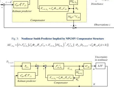
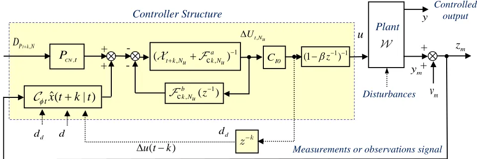
Remarks: The expressions for the NPGMV control (81) and (85) lead to alternative structures for implementation but the second in Fig. 2, is more suitable for implementation. Inspection of the cost term (84) when the input

costing FCN0 is null gives , , ,

0

,N CN N c , N

t k+ P Et P t k+ k NUt

Φ = + and the limiting case of the NPGMV controller is related to an NGMV controller [12].

,

P t k N

D

+

Measured output or observations signal

u

-Controller structure

Disturbances Plant



-m

z

β − −

− 1 1

(1 z ) C_I0

1 ,

ck Nu

−



1 ,_{k Nu}



+

_{t k N}_, u ,

CNt

P

φ +



_tx tˆ( k t| )

+

m

v

m

y

∆ 0 , t Nu

U

0( )

u t k

∆ −

Controlled output

,

t Nu

U

∆

,

d m

d d

y

Fig. 2: Implementation Form of NPGMV State-Dependent Controller Structure

ck