Optimal controller gains for inner current controllers in VSC inverters

OPTIMAL CONTROLLER GAINS FOR INNER CURRENT

CONTROLLERS IN VSC INVERTERS

A.D. Giles*, L. Reguera*, A.J. Roscoe*

*University of Strathclyde, Scotland, alexander.giles@strath.ac.uk, luis.reguera@strath.ac.uk

Keywords: vector control, tuning, inverters.

Abstract

The standard method for controlling an IGBT inverter (or any VSC inverter for that matter) is by vector current control. This control system consists of two cascaded control loops. One possible realisation of the outer controller is to control the DC bus voltage such that no more power is taken off the DC bus than is available. This creates a current reference, which is fed into the inner current controller. The inner current controller then regulates the current passing through the IGBT such that the desired power is dispatched onto the grid. Whilst most research treats the grid connection as a simple RL circuit, there is little consistency on the method by which the gains of the inner current controller are selected. Internal model control, modulus optimum and root locus methods are just a few of the methods used to find the gains. However, it is not clear which of these methods yields the best performance of the inner current controller. This work suggests that tuning on phase margin or manually tuning may not achieve the best results.

1 Introduction

In order to maximise aerodynamic performance, wind turbines operate a variable-speed strategy whereby the rotor speed is varied in order to hold the ratio of the tip-speed of the blades to the free stream wind speed (upstream of the rotor) constant. Consequently, the generator produces a variable frequency signal which cannot be directly exported onto a transmission system and thus requires the use of power electronics. Similarly, wind farms far offshore are expected to be connected via HVDC links in order to minimise losses. Thus, future power systems will have a strong presence of power electronics.

The most commonly implemented control system for inverters is vector current control. Using a phase-locked loop (PLL) to establish the transform for converting the three-phase voltage vector (with balanced components ,

and ) at the point of common coupling (PCC) to a time-independent vector in a rotating reference frame, , active

and reactive power can be controlled independently. This is attributable to the fact that active power, , and reactive power, , are given by equations (1) and (2) respectively:

(1)

(2)

where is the d-component of the voltage vector in the rotating reference frame, is the d-component of the current vector in the rotating reference frame, and is the q-component of the current vector in the rotating reference frame, . Hence, control over enforces control over ,

while control over enforces control over .

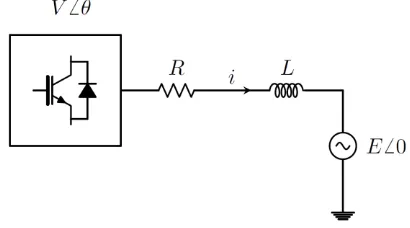
Reference values for and stem from reference values of and . In the case of an inverter, the reference value of is typically obtained from the voltage level on the DC bus in order to avoid a collapse of the DC bus voltage. Due to the Pulse Width Modulation (PWM), an inverter is coupled with filtering equipment to remove harmonic content. An LC filter is typically employed between the inverter and the PCC. For frequency domain analyses, the system which the inverter is connecting to may be modelled as a simple RL circuit as shown in figure 1:

Figure 1: Single-line representation of the connection of an inverter to a grid.

The capacitor dynamics occur at a frequency range which makes the omission of the capacitor from the analysis acceptable. The resistance for power electronics devices will be low (of the order of 0.01pu).

Applying the dq0-transformation is to the dynamic equation of an RL circuit yields the following expression:

( )* + ( ) 2 3(3)

* ( ) + 2

( )

3 (4)

where ( ) is the dq0-transformation matrix established by the PLL and being the phase of :

( ) [ ( ) (

) ( ) ( ) ( ) ( )] (6)

is the three-phase voltage vector at the converter, is

the three-phase voltage vector at the PCC, is the resistance (assumed to be the same for each phase), is the

three-phase current vector and the three-phase reactance (assumed to be the same for each phase).

Let the output of PI controllers regulating and be

, - :

0 1 (7)

The control topology is thus as shown in figure 2:

Figure 2: Control system topology for inner current controller

Coupling equation (5) with equation (7), it follows that

(8)

Taking the Laplace transform yields the open loop transfer function of the RL plant:

( ) ( ), - (9)

where is the complex frequency, . Since the output of the PI controllers is , it also follows that

0

1 , -(10)

Coupling equation (9) with equation (10), the closed-loop transfer function for the inner current controller is then produced:

( )

( )

( ) (11)

where and are the proportional and integral gains respectively. It is also a simple task using equation (9) to obtain the open loop transfer function including the PI controller:

.

/ . / (12)

The derivation of equations (11) and (12) neglects any delays due to the phase-locking of the PLL and other computational delays. According to Kalitjuka computational and switching delays may be accommodated by modifying equation (12) as follows [1]:

.

/ .

/ . / (13)

where is the time delay in the inner current control loop.

Including the delay does still not change the dominant time-constant of the open-loop transfer function, and, by extension, the dominant pole of the system. That is, the dominant time constant, , is

(14)

Analysis of the open-loop and closed-loop transfer functions of a plant allows an engineer to choose what the gains of the control loop should be. Typical control objectives are sufficiently fast response time, small overshoot, acceptable damping etc. A survey of the literature suggests a wide range of tuning techniques are employed, ranging from simple trial-and-error tuning to analytically driven methods such as root locus, internal model control and modulus optimum. However, a comparison between the performance of the controllers with a wide range of different tuning methods is not available. The aim of this paper is to provide insight into what might be the optimal tuning method for the inner current controller.

The structure of this paper is as follows: first a review of four different tuning methods is provided; second, a description of the simulation model is presented; third, results are provided demonstrating the performance of each control system; finally, conclusions and recommendations are presented.

2 Review of tuning algorithms

Four tuning methods are compared: a rule-of-thumb pair of gains based on manual tuning; application of the internal

PI

model control; tuning based on gain and phase margins; and modulus optimum.

2.1 Manual tuning

Of the four tuning methods covered in this text, one is based on experimental performance only, with no theoretical justification. The gains in per-unit form are as follows [2]:

(15) (16)

These gains are rule-of-thumb expressions. The advantage of these expressions is that they have been proven to give stable performance in real-life. On the other hand, one disadvantage is that it is not possible to know where such rule-of-thumb expressions might not be suitable without consulting the transfer functions. There is no guarantee of stability be ensured generally. Upon finding a scenario whereby instability is suggested by the transfer functions, the control engineer then needs to seek an alternative tuning method based on a more theoretical reasoning. Furthermore, it is unlikely that rule-of-thumb gains are optimal.

2.2 Internal Model Control

The application of internal model control (IMC) to inner current controller tuning was elaborately detailed by Harnefors. The key advantage of IMC is that it provides both and when only one desired parameter is specified: the closed-loop bandwidth. Let the desired bandwidth be . Applying the IMC method yields two simple expressions for

and [3]:

(17) (18)

Typically, the bandwidth is limited to no more than 20% of the switching frequency, [3]. For modern IGBT devices, it is possible to achieve values of of 2 kHz [4].

Alternatively, due to the fact that the system is only of the first order, it is possible to define and solely on the rise-time, , using the relation,

(19) i.e.

. / (20) . / (21)

However, since interaction with the inner PWM control system is to be avoided, it is preferable to set the bandwidth by the switching frequency of the converters.

2.3 Tuning on Gain and Phase Margins

A single transfer function is actually two equations: one which corresponds to the Bode magnitude plot, and a second which corresponds to the Bode argument plot. Gain margin (GM) is defined as difference between the magnitude of the system response and 0dB at the frequency at which the phase is -180 degrees. Phase margin (PM) is defined as the difference between the phase and -180 degrees at the crossover frequency (the frequency at which the magnitude in dB is zero). Thus, by setting target gain and phase margins, there is a sufficient number of equations to solve the proportional and integral gains analytically. Alternatively, one could tune based on PM and bandwidth, . This is more sensible as the switching frequency imposes constraints on bandwidth.

Generally, control systems are designed to have 60 degrees of phase margin.

2.4 Modulus Optimum

The control objective of the modulus optimum technique is to maximise the cut-off frequency whilst remaining within the constraints of the system. For the inner current controller, inspection of the open loop transfer function demonstrates that there is one dominant pole. Modulus optimum involves setting the integral time constant of the PI controller to cancel out the dominant pole. The dominant time constant is as given by equation 14.

The gains of the PI controller are then calculated using equations (22) and (23) [1]:

( ) (22)

(23)

where is the cut-off frequency, and is the first order delay of the converter, given as follows [1]:

(24)

Application of the modulus optimum is thus supported by experimental results according to section 2.1.

3 Simulation setup

A simple system was constructed in Simulink (SimPowerSystems) in which an inverter was connected onto a stiff grid, representative of figure 1 but with the inclusion of an AC filter. The control system was the same as that shown in figure 2.

DC bus is treated as ideal; thus, no outer control loops which set the reference current values were necessary. Thus, the performance could purely be attributed to the choice of gains. Consequently, in this setup, it follows that a change in power output (and so a change in ) is simply made by changing (as opposed to been derived from a measurement of the DC bus voltage as would be done in real life).

Typically, the phase reactor has a resistance and inductance of pu and pu [1,3]. For that reason, these values are used in the simulation. The base voltage and power used in the simulation were 195kV and 0.35GVA respectively in accordance with [5].

The inverter itself is modelled using an average value model approach. The main reason for this is the reduction in computational effort compared to using a full-switching model. Incidentally, this does result in a loss of harmonic content which means a simple PLL with little-to-no filtering could be employed.

For each tuning method, a frequency domain analysis was performed, followed by time-domain simulations of performance of the controller following a step-change in the reference currents, and .

4 Results

4.1 Frequency domain analysis

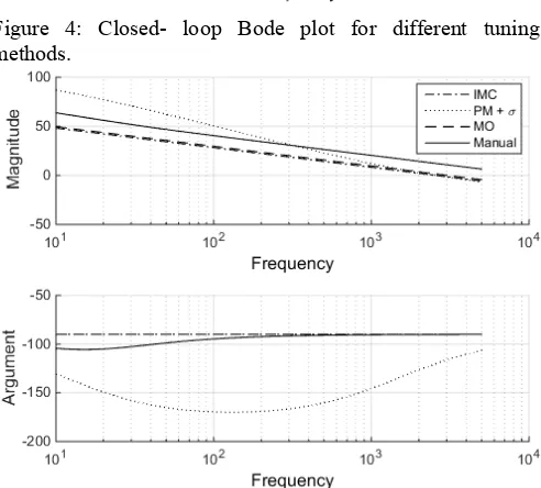
For each tuning method, the performance in the frequency domain could be assessed using equation 11. It is evident from figure 4 that tuning based on gain and phase margins has a stronger response at frequencies above 1kHz than the other tuning methods. This is most likely because the plant naturally has a lot of phase to spare. Thus, in order to yield a phase margin of 60 degrees, the integral gain is large. By consequence, one expects tuning on phase margin can lead to overshoots, which could potentially result in damage to the IGBT components in the inverter.

It is also interesting to note that in all cases, the manual tuning gives higher bandwidth than the other tuning methods. This could potentially lead to problems when using low-switching-frequency devices.

In general, it can be noted that none of the tuning methods gives rise to undesirable resonances and instabilities assuming the resistance and inductance values for pu and pu. Variation in values of are reported in literature. Thus, a sensitivity analysis was conducted to identify any possible problems for any of the tuning methods. Figures 5-8 confirm stability still occurs if pu or pu, which covers the range of inductance values found in literature.

Figure 3: Open-loop Bode plot for different tuning methods.

Figure 4: Closed- loop Bode plot for different tuning methods.

Figure 6: Closed- loop Bode plot for different tuning methods when pu

Figure 7: Open- loop Bode plot for different tuning methods when pu.

Figure 8: Closed- loop Bode plot for different tuning methods when pu.

4.2 Time domain performance

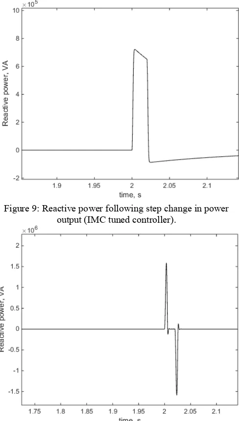
Although vector control in theory provides decoupled control of active and reactive power, it can be seen that irrespective of the control tuning method adopted there is coupling between the two following a step change in one of the reference values such as . This is because a step change in will cause a sudden change in as predicted by equation 5. The control system cannot react instantaneously and thus coupling does occur. However, this level of cross-coupling is small in all cases. It is interesting to note, however, that some tuning algorithms give rise to greater degrees of cross-coupling. The tuning methods which suffers most from this effect is tuning by phase margin.

Figure 9: Reactive power following step change in power output (IMC tuned controller).

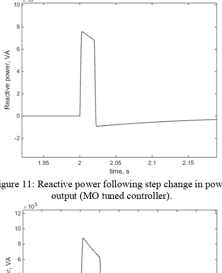
Figure 11: Reactive power following step change in power output (MO tuned controller).

Figure 12: Reactive power following step change in power output (Manually tuned controller).

Focusing purely on the active power response to step changes in , it is observed that irrespective of tuning algorithm, all methods track the requested power output very well.

Figure 11: Active power against time. Step change in active power requested made at s.

IMC and MO tend to give very similar results both in the frequency and time domain. This is understandable when one considers the limit of . Equation (22) simplifies to

. / (25)

If is chosen as , it follows that the proportional gains for both IMC and MO are approximately equivalent, and so consequently the integral gains are also approximately equivalent.

As expected, the tuning method which leads to any overshoots is tuning by phase margin and bandwidth; however, the overshoot does not appear to be significant.

5 Conclusions

IMC and MO are both suitable candidates for tuning the inner current controller and provide a sound theoretical basis for the choice of gains. Manual tuning may be specific to certain ranges of switching frequencies. Tuning based on phase and gain margins does provide the control system designer a higher chance of securing system stability, the primary objective for all control systems. However, the dynamics of the RL system naturally leave a lot of phase margin. Consequently, by setting a phase margin of 60 degrees, the integral gain can end up being large. The drawback of this is that large overshoots can arise which may cause overheating in real-life application. Such a tuning method may therefore require an iterative procedure just to determine what the phase and gain margins should be.

Acknowledgements

This work has been carried out under a grant provided by the EPSRC.

References

[1] T.Kalitjuka, “Control of Voltage Source Converters for Power System Applications” NTNU (2011)

[2] A.J.Roscoe, S.J.Finney, G.M.Burt, “Tradeoffs between AC power quality and DC bus ripple for 3-phase 3-wire inverter-connected devices within microgrids”, IEEE Trans. Power Electronics, volume 26, no. 3, pp. 684-688, (2011). [3] L.Harnefors. H.P.Nee, “Model-based current control of ac drives using the internal model control method,” IEEE Trans. Ind. Appl., vol. 34, no. 1, pp. 133–141, (1998)

[4] B.K.Bose, “Power Electronics and Variable FrequencyDrives”,. New York: IEEE Press, (1997)