City, University of London Institutional Repository
Citation
: Wood, J., Dykes, J., Slingsby, A. and Radburn, R. (2009). Flow trees for
exploring spatial trajectories. Paper presented at the GIS Research UK, 17th Annual Conference, 1 - 3 Apr 2009, University of Durham, Durham, UK.This is the unspecified version of the paper.
This version of the publication may differ from the final published
version.
Permanent repository link:
http://openaccess.city.ac.uk/405/Link to published version
:
Copyright and reuse:
City Research Online aims to make research
outputs of City, University of London available to a wider audience.
Copyright and Moral Rights remain with the author(s) and/or copyright
holders. URLs from City Research Online may be freely distributed and
linked to.
City Research Online: http://openaccess.city.ac.uk/ [email protected]
Flow Trees for Exploring Spatial Trajectories
Jo Wood, Jason Dykes, Aidan Slingsby and Robert Radburn
[image:2.595.74.519.385.521.2]giCentre, School of Informatics, City University London EC1V 0HB Tel.+44 (0)20 7040 0146 Fax +44 (0)20 7040 8584
{jwo | jad7|a.slingsby|sbbd476} @soi.city.ac.uk, www.soi.city.ac.uk/~ {jwo | jad7|sbbb717|sbbd476}
KEYWORDS: trajectories, flows, OD matrices, treemaps, commuting, visualisation
1. Introduction
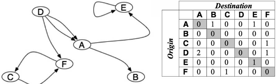
A trajectory is a directed path that defines a link between two spatial locations. That path may be as simple as the Euclidean shortest distance between a start and end point, or may involve a more complex traversal through time and space to travel from start to end. Within GI analysis, trajectories are used to represent phenomena such as movement of people as migration and commuting, goods and information. Trajectories are commonly represented as Origin-Destination Matrices (OD matrices) (Voorhees, 1955) that record the numbers of directed links between a set of start and end points (see Figure 1).
Figure 1. Simple trajectory network and its origin-destination matrix. Note how spatial information is
lost in the matrix view.
This paper presents a novel alternative representation of origin-destination topology that makes it more amenable to the visualization of structure and spatial organisation of trajectories.
2. Challenges for Visualizing Trajectories
Trajectories can be numerous and dense in space making their direct visualization as GIS vector lines problematic. Spatial heterogeneity of density (e.g. commuting flows become denser towards the centre of a city) or constrained flow paths (e.g. along transport networks) can further complicate direct visualisation of all trajectories. While there have been proposals for generalising high density network paths for visualization (e.g. Cui et al 2008), some of the network structure and spatial arrangement can be lost in the process. Rae (2009) explores some of the ways in which the spatial structure of migration trajectories can be preserved using contemporary GI System tools.
origin and destination connections is shown, not the geometry of the paths that connect them. Visualising this matrix as a surface projected in 3-dimensional space, they argued that insight into the topology is gained by clustering OD cells of similar value.
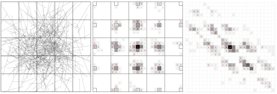
We would argue that there are two significant problems with this approach. Firstly, there seems little benefit in projecting what is a 2-dimensional raster of comparatively low resolution into a 3-dimensional continuous space. This leads to problems of occlusion, dominance of ‘spikes’ and difficulty in navigation and orientation. Secondly, and more significantly, spatial relationships are lost when constructing an OD matrix – 2-dimensional spatial location is collapsed along 1 dimension of each matrix axis. This can result in spurious lineations that are a function of the arbitrary ordering of locations within the matrix (see Figure 2, right).
[image:3.595.72.522.359.512.2]We propose an alternative reordering of the OD matrix, here termed a flow tree, that preserves the spatial arrangement of both origin and destination locations while maintaining the topological structure of the OD matrix. Consider a rectangular space partitioned into n by n grid cells. Each cell represents the origin of trajectories that start within that cell’s bounding box. Next, partition each cell into n by n sub-cells, where each of these smaller child cells represents the location of the destination of any trajectories that originated from their parent cell’s origin location. This is illustrated in Figure 2 where 500 Gaussian random trajectories are partitioned into 5x5 origin cells and then a further 5x5 destination cells inside each origin. This produces a set of 25 small multiples of trajectory destinations, each a copy of the entire region, but filtered and ordered by their origin location. In other words, every origin cell has its own destination map embedded within it.
Figure 2. 500 random trajectories shown as (left) a conventional trajectory map of origin to
destination vectors; (middle) a flow tree; (right) an OD matrix. Numbers of trajectories are indicated as grey shading and numeric symbols. Within the flow tree, locations of trajectories that share the
same origin and destination cell are highlighted.
The flow tree contains the same set of cell values as the OD matrix, but more usefully ordered to show spatial relationships. This can be regarded as a special case of the spatial treemap (Wood and Dykes, 2008a, 2008b) where space is partitioned regularly and the hierarchy is two levels deep. The benefits of the flow tree representation can be seen in Figure 3, which shows 500 random trajectories with significant directional bias. In the conventional trajectory map, this is not visually obvious in the denser central part of the region, but the flow tree shows this clearly, with no destination cells shaded to the east (right) of their origin location.
Figure 3. 500 random trajectories with a west-flowing bias shown as (left) a conventional trajectory map and (right) a flow tree.
[image:4.595.97.489.318.729.2]
3. Partitioning of Space
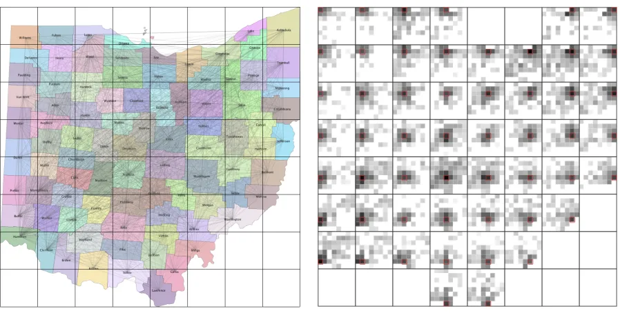
[image:5.595.73.522.165.392.2]The form of the flow tree is dependent partly on the way in which space is partitioned into regions. An important design decision in the flow tree layout is that destination regions are partitioned in exactly the same way as origin regions, thus ensuring the small multiples of the region. To achieve this, the partition must result in self-similar sub-regions that tessellate within their parent region. The simplest of these is to partition into N squares, where N is perfect square.
Figure 5. Square regions for Ohio county-to-county travel to work trajectories and flow tree.
The size of each grid cell should reflect the approximate scale of interest, so for example Figure 5 shows N=64 for Ohio, where each cell is approximately the average size of the counties being examined. However, this can lead to aliasing problems where counties are split between adjacent cells, or inconsistently aggregated within a single cell.
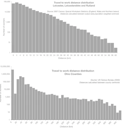
Aggregating at a much coarser scale than the trajectory origin and destination regions can reduce aliasing. For example, Figure 6 shows partition of census output areas (approximately 100 households) into non-square rectangles of 10x8km that reflect the aspect ratio of the entire region.
Figure 6. Rectangular regions used for Leicestershire Output Area travel to work trajectories and
[image:5.595.74.522.549.738.2]Alternatively, if data resolution does not permit aggregation into coarser grid squares, a rectangular spatial treemap tessellation (Wood and Dykes, 2008a) may be applied avoiding arbitrary gridding. Extra ‘dummy nodes’ may have to be inserted into the tree to ensure the number of nodes is a perfect square and thus preserve small multiples (see Figure 7).
Figure 7. Flow tree for Ohio county travel to work using spatial treemap tessellation of counties. 12
extra dummy nodes (white) are added to preserve small multiples of destination cells.
4. Conclusions and Further Work
Visual representation of sets of flows in space is challenging due to localised high density of flows typical in many geographic phenomena. Topological OD matrix views can help to simplify networks, but can also lose important spatial information. The flow trees presented here preserve both topological and spatial structure by using a two-level spatial hierarchy.
hierarchy. We are also exploring how background context mapping can be used to ease the cognition of the spatial transformation involved in projecting a flow tree. Finally, we are investigating non-linear projections to show the spatial heterogeneity of flows in typical urban-rural environments.
Acknowledgements
This work is supported by an ESRC UPTAP User Fellowship RES-163-27-0017 and Leicestershire County Council. Leicestershire travel to work data derived from Census output is Crown copyright and is reproduced with the permission of the Controller of HMSO and the Queen's Printer for Scotland. Output Area boundary data provided through EDINA UKBORDERS with the support of the ESRC and JISC and uses boundary material which is copyright of the Crown.
References
Cui, W., Zhou, H., Qu, H., Wong, P. and Li, X. (2008) Geometry-based edge clustering for graph
visualization. Transactions on Visualization and Computer Graphics, 14(6), 1227-1284.
Marble, D., Gou, Z. and Saunders, J. (1997) Recent advances in the exploratory analysis of
interregional flows in space and time. In Kemp, Z. (ed), Innovations in GIS 4. London: Taylor & Francis, 75-88.
Rae, A. (2009) From spatial interaction data to spatial interaction information? Geovisualisation and
spatial structures of migration from the 2001 UK census. Computers, Environment and Urban Systems, in press DOI:10.1016/j.compenvurbsys.20009.01.007
Voorhees, A. M. (1955) A general theory of traffic movement. Institute of Traffic Engineers Past
Presidents’ Award Paper, New Haven: ITE.
Wood, J. and Dykes, J. (2008a) From slice and dice to hierarchical cartograms: Spatial referencing
of treemaps. In Lambick, D. (ed.) Proceedings of the GIS Research UK 16th National Conference, Manchester Metropolitan University, 1-8.
Wood, J. and Dykes, J. (2008b) Spatially ordered treemaps. IEEE Transactions on Visualization and
Computer Graphics, 14(6) 1348-1355.