Direct computation of scattering matrices for general quantum graphs

City, University of London Institutional Repository

Citation

: Caudrelier, V. and Ragoucy, E. (2010). Direct computation of scattering matrices

for general quantum graphs. Nuclear Physics B, 828(3), pp. 515-535. doi:

10.1016/j.nuclphysb.2009.10.012

This is the published version of the paper.

This version of the publication may differ from the final published

version.

Permanent repository link:

http://openaccess.city.ac.uk/160/

Link to published version

: http://dx.doi.org/10.1016/j.nuclphysb.2009.10.012

Copyright and reuse:

City Research Online aims to make research

outputs of City, University of London available to a wider audience.

Copyright and Moral Rights remain with the author(s) and/or copyright

holders. URLs from City Research Online may be freely distributed and

linked to.

www.elsevier.com/locate/nuclphysb

Direct computation of scattering matrices

for general quantum graphs

V. Caudrelier

_{, E. Ragoucy}

a_{Centre for Mathematical Science, City University London,}

Northampton Square, London, EC1V 0HB, United Kingdom

b_{Laboratoire d’Annecy-le-Vieux de Physique Théorique, LAPTH, CNRS, UMR 5108,}

Université de Savoie, 9 chemin de Bellevue, B.P. 110, F-74941 Annecy-le-Vieux Cedex, France

Received 3 August 2009; accepted 8 October 2009 Available online 13 October 2009

Abstract

We present a direct and simple method for the computation of the total scattering matrix of an arbitrary finite noncompact connected quantum graph given its metric structure and local scattering data at each vertex. The method is inspired by the formalism of Reflection–Transmission algebras and quantum field theory on graphs though the results hold independently of this formalism. It yields a simple and direct algebraic derivation of the formula for the total scattering and has a number of advantages compared to existing recursive methods. The case of loops (or tadpoles) is easily incorporated in our method. This provides an extension of recent similar results obtained in a completely different way in the context of abstract graph theory. It also allows us to discuss briefly the inverse scattering problem in the presence of loops using an explicit example to show that the solution is not unique in general. On top of being conceptually very easy, the computational advantage of the method is illustrated on two examples of “three-dimensional” graphs (tetrahedron and cube) for which other methods are rather heavy or even impractical.

©2009 Elsevier B.V. All rights reserved.

1. Introduction

Excitement in the study of systems on quantum graphs has been revived recently as they pro-vide models for the study of transport properties in quantum wires connected through junctions.

* _{Corresponding author.}

E-mail addresses:[email protected](V. Caudrelier),[email protected](E. Ragoucy). 0550-3213/$ – see front matter ©2009 Elsevier B.V. All rights reserved.

It is largely motivated by the range of different physical applications that can be linked to such models, starting from condensed matter experiments or atomic wires up to chaos and neural networks, for reviews, seee.g.[1,2].

A powerful formalism in this respect is that of quantum fields theory on graphs combined with bosonization techniques. One of the central objects in this approach is the total scattering matrix of the graph and the knowledge of its analytic structure. A number of results are already available in[3–6]but essentially for star graphs. Results that apply to more general graphs can be found in[7–12]where spectral properties of the one-dimensional Laplace operator are studied to obtain general information (and/or construction) of the total scattering matrix. A purely algebraic approach (based on RT algebras[13,14]) for general graphs has been presented in[15], but it uses a rather heavy recursive construction, preventing its possible use for the construction of quantum interacting fields on a graph.

The goal of this paper is to provide an efficient and simple technique to compute this matrix for an arbitrary finite noncompact connected quantum graph knowing only its metric structure and local scattering data at each vertex. The point of view taken here is that the complete graph is obtained by assembling star graphs (single vertex graphs with a certain number of edges) which are well-understood. We obtain an explicit formula for the total scattering matrix. It turns out that our results hold beyond the context of quantum field theory on graphs. Not only do they represent an extension of recent results[10]to the case of graphs with loops but our method also provides a direct (as opposed to recursive[15]) and simple derivation, involving not more than basic linear algebra.

The paper is organised as follows. In Section2we present our formalism to compute directly the scattering matrix associated to a general quantum graph without loop. Once the notation is settled, the calculation is very simple and effective. In the next section, we show how to extend the techniques to graphs with loops. Then, in Section4, we illustrate the techniques in computing the scattering matrix for graphs corresponding to Platonic solids, the cases of tetrahedron and cube being treated in great details. Finally, the last section is devoted to a short conclusion on possible applications.

2. General setting and results

We consider a finite noncompact graph with N vertices that we label with α=1, . . . , N

and with internal and external edges. The graph is compact if it has no external edges. At each vertexαare attached possibly several edges. One can endow the graph with a metric structure: theexternal edgesare associated to infinite half-lines and are connected to a unique vertex; the

internal edgesare associated to intervals of finite length and connect two vertices, possibly not distinct. In the case where an internal edge connects the same vertex, we call it a loop (also called tadpole in the literature). Two edges are adjacent if they are connected by an internal edge. We consider a connected graphi.e. a graph such that for any two verticesα,β there is a sequence

{α1=α, α2, . . . , αq=β}of adjacent vertices. We define an orientation on the edges, and in the

case of internal edges,(αβ)will define an edge with orientation from vertexαto vertexβ. By convention, external edges(α0)are always oriented from the vertex to infinity. On each of these edges, we attachmodes(of fields living on the edge)

aαβ_j (p), j=1, . . . , Nαβ; β=0,1, . . . , N; α=1, . . . , N; α=β,

• α=1,2, . . . , N denotes the vertex to which the edge is attached;

• β=0,1,2, . . . , Ndenotes the vertex linked toαby the edge under consideration, with the convention that external edges corresponds toβ=0;

• j =1, . . . , Nαβnumbers the different edges betweenαandβ,Nαβbeing their total number.

We setNαβ=0 ifαis not connected toβ.

In this way the ordered triplet(α, β, j ) uniquely defines all the oriented edges of the graph. Obviously,(α, β, j )and(β, α, j )define the same edge, but with a different orientation. Hence we have Nαβ=Nβα. We will call internal mode (resp. external mode) a mode living on an

internal edge (resp. external edge).

2.1. General case without loops

For the time being, we assumeNαα=0 for allα=1, . . . , Ni.e. we do not consider loops. We

will see later on that they are easily incorporated in our formalism. The modes are not indepen-dent but are related by two types of fundamental relations defining the scattering and propagation on the graph:

• Local scattering at vertex α: Following the RT-algebra formalism (see e.g. [13,14]), this reads

aαβ_j (p)=

N

γ=0

Nαγ

k=1

sβγ_{α;j k}(p)aαγ_k (−p) ∀j=1, . . . , Nαβ; ∀β=0,1, . . . , N, (2.1)

where sβγ_{α;j k}(p) are the components of the local scattering matrix Sα(p) which satisfies

Sα(p)Sα(−p)=1.

• Propagation on edge(αβj ): As already mentioned, the edges(αβj )and(βαj )are identical (up to the orientation), so that the modesaαβ_j (p)andaβα_j (p)are related. Denoting byd_jαβ= d_jβαthe length of the edge, we have1

aαβ_j (p)=exp−id_jαβpaβα_j (−p). (2.2) The aim now is to obtain the scattering relations directly between the external modesi.e. relations of the form

aα_j0(p)=

N

γ=1

Nγ0

k=1

sαγ_{tot;j k}(p)aγ_k0(−p) ∀j=1, . . . , Nα0; ∀α=1, . . . , N, (2.3)

wheresαγ_{tot;j k}(p)are the components of the total scattering matrix for the graph,Stot(p). This

is most easily achieved by arranging the modes in vectors and using simple linear algebra. De-noteMr×s the vector space of r×s matrices over C. In particular, we identify Mn×n and

End(Cn). We denoteE_i,jr,s ther×smatrix whose only nonzero entry is 1 at position(i, j ). The set{E_ijrs}i=1,...,r;

j=1,...,s

is a basis ofMr×s. We will drop the superscripts every time this does not cause

1 _{The particular form of this relation comes from the fact that we have in mind applications to quantum fields which}

confusioni.e. each time the size of the matrix corresponds to the range of the indices. Similarly, we denote{en_j}j=1,...,nthe canonical basis ofCnand we will use a similar convention. Finally, we

denoteF(p)the space of all (possibly generalized) functions ofp∈C, with the understanding that these functions can be operator-valued in quantum field applications (cf. the modes). The following definitions illustrate our notations and conventions. For a given vertexα, we define different vectors:

• We collect the external modes attached toαin

Aα(p)=

⎛ ⎝

aα₁0(p) .. .

aα_N0

α0(p)

⎞ ⎠₌Nα0

j=1

ej⊗aαj0(p)∈CNα0⊗F(p). (2.4)

• We collect the internal modes attached toαin

Bα(p)=

⎛ ⎜ ⎜ ⎜ ⎜ ⎜ ⎜ ⎜ ⎜ ⎜ ⎜ ⎜ ⎜ ⎜ ⎜ ⎜ ⎜ ⎜ ⎜ ⎜ ⎜ ⎜ ⎜ ⎝

aα₁1(p) .. .

aα_N1

α1(p)

aα₁2(p) .. .

aα_N2

α2(p) .. . .. .

aαN₁ (p) .. .

aαN_N

αN(p) ⎞ ⎟ ⎟ ⎟ ⎟ ⎟ ⎟ ⎟ ⎟ ⎟ ⎟ ⎟ ⎟ ⎟ ⎟ ⎟ ⎟ ⎟ ⎟ ⎟ ⎟ ⎟ ⎟ ⎠ , (2.5)

where only the modes withNαβ=0 appear. For conciseness,2we write this as

Bα(p)= N

β=1

Nαβ

j=1

eβ⊗ej⊗aαβ_j (p)∈Cνα⊗F(p), (2.6)

whereνα=Nβ₌1Nαβis the number of internal edges attached toα. This makes the

follow-ing computations a lot more transparent but the reader should remember the actual content and size of each vector.

• Similarly, we collect all the modes attached toαin

Aα(p)= N

β=0

Nαβ

j=1

eβ+1⊗ej⊗aαβj (p)∈C

Nα⊗F_{(p), (2.7)}

2 _{The explicit, longer formula is} Bα(p)=

qα

p=0

βp+1−1

β=βp+1 Nαβ

j=1

eN_β−−_pqα⊗ej⊗aαβj (p),

where Nα =Nα0+να is the total number of edges attached to α. This way, Aα is the

concatenation ofAα andBα withAα “sitting on top”.

With the same conventions, we introduce

Sα(p)= N

β,γ=0

Nαβ

j=1

Nαγ

k=1

Eβ+1,γ+1⊗Ej k⊗sβγ_{α;j k}(p)∈End

CNα⊗F_{(p), (2.8)}

so the relations(2.1)read

Aα(p)=Sα(p)Aα(−p), ∀α=1, . . . , N. (2.9)

The set of relations(2.9)can be gathered into a single one:

A(p)=S(p)A(−p) withA(p)=

N

α=1

eα⊗Aα(p)andS(p)= N

α=1

Eαα⊗Sα(p).

(2.10) Remark thatA(p)∈CNe+2Ni⊗F_(p)whereN

e=Nα=1Nα0is the total number of external

edges andNi=

1αβNNαβis the total number of internal edges. Then, we introduce

B(p)=

N

α=1

eα⊗Bα(p)∈C2Ni⊗F(p), (2.11)

and

E(p)=

N

α,β=1

Nαβ

j=1

Eα,β⊗Eβ,α⊗Ejj⊗exp

−id_jαβp∈EndC2Ni⊗F_{(p), (2.12)}

so the relations(2.2)read

B(p)=E(p)B(−p). (2.13)

It is easy to see that

E(p)E(−p)=

N

α,β=1

Nαβ

j=1

Eα,α⊗Eβ,β⊗INαβ

that acts as the identity matrix12Ni. The final step is to decompose the matrixS(p)into four

submatrices related to external or internal edges:

S(11)(p)=

N

α=1

Nα0

j,k=1

Eαα⊗Ej k⊗s00α;j k(p)∈End

CNe⊗F_{(p), (2.14)}

S(12)(p)=

N

α,γ=1

Nα0

j=1

Nαγ

k=1

Eαα⊗E1,γ ⊗Ej k⊗s0_αγ_{;j k}(p)∈MNe×2Ni⊗F(p), (2.15)

S(21)(p)=

N

α,β=1

Nαβ

j=1

Nα0

k=1

S(22)(p)=

N

α,β,γ=1

Nαβ

j=1

Nαγ

k=1

Eαα⊗Eβ,γ ⊗Ej k⊗sβγ_{α;j k}(p)∈End

C2Ni⊗F_{(p). (2.17)}

Therefore, the set of all the relations we have becomes

A(p)=S(11)(p)A(−p)+S(12)(p)B(−p), (2.18)

B(p)=S(21)(p)A(−p)+S(22)(p)B(−p), (2.19)

B(p)=E(p)B(−p). (2.20)

Assuming thatE(p)−S(22)(p)is invertible this yields the desired relations in the form

A(p)=Stot(p)A(−p), (2.21)

with

Stot(p)=S(11)(p)+S(12)(p)

E(p)−S(22)(p)−1S(21)(p). (2.22) The internal modes can be expressed in terms of the external ones:

B(p)=E(−p)−S(22)(−p)−1S(21)(−p)A(p). (2.23)

These two formulas are the central result of this work. We note that in the course of our inves-tigation, we discovered that the analog of the result(2.22)has been found in[10]in the setting of abstract graph theory and using the formalism of Grassmann variables. However, the proof is based on the notion of generalized star product [8] and requires a rather involved proof by induction on the size of the graph. Here, it is obtained directly by simple linear algebra and ready to use for computations (either analytical or numerical).

2.2. Discussion

We have checked that our formula reproduces known results obtained by other methods for simple graphs (star-triangle, etc.)[7,8,15]. In the following, we present in detail the computation for new graphs, especially in 3D, for which the previous methods are impractical analytically. Our method presents several advantages compared to previous ones. First, as just mentioned, it is computationally easier and one does not have to worry about the sequence of steps used in iterative methods where one has to make sure that fusing two given vertices and then a third gives the same results a fusing the first and third and then the second (cf.[15]). The only task involved is the inversion of a matrix and there are well-known efficient methods both analytically and numerically. Then, we have an explicit formula which shows the location of the poles ofStot

(on top of the possible ones from the local matrices which are given data in our approach). They are solutions of

detE(p)−S(22)(p)=0. (2.24) This is important as these poles play a fundamental role in the computation of physical quantities like the conductance in quantum systems defined on graphs (see [5,15]). Finally, for quantum systems on compact graphs,i.e. without external edges, the same equation provides the allowed modes on the graph. In this respect,(2.24)is the generalization to an arbitrary compact quantum graph of the quantization equation

for a particle in a box of lengthL. The matrixS(22)(p)accounts here for the one particle scat-tering occurring at the vertices. In the theory of integrable systems, this type of equations is sometimes called Bethe ansatz equations. However, here we emphasize that it is not related to such an ansatz. In condensed matter physics, the information given by this equation together with the dispersion relation of the model provides the basis of band structure analysis.

Scattering matrix of a graph and RT algebras

We would like to comment on the fact that we callStotthe scattering matrix of the graph. This

comes from the terminology one encounters when one takes a graph such as those described in this paper to model quantum wires for instance. In this context, our method gives the matrix which is known to be the scattering matrix in those models. Also, in the context of quantum field theory on graphs, the total scattering matrix that we obtain is precisely the matrix whose elements are the transition amplitudes between asymptotic states. Indeed, using the formalism of quantum field theory, the modesaαβ_j (p), which are used as labels in the previous general setting, acquire the status of Fourier modes of the quantum fields living on the edges of the graph. Together with another set of modes, denoteda†_jαβ(p), they are creation and annihilation operators acting in a Fock space and obeying the RT-algebra relations. This situation has been described and used in detail in[3,4]for star graphs and in[16]for a simple line of edges. Following the latter, we know that relations(2.1) and (2.2) (together with their hermitian conjugates), in the case where the local scattering matrices derive from the self-adjoint extensions of the one-dimensional Laplace operator, ensure that the complex scalar field

φ_jαβ(x, t)= ∞

−∞ dp

2πa

αβ j (p)e

ipx−ip2_t

(2.26)

living on the edge(α, β, j )withx∈ [0, d_jαβ]satisfies the Schrödinger equation3

i∂t+∂x2

φαβ_j (x, t)=0, (2.27)

together with the boundary conditions

N

γ=0

Nαγ

k=1

C_αβγ_{;j k}φαγ_k (0, t )+D_αβγ_{;j k}∂xφkαγ(0, t )

=0, (2.28)

where the matricesCα andDα form the local scattering matrix Sα(p)as explained in [7]. In

this setting, an incoming asymptotic state on thej-th external edge attached to the vertexαis given bya†_jα0(p)withp <0 while an outgoing state corresponds top >0. Hence the scattering amplitude between an incoming and an outgoing state is

0|aβ_j0(−q)a_k†α0(p)|0 , p, q >0, (2.29)

where|0 is the vacuum state annihilated by thea’s (see[13]for more details). The RT alge-bra formalism then enables to compute this scattering amplitude using the following exchange relations between the external (and independent) generators

3 _{This is just an example of governing equation one might want to use on the edges. For a relativistic model, one simply}

a_jα0(p)aβ_k0(q)−a_kβ0(q)aα_j0(p)=0, (2.30)

a_j†α0(p)a†_kβ0(q)−a_k†β0(q)a†_jα0(p)=0, (2.31)

aα_j0(p)a†_kβ0(q)−a†_kβ0(q)aα_j0(p)=2π δj kδαβδ(p−q)+2πsαβtot_;j k(p)δ(p+q), (2.32)

where sαβ_{tot;j k}(p) are the elements of the total scattering matrix Stot(p) obtained in (2.22)

from(2.1) and (2.2). Then one gets

0|aβ_j0(−q)a†_kα0(p)|0 =2πsαβ_{tot;j k}(−q)δ(p−q), p, q >0. (2.33) This also shows that, given the metric and local scattering data of the graph, the total scattering matrix is unique.

2.3. Properties

To be consistent, our general formula should not depend on the numbering of the internal edges or vertices (internal permutation) and should transform appropriately under a permutation of the external modes (external permutation). LetΠ be an external permutation acting onA(p)

andP an internal permutation acting onB(p). It is easy to see that this induces the transforma-tions

S(11)(p)→Π S(11)(p)Π−1, (2.34)

S(12)(p)→Π S(12)(p)P−1, (2.35)

S(21)(p)→P S(21)(p)Π−1, (2.36)

S(22)(p)→P S(22)(p)P−1, (2.37)

E(p)→P E(p)P−1, (2.38)

producingStot→Π StotΠ−1as it should. Therefore, in examples or applications, one can always

fix a convenient numbering of edges and vertices and work up to an external permutation. In view of physical application, we must also be concerned with the properties of Stot. We

have seen already thatSα(p)Sα(−p)=1Nα. This implies

Stot(p)Stot(−p)=1Ne. (2.39)

To see this, note that the block matrix made of(2.14)–(2.17)is related toS(p)given in(2.10)by

S(p)≡

S(11)(p) S(12)(p) S(21)(p) S(22)(p)

=P S(p)P−1, (2.40)

whereP is the permutation matrix defined by

PA(p)=

A(p) B(p)

. (2.41)

Then by direct calculation and upon usingS(p)S(−p)=1Ne+2Ni andE(p)E(−p)=12Ni we

get

Stot(p)Stot(−p)=1Ne+S

(12)_(p)E(p)−S(22)_(p)−1

where

M=12Ni−

E(p)−S(22)(p)E(−p)−S(22)(−p)−E(p)−S(22)(p)S(22)(−p)

−S(22)(p)E(−p)−S(22)(−p)−S(22)(p)S(22)(−p)

=0. (2.43)

Now the local scattering matrices can be required to have additional properties, like unitarity. This is the case in particular if they arise from non-dissipative local boundary conditions emerg-ing from self-adjoint extensions of the free one-dimensional Hamiltonian (seee.g.[7]). One then has unitarity

S_α†(p)=S_α−1(p). (2.44)

Following the same type of argument as above, one finds thatStotis also unitary.

We finish this section by providing a few properties ofE(p). It is symmetric and we have already seen thatE(p)E(−p)=12Ni. In particularE(0)

2₌₁

2Ni so its eigenvalues are±1 and

are equally degenerate. Also,E(0)is a permutation matrix andE(p)is a generalized permutation matrix (with coefficients of the typee−ipd

αβ

j _{) which can be written as a product of a permutation}

matrix and a diagonal matrix

E(p)=D(p)E(0)=E(0)D(p), (2.45)

where

D(p)=

N

α,β=1

Nαβ

j=1

Eα,α⊗Eβ,β⊗Ejj⊗exp

−id_jαβp, (2.46)

with

D(p)D(q)=D(p+q), p, q∈C. (2.47)

3. Including loops

The case of loops attached to single vertices can be treated with minor modifications in our formalism. Essentially, the idea is again to see a loop attached to a given vertex αas arising from the gluing of two edges attached to this vertex. This will be most easily incorporated in the general formalism if we use the following trick for notations. LetNαα=0 be the number

of loops attached to vertexα. To each loopj,j =1, . . . , Nααcorrespond two modes4aαα_2j−1(p)

andaαα_2j(p)which are related by

a₂αα_j−1(p)=e−ipdjαα_aαα

2j(−p), j =1, . . . , Nαα. (3.1)

We collect these modes in two-component vectors

aαα_j (p)=

a₂αα_j−1(p) a₂αα_j(p)

, j=1, . . . , Nαα. (3.2)

We denote all the components of the local scattering matrixSα(p)related to the loop modes

bys_ααβ_{;j k}(p),j=1, . . . ,2Nαα,k=1, . . . , Nαβ;sβα_{α;j k}(p),j =1, . . . , Nαβ,k=1, . . . ,2Nαα; and

s_ααα_{;j k}(p),j, k=1, . . . ,2Nαα. Mimicking(3.2), we then define, forα=β,

sαβ_{α;j k}(p)=

sαβ_α;2j−1,k(p) s_ααβ_;2j,k(p)

, j =1, . . . , Nαα, k=1, . . . , Nαβ, (3.3)

sβα_{α;j k}(p)=( s_αβα_;j,2k−1(p) s_αβα_;j,2k(p) ) , j=1, . . . , Nαβ, k=1, . . . , Nαα, (3.4)

and also,

sαα_{α;j k}(p)=

_sαα

α;2j−1,2k−1(p) s

αα

α;2j−1,2k(p)

s_ααα_;2j,2k−1(p) s_ααα_;2j,2k(p)

, j, k=1, . . . , Nαα. (3.5)

Finally, we define

eαβ_j (p)=

eipd αβ

j _{, ifβ}=_αandN

αβ=0,

eipdααj 0 1

1 0

, ifβ=αandNαα=0.

(3.6)

With all this, the relations defining scattering and propagation on the graph take the same form as before (cf.(2.1) and (2.2))

aαβ_j (p)=

N

γ=0

Nαγ

k=1

sβγ_{α;j k}(p)aαγ_k (−p) ∀j =1, . . . , Nαβ; ∀β=0,1, . . . , N (3.7)

and

aαβ_j (p)=e_jαβ(−p)aβα_j (−p) ∀j=1, . . . , Nαβ; ∀β=0,1, . . . , N. (3.8)

Therefore, all the formalism and the results developed in Section2.1hold in the same form, pro-vided one substituteseαβ_j (−p)fore−ipd

αβ

j _{in(2.12). One should not be deceived by the apparent}

similarity of the results with or without loops. In general, the consequences of adding a loop in a given graph can be drastic.

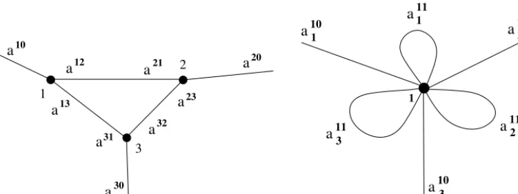
However, as the formalism suggests, allowing for loops in graphs opens the possibility that two topologically completely different graphs can have exactly the same total scattering matrix. This is illustrated on the example below. In particular, this shows that the uniqueness of the inverse scattering problem, as discussed in[9], does not extend to the case of graphs with loops.5 The equivalent statement in terms of the Schrödinger operator on a graph was discussed in[17]

where it was shown that in general the knowledge of the scattering matrix of a noncompact graph is not enough to fix its topological structure and the boundary conditions at the vertices.

We consider the two graphs depicted inFig. 1below. To illustrate our notations, we have displayed the modes involved in the construction, dropping thep-dependence for conciseness. They are topologically completely different, one being a triangle with one external edge attached to each vertex and the other being a single vertex star graph with three external edges and three loops attached to it. Note that for the triangle, we drop the unnecessary Latin subscripts since

Nαβ=1 for allα=1,2,3 andβ=0,1,2,3,β=α.

We assume that the scattering and propagation data is given as follows (we drop again thep

dependence for clarity),

5 _{Uniqueness is only guaranteed if one requires in addition that the number of vertices is maximal (cf. Theorem 4.6}

Fig. 1. Two topologically different graphs with the same total scattering matrix. Left: triangle. Right: star graph with loops.

For the triangle,

S1=

⎛ ⎜ ⎝

s00₁ s02₁ s03₁ s20₁ s22₁ s23₁ s30₁ s32₁ s33₁

⎞ ⎟

⎠, S2=

⎛ ⎜ ⎝

s00₂ s01₂ s03₂ s10₂ s11₂ s13₂ s30₂ s31₂ s33₂

⎞ ⎟

⎠, S3=

⎛ ⎜ ⎝

s00₃ s01₃ s02₃ s10₃ s11₃ s12₃ s20₃ s21₃ s22₃

⎞ ⎟ ⎠,

(3.9)

giving the four blocks as defined in(2.14)–(2.17)in the form

S(11)=

⎛ ⎝s

00

1 0 0

0 s00₂ 0 0 0 s00₃

⎞

⎠, S(22)=

⎛ ⎜ ⎜ ⎜ ⎜ ⎜ ⎜ ⎜ ⎜ ⎜ ⎝

s22₁ s23₁ 0 0 0 0

s32₁ s33₁ 0 0 0 0 0 0 s11₂ s13₂ 0 0 0 0 s31₂ s33₂ 0 0 0 0 0 0 s11₃ s12₃

0 0 0 0 s21₃ s22₃

⎞ ⎟ ⎟ ⎟ ⎟ ⎟ ⎟ ⎟ ⎟ ⎟ ⎠ , (3.10)

S(12)=

⎛ ⎝s

02 1 s

03

1 0 0 0 0

0 0 s01₂ s03₂ 0 0 0 0 0 0 s01₃ s02₃

⎞

⎠, S(21)=

⎛ ⎜ ⎜ ⎜ ⎜ ⎜ ⎜ ⎜ ⎝

s20₁ 0 0

s30₁ 0 0 0 s10₂ 0 0 s30₂ 0 0 0 s10₃

0 0 s20₃

⎞ ⎟ ⎟ ⎟ ⎟ ⎟ ⎟ ⎟ ⎠ , (3.11) and

Et =

⎛ ⎜ ⎜ ⎜ ⎜ ⎜ ⎝

0 0 e−ipd12 0 0 0 0 0 0 0 e−ipd13 0

e−ipd12 0 0 0 0 0

0 0 0 0 0 e−ipd23

0 e−ipd13 0 0 0 0 0 0 0 e−ipd23 _{0 0}

For the star graph, T = ⎛ ⎜ ⎜ ⎜ ⎜ ⎜ ⎜ ⎜ ⎜ ⎜ ⎜ ⎝

t00_1;11 0 0 t01_1;11 t01_1;12 t01_1;13

0 t00_1;22 0 t01_1;21 t01_1;22 t01_1;23

0 0 t00_1;33 t01_1;31 t01_1;32 t01_1;33 t10_1;11 t10_1;12 t10_1;13 t11_1;11 t11_1;12 t11_1;13 t10_1;21 t10_1;22 t10_1;23 t11_1;21 t11_1;22 t11_1;23 t10_1;31 t10_1;32 t10_1;33 t11_1;31 t11_1;32 t11_1;33

⎞ ⎟ ⎟ ⎟ ⎟ ⎟ ⎟ ⎟ ⎟ ⎟ ⎟ ⎠ ≡

T(11) T(12) T(21) T(22)

, (3.13)

and

Es=

⎛ ⎜ ⎜ ⎜ ⎜ ⎜ ⎝

0 e−ipd111 0 0 0 0

e−ipd111 _{0 0 0 0 0}

0 0 0 e−ipd211 _{0 0}

0 0 e−ipd211 _{0 0 0}

0 0 0 0 0 e−ipd311

0 0 0 0 e−ipd311 ₀

⎞ ⎟ ⎟ ⎟ ⎟ ⎟ ⎠ . (3.14)

The lengths of the internal edges of the triangle are related to the lengths of the loop in the star graph by

d12=d₁11, d23=d₃11, d23=d₂11, (3.15) and the following relations for the scattering data hold, showing in particular the matrix structure defined in(3.3)–(3.5)in the case of loops,

t00_1;11=s00₁ , t00_1;22=s00₂ , t00_1;33=s00₃ , (3.16)

t01_1;11=(s02₁ 0) , t01_1;12=(0 0) , t01_1;13=(s03₁ 0) , (3.17)

t01_1;21=(0 s01₂ ) , t01_1;22=(s03₂ 0) , t₁01_;23=(0 0) , (3.18)

t01_1;31=(0 0) , t01_1;32=(0 s02₃ ) , t01_1;33=(0 s01₃ ) , (3.19)

t10_1;11=

s20₁

0

, t10_1;12=

0

s10₂

, t10_1;13=

0 0

, (3.20)

t10_1;21=

0 0

, t10_1;22=

s30₂

0

, t10_1;23=

0

s20₃

, (3.21)

t10_1;31=

s30₁

0

, t10_1;32=

0 0

, t10_1;33=

0

s10₃

, (3.22)

t11_1;11=

s22₁ 0 0 s11₂

, t11_1;12=

0 0

s13₂ 0

, t11_1;13=

s23₁ 0 0 0

, (3.23)

t11_1;21=

0 s31₂

0 0

, t11_1;22=

s33₂ 0 0 s22₃

, t11_1;23=

0 0 0 s21₃

, (3.24)

t11_1;31=

s32₁ 0 0 0

, t11_1;32=

0 0 0 s12₃

, t11_1;33=

s33₁ 0 0 s11₃

The fact that these two graphs give rise to the same total scattering matrix follows from the fact that their scattering data are related by an internal permutation

P=

⎛ ⎜ ⎜ ⎜ ⎜ ⎜ ⎝

1 0 0 0 0 0 0 0 1 0 0 0 0 0 0 1 0 0 0 0 0 0 0 1 0 1 0 0 0 0 0 0 0 0 1 0

⎞ ⎟ ⎟ ⎟ ⎟ ⎟ ⎠

, (3.26)

such that

P S(22)P−1=T(22), P EtP−1=Es,

S(12)P−1=T(12), P S(21)=T(21). (3.27) Then,

Stottriangle=S(11)+S(12)

Et−S(22)

₋1

S(21)

=S(11)+S(12)P−1P EtP−1−P S(22)P−1

₋1

P S(21)

=T(11)+T(12)Es−T(22)

₋1

T(21)

=S_totstar. (3.28)

4. Platonic solids

In this section, we illustrate the freedom on numbering and the use of formula (2.22) on the convex regular polyhedra known as Platonic solids (tetrahedron, cube, octahedron, dodeca-hedron, icosahedron)[18]. Once the scattering matrix is known, physical quantities associated to the graph can easily be computed, such as the conductance, using the formalism developed in[3]. The calculation essentially relies on the pole structure and the general techniques have been explicited in[15].

We carry out explicit calculations in the case of the tetrahedron and the cube. This choice is primarily motivated by aesthetic and academic criteria rather than any particular practical application. It also shows the computational advantage of our method over recursive ones on rather involved graphs. More precisely, we consider graphs whose internal edges and vertices correspond to Platonic solids and for which exactly one external edge is attached to each vertex. This corresponds toNαβ=1, α=1, . . . , N,β=0, . . . , N,α=β. Note that the condition of

regularity yieldsd₁αβ≡dfor allα, β=1, . . . , N. Also, all the vertices are connected to the same number of vertices soνα ≡ν is the same for allα=1, . . . , N.N is even for all those graphs.

Finally, from the general theory of graph colouring, seee.g.[19], it is known that we can assign a label (or colour)a∈ {1, . . . , ν}to the edges connected to the same vertex in a way compatible with the graph,i.e. in colour terms, such that no two edges connected to the same vertex have the same colour and each edge can only have one colour. This allows us to define functionsnα,

α∈ {1, . . . , N}from{1, . . . , ν}to{1, . . . , N}such thatnα(a)=β if and only ifβ is connected

toαby the edge labelleda. We use the conventiona=0 for external edges and setnα(0)=0

for allα∈ {1, . . . , N}. By construction, we have the following properties

nα(a)=β⇔nβ(a)=α, nα(a)=nβ(a)⇔α=β,

In view of formula(2.22), the main object of interest isE(p)−S(22)(p)which we seek to invert. With our notations, we get

E(p)=e−ipd

N

α=1

ν

a=1

Eα,nα(a)⊗Eaa,

S(22)(p)=

N

α=1

ν

a,b=1

Eα,α⊗Eab⊗sabα (p), (4.2)

where the local matrices read

Sα(p)= ν

a,b=0

Ea+1,b+1⊗sabα (p), α=1, . . . , N. (4.3)

For later convenience, we define a reduced scattering matrix containing only the information about scattering on the internal edges

S_αred(p)=

ν

a,b=1

Ea,b⊗sabα (p), α=1, . . . , N. (4.4)

Let us also define

Ea= N

α=1

Eα,nα(a). (4.5)

ThenE(p)=e−ipdν_a=1Ea⊗Eaaand from the general properties ofE(or by direct

calcula-tion) we find

Ea=Eat =Ea−1, a=1, . . . , ν. (4.6)

ThereforeEais diagonalizable with eigenvalues±1 each degenerateN₂ times and with

eigenvec-torsv_α=√1

2(eα+enα(a)),= ±1,α < nα(a), forming an orthonormal basis.

4.1. Tetrahedron

For the tetrahedron,N=4,ν=3 and the matricesEaenjoy the additional property

EaEb=EbEa, ∀a, b=1,2,3, (4.7)

due to the fact that

∀β∈ {1,2,3,4},∀a, b∈ {1,2,3}, nnβ(a)(b)=nnβ(b)(a). (4.8)

This can be seen to hold by direct inspection on Fig. 2and holds also for other inequivalent numberings.

From (4.7), they can be diagonalized simultaneously. As already explained, to fix ideas we can fix a numbering without loss of generality since we work up to permutations. In the present case, changing the edges and or vertices numbering amounts to interchanging theEa’s. From the

figure we obtain

E1=

⎛ ⎜ ⎝

0 0 0 1 0 0 1 0 0 1 0 0 1 0 0 0

⎞ ⎟

⎠, E2=

⎛ ⎜ ⎝

0 1 0 0 1 0 0 0 0 0 0 1 0 0 1 0

⎞ ⎟

⎠, E3=

⎛ ⎜ ⎝

0 0 1 0 0 0 0 1 1 0 0 0 0 1 0 0

⎞ ⎟

Fig. 2. Tetrahedron with an example of numbering.

and a diagonalizing matrix is

T =1

2

⎛ ⎜ ⎝

−1 1 −1 1 1 −1 −1 1

−1 −1 1 1 1 1 1 1

⎞ ⎟

⎠=T−1=Tt. (4.10) So far, we haven’t taken advantage of the geometry and its symmetries. The scattering can still be different from vertex to vertex (as labelled by the indexαon the local matrices) and at a given vertex, the scattering from edgeato edgebneeds not be the same as the scattering from edgea

to edgecsay. Clearly, this does not respect the natural symmetry of the underlying graph. One can impose that the local scattering matrices be the same for all verticesi.e.Sα(p)≡S(p)and

in particularS_αred(p)≡Sred(p)for allα=1,2,3,4. This already greatly simplifies the problem of inversion. Letτ=T ⊗13andDa=TEaT−1then

τE(p)−S(22)(p)τ−1=e−ipd

3

a=1

Da⊗Eaa−14⊗Sred(p). (4.11)

The matrix on the right-hand side is a block diagonal matrix made of four 3×3 blocks essentially determined bySred

τE(p)−S(22)(p)τ−1=

4

α=1

Eαα⊗

e−ipdIα−Sred(p)

, (4.12)

with

I1=

_{−1 0 0}

0 −1 0 0 0 1

, I2=

_{1 0 0}

0 −1 0 0 0 −1

,

I3=

_{−1 0 0}

0 1 0 0 0 −1

, I4=13. (4.13)

Thus, the problem is reduced to inverting 3×3 matrices. In particular, the poles of Stot are

solutions of

dete−ipdIα−Sred(p)

=0, α=1,2,3,4. (4.14) We now turn to the explicit calculation ofStot in the case where the vertices are described by

our case, each local matrix is the same 4×4 scale invariant matrix whose explicit form has been classified in[3]. Note also that we can take further advantage of the symmetries of the underlying geometry here by imposing for instance that the scattering be invariant under a rotation ofπ/3 around the axis passing through a vertex and the centre of the opposite face. Physically, this means that an incoming particle from the external edge of a vertex has the same probability of being transmitted to any one of the internal edges attached to this vertex. Mathematically, this amounts to requiring thatSsatisfies

1 0 0 J S 1 0 0 J−1

=S, (4.15)

where

J=

_{0 1 0}

0 0 1 1 0 0

, J3=13. (4.16)

Putting everything together, we find two possible local scattering matrices

S1=

⎛ ⎜ ⎜ ⎜ ⎝ −1 2 1 2 1 2 1 2 1 2 − 1 2 1 2 1 2 1 2 1 2 − 1 2 1 2 1 2 1 2 1 2 − 1 2 ⎞ ⎟ ⎟ ⎟

⎠, S2=

⎛ ⎜ ⎜ ⎜ ⎝ −1 2 1 2 1 2 1 2 1 2 5 6 − 1 6 − 1 6 1 2 − 1 6 5 6 − 1 6 1 2 − 1 6 − 1 6 5 6 ⎞ ⎟ ⎟ ⎟

⎠. (4.17)

In the first case, we computeStot(p)as

S_tot1 (p)= 1 G1(p)

−2e−3ipd+e−ipd−114+e−ipd

e−ipd+1A, (4.18) whereG1(p)=(2e−2ipd+e−ipd+1)(2e−ipd−1)and

A=

⎛ ⎜ ⎝

0 1 1 1 1 0 1 1 1 1 0 1 1 1 1 0

⎞ ⎟

⎠. (4.19)

The poles of this matrix are given by

e−ipd=x withx∈

1 2,

−1+i√7 4 ,

−1−i√7 4

. (4.20)

In the second case, we obtain

S_tot2 (p)= 1 G2(p)

−2−6e−3ipd+4e−2ipd+10e−ipd−614

+3e−ipde−ipd−1A, (4.21) whereG2(p)=(6e−2ipd−e−ipd−3)(2e−ipd−1), leading to the poles

e−ipd=x withx∈

1 2,

1+√73 12 ,

1−√73 12

Fig. 3. Cube with an example of numbering.

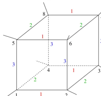
4.2. Cube

For the cube,N=8 andν=3 and the matrices Ea also commute. So one can perform the

same analysis as before.

Based onFig. 3, we get explicitly

E1=

⎛ ⎜ ⎜ ⎜ ⎜ ⎜ ⎜ ⎜ ⎜ ⎜ ⎝

0 1 0 0 0 0 0 0 1 0 0 0 0 0 0 0 0 0 0 1 0 0 0 0 0 0 1 0 0 0 0 0 0 0 0 0 0 1 0 0 0 0 0 0 1 0 0 0 0 0 0 0 0 0 0 1 0 0 0 0 0 0 1 0

⎞ ⎟ ⎟ ⎟ ⎟ ⎟ ⎟ ⎟ ⎟ ⎟ ⎠

, E2=

⎛ ⎜ ⎜ ⎜ ⎜ ⎜ ⎜ ⎜ ⎜ ⎜ ⎝

0 0 0 1 0 0 0 0 0 0 1 0 0 0 0 0 0 1 0 0 0 0 0 0 1 0 0 0 0 0 0 0 0 0 0 0 0 0 0 1 0 0 0 0 0 0 1 0 0 0 0 0 0 1 0 0 0 0 0 0 1 0 0 0

⎞ ⎟ ⎟ ⎟ ⎟ ⎟ ⎟ ⎟ ⎟ ⎟ ⎠ , (4.23)

E3=

⎛ ⎜ ⎜ ⎜ ⎜ ⎜ ⎜ ⎜ ⎜ ⎜ ⎝

0 0 0 0 1 0 0 0 0 0 0 0 0 1 0 0 0 0 0 0 0 0 1 0 0 0 0 0 0 0 0 1 1 0 0 0 0 0 0 0 0 1 0 0 0 0 0 0 0 0 1 0 0 0 0 0 0 0 0 1 0 0 0 0

⎞ ⎟ ⎟ ⎟ ⎟ ⎟ ⎟ ⎟ ⎟ ⎟ ⎠ , (4.24)

and a diagonalizing matrix is

V = 1

2√2

⎛ ⎜ ⎜ ⎜ ⎜ ⎜ ⎜ ⎜ ⎜ ⎜ ⎝

1 −1 1 −1 −1 1 −1 1 1 1 −1 −1 −1 −1 1 1

−1 1 1 −1 1 −1 −1 1

−1 −1 −1 −1 1 1 1 1

−1 1 −1 1 −1 1 −1 1

−1 −1 1 1 −1 −1 1 1 1 −1 −1 1 1 −1 −1 1 1 1 1 1 1 1 1 1

⎞ ⎟ ⎟ ⎟ ⎟ ⎟ ⎟ ⎟ ⎟ ⎟ ⎠

Again assuming that the local scattering matrices are the same at all vertices, we get

VE(p)−S(22)(p)V−1=e−ipd

3

a=1

a⊗Eaa−18⊗Sred(p), (4.26)

where a=VEaV−1 andV =V ⊗13. This is a block diagonal matrix and the problem is

reduced to inverting 3×3 matrices,

E(p)−S(22)(p)−1=V−1

₈

α=1

Eαα⊗

e−ipdIα−Sred(p)

₋1

V, (4.27)

where

I1=13, I2=

_{−1 0 0}

0 1 0 0 0 1

,

I3=

_{1 0 0}

0 −1 0 0 0 1

, I4=

_{−1 0 0}

0 −1 0 0 0 1

, (4.28)

I5=

_{1 0 0}

0 1 0 0 0 −1

, I6=

_{−1 0 0}

0 1 0 0 0 −1

,

I7=

_{1 0 0}

0 −1 0 0 0 1

, I8= −13. (4.29)

We turn to the explicit computation of the total scattering matrix in the two cases(4.17) describ-ing scale and rotation invariant local scatterdescrib-ing at the vertices. In both cases, we find the followdescrib-ing structures forStot: it is a linear combination of matrices in the Abelian group generated by the E’s with coefficients being polynomials ine−ipd. Forj=1,2,

Stotj (p)=a

j

0(p)18+a

j

1(p)E1+a

j

2(p)E2+a

j

3(p)E3+a

j

4(p)E1E2+a

j

5(p)E1E3

+a₆j(p)E2E3+a7j(p)E1E2E3. (4.30)

In the first case, we find

a₀1(p)=8+e

−ipd_−8e−2ipd_−5e−3ipd_−40e−4ipd_+4e−5ipd_−32e−6ipd

4(−1+e−2ipd_+8e−4ipd_+16e−6ipd₎ , (4.31)

a₁1(p)= −5e

−ipd_+e−3ipd_−20e−5ipd

4(−1+e−2ipd_+8e−4ipd_+16e−6ipd₎, (4.32)

a₂1(p)= 3e −ipd

4−16e−2ipd, (4.33)

a₃1(p)= 3e −ipd

4−16e−2ipd, (4.34)

a₄1(p)= − e

−ipd_(1−9e−ipd_+2e−2ipd₎

4(−1+e−ipd_+2e−2ipd_−4e−3ipd_+8e−4ipd₎, (4.35)

a₅1(p)= − e

−ipd_(1−9e−ipd_+2e−2ipd₎

a₆1(p)= e

−ipd_(1+9e−ipd_+2e−2ipd₎

4(−1−e−ipd_+2e−2ipd_+4e−3ipd_+8e−4ipd₎, (4.37)

a₇1(p)= − e

−ipd_+19e−3ipd_+4e−5ipd

4(−1+e−2ipd_+8e−4ipd_+16e−6ipd₎. (4.38)

The poles of the scattering matrix can be then computed. They are given by

e−ipd=x withx∈

±1

2,±

1+i√7 4 ,±

1−i√7 4

. (4.39)

In the second case, we find

a₀2(p)=72+9e

−ipd_−440e−2ipd_−45e−3ipd_+728e−4ipd_+36e−5ipd_−288e−6ipd

4(−9+73e−2ipd_−184e−4ipd_+144e−6ipd₎ ,

(4.40)

a₁2(p)= − 3e

−ipd_(15−67e−2ipd_+60e−4ipd₎

4(−9+73e−2ipd_−184e−4ipd_+144e−6ipd₎, (4.41)

a₂2(p)= 3e −ipd

4−16e−2ipd, (4.42)

a₃2(p)= 3e −ipd

4−16e−2ipd, (4.43)

a₄2(p)= − 3e

−ipd_(−1+3e−ipd_+2e−2ipd₎

4(3−e−ipd_−18e−2ipd_+4e−3ipd_+24e−4ipd₎, (4.44)

a₅2(p)= − 3e

−ipd_(−1+3e−ipd_+2e−2ipd₎

4(3−e−ipd_−18e−2ipd_+4e−3ipd_+24e−4ipd₎, (4.45)

a₆2(p)= 3e

−ipd_(−1−3e−ipd_+2e−2ipd₎

4(3+e−ipd_−18e−2ipd_−4e−3ipd_+24e−4ipd₎, (4.46)

a₇2(p)= 3e

−ipd_(3−7e−2ipd_+12e−4ipd₎

4(9−73e−2ipd_+184e−4ipd_−144e−6ipd₎. (4.47)

The poles of the scattering matrix are given by

e−ipd=x withx∈

±1

2,±

1+√73 12 ,±

1−√73 12

. (4.48)

5. Conclusion and outlooks

We want to stress that in the present paper, themodesas we called them, appear more as con-venient labels than true quantum field theoretic objects. This has two consequences. First, our results are ready to use for applications in quantum field theory on graphs by simply promoting the modes to generators of the RT-algebra [13], as briefly discussed in Section2.2. Second, it means that our results hold in complete generality for abstract graphs with or without loops. In this respect, the present results provide an extension of the results in [10] to the case of loops.6

Finally, this paper lays the ground to applications to transport problems on arbitrary graphs in the spirit of the studies performed ine.g.[3–6]using quantum field theory and bozonization techniques. Indeed, it provides one with the central ingredient which is the total scattering matrix together with its pole structure. Once this structure is known, the calculation of physical data such as the conductance between external edges is rather direct, see e.g.[15]. We will return to these questions in the near future. Let us note that some of them have been addressed in the first quantization approach, where the scattering matrix was computed for continuous wave functions[20], and then used to compute local conserved quantities[21].

References

[1] P. Exner, Leaky Quantum graphs: A review, Proc. Sympos. Pure Math. 77 (2008) 523, arXiv:0710.5903. [2] P. Kuchment, Quantum graphs: An introduction and a brief survey, Proc. Sympos. Pure Math. 77 (2008) 291,

arXiv:0802.3442.

[3] B. Bellazzini, M. Mintchev, P. Sorba, Bosonization and scale invariance on quantum wires, J. Phys. A 40 (2007) 2485, hep-th/0611090.

[4] B. Bellazzini, M. Burrello, M. Mintchev, P. Sorba, Quantum field theory on star graphs, Proc. Sympos. Pure Math. 77 (2008) 639, arXiv:0801.2852.

[5] B. Bellazzini, M. Mintchev, P. Sorba, Boundary bound state effects in quantum wires, arXiv:0810.3101.

[6] B. Bellazzini, M. Mintchev, P. Sorba, Quantum wire junctions breaking time reversal invariance, arXiv:0907.4221. [7] V. Kostrykin, R. Schrader, Kirchhoff’s rule for quantum wires, J. Phys. A 32 (1999) 595–630, math-ph/9806013. [8] V. Kostrykin, R. Schrader, The generalized star product and the factorization of scattering matrices on graphs,

J. Math. Phys. 42 (2001) 1563, math-ph/0008022.

[9] V. Kostrykin, R. Schrader, The inverse scattering problem for metric graphs and the traveling salesman problem, math-ph/0603010.

[10] Sh. Khachatryan, R. Schrader, A. Sedrakyan, Grassmann–Gaussian integrals and generalized star products, J. Phys. A 42 (2009) 304019, arXiv:0904.2683.

[11] Sh. Khachatryan, A. Sedrakyan, P. Sorba, Network models: Action formulation, arXiv:0904.2688. [12] R. Schrader, Finite propagation speed and causal free quantum fields on networks, arXiv:0907.1522.

[13] M. Mintchev, E. Ragoucy, P. Sorba, Scattering in the presence of a reflecting and transmitting impurity, Phys. Lett. B 547 (2002) 313, hep-th/0209052;

M. Mintchev, E. Ragoucy, P. Sorba, Reflection–transmission algebras, J. Phys. A 36 (2003) 10407, hep-th/0303187. [14] V. Caudrelier, M. Mintchev, E. Ragoucy, P. Sorba, Reflection–transmission quantum Yang–Baxter equations,

J. Phys. A 38 (2005) 3431, hep-th/0412159.

[15] E. Ragoucy, Quantum field theory on quantum graphs and application to their conductance, J. Phys. A 42 (2009) 295205, arXiv:0901.2431.

[16] M. Mintchev, E. Ragoucy, Algebraic approach to multiple defects on the line and application to Casimir force, J. Phys. A 40 (2007) 9515, arXiv:0705.1322.

[17] P. Kurasov, F. Stenberg, On the inverse scattering problem on branching graphs, J. Phys. A 35 (2002) 101. [18] Pythagoras, autos ephe,∼500 B.C.;

Theaetetus, Book X of Euclid’s Elements, 300 B.C.

6 _{The more general case where relations(2.2)are replaced by a general invertible connecting matrix is easily}

[19] C. Shannon, A theorem on coloring the lines of a network, J. Math. Phys. 28 (1949) 148–151; V.G. Vizing, On an estimate of the chromatic class of ap-graph, Diskretn. Anal. 3 (1964) 25–30; V.G. Vizing, Critical graphs with given chromatic class, Metody Diskretn. Anal. 5 (1965) 9–17;

P. Erdös, R. Wilson, Note on the chromatic index of almost all graphs, J. Combin. Theory B 23 (1977) 255–257. [20] C. Texier, G. Montambaux, Scattering theory on graphs, J. Phys. A 34 (2001) 10307–10326.

[21] C. Texier, M. Büttiker, Local Friedel sum rule in graphs, Phys. Rev. B 67 (2003) 245410;