Semantic Analysis of Facial Gestures from Video Using a Bayesian Framework

Rochester Institute of Technology

RIT Scholar Works

Theses Thesis/Dissertation Collections

7-19-2011

Semantic Analysis of Facial Gestures from Video

Using a Bayesian Framework

Gati Vashi

Follow this and additional works at:http://scholarworks.rit.edu/theses

Recommended Citation

Semantic Analysis of Facial Gestures from Video Using a

Bayesian Framework

Gati Vashi

[email protected]

http:/ /www.cs.rit.edu/-gdv7368

This M.S. Thesis is submitted to the faculty of the Department of Computer Science, in partial fulfillment of the requirements for the degree of Master of Computer

Science in the Golisano College of Computing and Information Science

Rochester Institute of Technology Rochester, New York

July 19, 2011

Approved by: _ _ __ _ _ _ __ _ _ _ _ _ _ _ _ _ Dr. Roxanne Canosa, Thegis Advisor

Abstract

Acknowledgement

This thesis could not have been written without Dr. Canosa who guided and encouraged me throughout my research work. I am very much thankful for her kindness and guidance. I have no words to express my gratitude to her.

I am also thankful to Dr. Reznik and Dr. Butler for their valuable support and for reviewing my thesis report.

Table of Contents

List of Figures ... .IV

List of Tables ... V

Chapter 1. Overview ... 1

Chapter 2. Thesis Objectives ... 2

Chapter 3. Background ... 3

3.1 Shot boundary detection from Video ... 5

3.2 Keyframe extraction ... 9

3.3 Face detection ... 10

3.4 Facial expression segmentation ... 14

3.5 Vocal feature segmentation ... 23

3.6 Bayesian Network ... 25

3.7 Bayesian Inference Techniques ... 27

Chapter 4. Approach ... 30

4.1 Facial expression classification using a Bayesian network ... 30

4.2 Voice classification using a Bayesian Network ... 35

4.3 Evaluation ... 40

Chapter 5. Results and Discussion ... 42

5.1 Overall Results of the Three Types of Classifiers ... .42

5.2 Comparing the Results Using Histogram Differences to Edge Differences ... .47

5.3 Comparing the Results to Existing Research ... .4 7 Chapter 6. Conclusion & Future Work ... 50

Appendix A. Source Code ... 51

Appendix B. Video Frames ... 72

List of Figures

Figure 1: Process flow diagram of emotion classification ... .4

Figure 2: Binary image 1 ... 7

Figure 3: Binary image 2 ... 7

Figure 4: Imposed image ... 7

Figure 5: Original Face ... 11

Figure 6: Skin area segmentation ... .12

Figure 7: Filtered image ... .13

Figure 8: Final face detection ... 14

Figure 9: Face after edge detection ... 16

Figure 10: Face sections ... 16

Figure 11: Facial features detection ... 17

Figure 12: Tracking points on upper and lower lips ... 18

Figure 13: Points on left and right eyebrow ... 18

Figure 14: Tracking points on face ... 19

Figure 15: Points on upper and lower lips on keyframe ... 19

Figure 16: Points on left and right eyebrows of keyframe ... 19

Figure 17: Tracking points on face in keyframe ... 20

Figure 18: Edge detection before the nose wrinkles are formed ... 21

Figure 19: Frame image when nose wrinkles are formed ... 22

Figure 20: Frame image where nose zone is having wrinkles ... 22

Figure 21: Edge detection after nose wrinkles are formed ... 23

Figure 22: Singly Connected Poly Tree ... 27

Figure 23: Bayesian network for Facial expression classification ... 35

Figure 24: Bayesian network for Vocal expression classification ... 37

Figure 25: ROC curve for Visual feature classifier. ... .45

List of Tables

Table 1: Action Units associated with emotions as per FACS guide ... 31

Table 2. Facial feature action unit measurements ... 32

Table 3. CPT for lip comer. ... 33

Table 4. CPT for cheek ... 33

Table 5. CPT for nose ... 33

Table 6. CPT for lower lip ... 33

Table 7. CPT for upper lip ... 34

Table 8. CPT for inner eyebrow ... 34

Table 9. CPT for outer eyebrow ... 34

Table 10. Summary of human vocal effects most commonly associated with the emotions by Murray and Amott (1993) ... 36

Table 11. CPT for speech rate ... 38

Table 12. CPT for pitch average ... 38

Table 13. CPT for pitch changes ... 39

Tab le 14. Vocal feature action unit measurement ... 40

Table 15. Summary of classification results ... .42

Table 16. Confusion matrix of facial feature classification results ... .43

Table 17. Confusion matrix of vocal features classification results ... .44

Table 18. Area under ROC curve values per Classifier ... 47

Table 19. Summary of classification results based on Edged difference ... 47

Table 20. Summary of classification results based on Histogram difference ... .48

Table 21. Summary of classification results mentioned in Datcu and Rothkrantz (2008) ... .48

Chapter 1: Thesis Overview

An increasingly important topic of interest in recent years is the study of comprehending and fully "understanding" digital videos. The growing interest in this area correlates to the substantial inventory of digital videos that are pervasive in contemporary culture. Advancing technology, such as the introduction of broadband, has contributed to the prevalence of videos easily accessible on the web. In addition, applications like web-based learning, digital libraries and on­ demand video technology have increased in use and, therefore, require a growing database of videos to enable their functions. As a result, videos have begun growing in prevalence and, accordingly, perceptive analysis of images, within the context of videos, has been a significant area of recent study. However, analysis pertaining to the specific content of video is an area that is yet to be explored-at least sufficiently. This research undertakes facial gesture video content analysis.

Emotion recognition can be done by extracting verbal and non-verbal expression. Facial emotion analysis has been an active research area. It requires higher level knowledge of visual and vocal information. Researchers are still struggling to provide a complete automated computerized system which can identify emotion regardless of gender, age, context and culture. This thesis is an investigation of and a contribution to the field of facial emotion analysis using a Bayesian network. This research can be useful in numerous fields such as emotion analysis of human-agent interaction, paralinguistic communications, advanced psychiatry and lie detection.

Chapter 2: Thesis Objectives

Contributing to the current body of literature, this thesis has extracted and analyzed facial gestures from the contents of videos, utilizing the visual and vocal properties of the videos to achieve this. The intent is to resolve the issue of facial mood classification by employing a Bayesian network. This is done by instituting four phases: feature extraction, classij,cation of features using a Bayesian network, fusion of vocal and visual cues and, finally, mapping of classification results to high-level semantics. Overall, feature extraction can be considered the base process used to gather features from the input video. A Bayesian network can then be utilized to analyze these features and interpret facial gestures. Finally, while visual cues are necessary for inferring semantic meaning, the added element of vocal information, such as voice intensity and pitch, can provide better information and, therefore, provide better results as a final outcome of the study. The main objective is to compare and derive strengths and weaknesses of vocal and visual classifier.

t

t

Chapter 3: Background

Semantic analysis of video is a current topic of interest. Many recent research endeavors have made efforts to address the issue of semantic video analysis. One of these was by Wei Yue, et al. (2007), in which the researchers presented a generic framework based on statistics theory. More specifically, they combined the components of visual and vocal semantics, applying pattern classification and Fourier transforms to bridge semantic gaps. Another notable effort was by Liang Lao, et al. (2007), in which integrated low level features and video content analysis algorithms were integrated into the ontology. Discovering a single object of interest by proposing compact probabilistic representation was the objective of Liu, et al. (2008), while Hari, Sundaram, et al. (2003) utilized segmentation, event analysis and then summarization to execute experimental analysis with audio/visual content. Yet another inventory of papers has sought to employ a specific set of videos, such as sports or news videos, in order to address this issue. These include the work of Chen Jianyun, et al. (2003) and Hangzai Fan, et al. (2007). Finally, Alan Hanjalic (2004) dedicated a book to the topic, in which he presents affective video content analysis for mood extraction as a means of enabling the personalization of video content.

The means by which the semantic content of videos is currently evaluated 1s predominantly based on annotations. However, because videos consist of a collaboration of information modes, including audio, motion and text components, analyzing semantic information can be a complex task. Quite simply, it is one that can be somewhat subjective in nature, resulting in various interpretations of any given video, based on the person viewing it. In essence, there is a significant semantic gap between what video frames represent and the meaning that we extract from them when they are viewed (Naphade, et al., 2001 ). Such discrepancies continue to pose an ongoing problem. In response to this, the research proposed here will investigate the underlying concepts and methods of semantic analysis of videos and their content. The main domain pertaining to this research will be the analysis of facial gestures of the people presented in the context of the videos, proposing an approach that can efficiently extract facial gestures and define parameters that can help decipher and promote a better understanding of this information in a semantic capacity.

In the current body of literature, many researchers have attempted to achieve these objectives by following the work of psychologists Ekman and Friesen's (1978) facial action coding system [FACS] to detect facial expressions. Yafei Sun (2004) and his research associates have assessed several machine learning algorithms for facial expression classification which included techniques such as Bayesian networks, support vector machines, and decision trees. In yet another study involving facial gestures that are typical for speech articulation, facial gesture recognition was interpreted based on rules related to facial muscle action units. Teo!, De Silva and Vaddakkepatt (2004) used both a neural network approach and a statistical approach to recognize facial expression. Finally, facial expression decision analysis was used in Raouzaiou and associates (2004), and was based on evidence theory--an alternative to Bayesian theory.

t

f

•

can evaluate theories pertaining to facial communication. Each observable component of facial muscle movement is called an AU (Action Unit). All facial expressions can be described by a combination of AUs. There are 44 unique Action Units. Out of 44 Action Units, 12 describe the muscles movements of the upper part of the face and 18 describe the lower part. Dr Ekman initially started with various different cultural groups and began to suspect universality of facial expression. This interpretation was controversial because all of the cultures that he researched had exposure to conventional facial expressions. Later, he experimented with two different isolated tribal groups who had minimal exposure to other literate cultures. These groups were able to associate expressions based on story photograph trial. His research reconciled with Charles Darwin's belief on universal expression (Thuy Nguyen, 2005). FACS is used as the theoretical basis of most modern facial animation work and in current psychological research on facial communication.

The main goal of this research is to execute an analysis of facial gestures which can promote a better understanding of the videos from which they are derived. The primary tasks in achieving this goal are depicted in Figure I, and are briefly summarized here. Additional details are given in the following sections.

Video Shot boundary Database detection

I

Key frame Vocal features

identification from detection from each shots each shot

j

.T

Face detection classification from key frame For Vocal

features

l

analvsis � Recognized key facial feature Bayesian network

Facial gestures classification detection For Facial

features

Figure I. Process flow diagram of emotion classification

The first step is to detect the shot boundary from the video. Each shot would represent a particular facial gesture. From each shot, a keyframe is extracted. This keyframe is a main frame which should represent all the features of the shot. Each shot has frames similar to each other, so

r

to avoid extra overhead, it is better to do further analysis on the keyframe only, rather than on each and every frame of the shot. In the next step, the face region needs to be segmented. From this face region we can easily obtain facial features which are input to the Bayesian network classification for facial features. In parallel with the facial feature recognition system, speech features are analyzed from each shot and become input to the Bayesian network classification for speech. In the final stage, the output from both classifiers is merged together and analyzed to • _{determine the most probable facial gesture label.}

•

•

This thesis takes a probabilistic approach to resolving the primary tasks of facial feature classification and vocal feature classification. The Bayesian network is an accepted and very popular approach for classification problems that rely on a probabilistic approach (Russell S. and Norvig P., 1995). The following sections elaborate further on the implementation details, the results, and the application to a larger population of videos .

Evaluation of the entire system is performed using the Database of Facial Expression (DaFEx) videos created by Alberto Battocchi (http://i3.fbk.eu/en/dafex). This database contains a total of approximately 1000 short videos of all six Ekman's emotion expressions and neutral expressions.

3.1 Shot boundary detection from video:

Shot boundary detection is the first and major prerequisite in order to perform semantic analysis. Many researchers have delved into resolving this problem because efficient shot segmentation from video provides a useful foundation for the next task or step. It is also useful for video summarization and video indexing.

In general, a shot is a basic unit in a video which is composed of video frames, and represents some action in time and space. In this case, a shot is a sequence of frames in a video. This sequence of frames represents a particular emotion by a person.

There are main! y two types of shot boundary: 1) Hard (abrupt)

2) Gradual

• _{A hard shot boundary is generated by simply attaching one shot to another shot without} modification (Hanjalic, A., 2004), whereas a gradual shot is a slow modification of a shot using an effect. A gradual shot boundary can have the following effects between two shots (Hanjalic, A., 2004).

1) Dissolve

a. First shot darkens progressively and at the same time second shot gradually lightens

2) Fades

•

•

video frame and in the end the second shot replaces the first shot.

This thesis has assumed that shots in a video are hard cuts and so there are no effects between them.

While performing shot boundary detection, one can assume that the frames of each shot are significantly different from the frames in all other shots of the video. In facial expression analysis video domains, it can be assumed that each shot represents a particular person, each expressing a particular emotion. In this respect, one can also conclude that each shot may represent a particular expression depicted by a particular person. However, because it can be assumed that two consecutive frames are likely to contain most of the same visual and vocal information, in order to minimize computation overload, calculating only odd numbered frames will take place, as opposed to unnecessarily calculating each and every frame. The most common approach to finding a shot boundary is the utilization of a color histogram difference. It is easy to detect hard cuts by finding a color variation between successive frames. Basically, if there is no significant color difference between frames, then an algorithm is used to find edge difference ratios between frames. If this also renders a matching result, then the frame within the video can be considered to belong to the shot. A significant contribution of this thesis is to improve upon the technique for detecting shot boundaries, as color histogram differences have been found to be inadequate for this purpose. This new technique uses edge difference ratios instead of color differences for finding shot boundaries and for discriminating between facial expressions. The edge difference algorithm developed for this thesis is described in detail in the next section, and is evaluated in the chapter on results.

Equation 1, adopted from (Leinhart, R., 1998), shows how to calculate the color histogram difference (CHD) assuming the RGB color space:

CHDi=

28_{-1 2}8_-128_-1

�LL L

Where pi(r,g,b) = number of pixels of color (r,g,b) in frame I(i) of N pixels. r,g,b € ( 0 , 28

- 1 ) B = bits per pixel

(I)

•

•

•

•

•

Using edge differences to improve shot boundary detection and facial features:

Edges are detected when image brightness values get changed abruptly. There are many edge detection algorithms available but the Canny edge detector (Canny, 1986) is the optimal edge detector, in the sense that it is less prone to detect noise and more likely to detect weak edges. The Canny edge detector is used here to detect edges from the video frame image. Once edges are detected, the whole frame image becomes a binary image. This binary image has a black background. Next, the total number of edge pixels is calculated from the binary frame image. This binary image frame is inverted by subtracting the image values from a pure white image. The resulting inverted image now has a white background because after inversion, the white pixels become black and the black pixels become white. Edges are then dilated. The output of an AND operation between the dilated frame n-1 and the inverted frame n is called entering edge pixels and similar! y between the edge frame n and the inverted frame n-1 is termed "exiting edge pixels". Basically the edge pixels in one image that have edge pixels very close by in the second image are not regarded as entering edge pixels to compensate for motion (Lienhart, 2001 ). Entering edge pixels appear far from existing edge pixels and the count of entering edge pixels would have a high value during a hard cut.

For example, (as explained by Lienhart, 2001) suppose we have two binary successive image frames as shown in Figure 2 and Figure 3. If we overlay binary image I onto binary image 2, we can find that entering edge pixels are a segment of edge pixels in image 2 which is far from the closest edge pixels of image 1 as shown in Figure 4 .

•

•

•

•

•

adopted from Leinhart, (1998):

(xin(n) xout(n - 1)) ECRn

=

cr(n) ' cr(n - 1)

Where cr(n) = number of edge pixels in the frame n, cr(n-1) = number of edge pixels in the frame n-1, Xin_{(n) = number of entering edge pixels in frame n,} Xoi_{\n-1) = number of exiting edge pixels in frame n - 1,}

ECRn = edge change ratio between frame n-1 and n. it ranges from O to 1 .

(2)

Sometimes frames will change abruptly in the video. This indicates a high frame difference value because frame color values or edges may have changed significantly in a very short time. This type of change is known as a "hard shot boundary". The above calculations can efficiently detect hard shot boundaries because they are based on frame differencing.

Shots can be detected once the color histogram difference and edge difference value is above some threshold value, however, using a common threshold value cannot always give the most accurate results. For example, suppose the threshold value is high. In this case, more misdetection is possible. If the threshold value is low, then more false positives arc possible. (Dugad, et al., 2002 and Yusoff, et al., 2000) have proposed the approach of adaptive thresholding to overcome this issue. Adaptive thresholding is essentially a two step procedure to confirm the shot boundary:

1) Create dissimilarity measure to compare histograms

a. Histogram difference values are calculated using Equation I. The dissimilarity value is calculated using Equation 3, based on the Minkowski distance:

255

d(H(n), H(n

+

L

+

H(n) = Histogram of current frame H(n+ 1) = Histogram of successive frame

2

(3)

b. The dissimilarity measure for the edge feature is based on the ECR (edge change ratio) which is calculated using Equation (2).

2) Apply local thresholding schema on dissimilarity measure values:

Generally, a difference caused by motion does not change much from one frame to the next. So a shot cut will be detected with a sudden increase of this difference. To identify the shot cut,

•

•

•

•

•

examine the difference values using a sliding window of 10-15 frames and compute statistical parameters. This will be used to decide if there is a shot cut between the two frames in the middle of the window. The adaptive thresholding technique is adopted from (Dugad et al., 1998). a. Use the dissimilarity measure within the sliding window of 11 frames width. The

accuracy of shot detection is better when the window size is small, but too small of a value (such as five) can cause excessive computation.

b. Means and standard deviations of the left and right side of the window are calculated c. Shot boundary is detected if

i. Middle value is maximum in the window 1i. Middle value is greater than

max (µ(left)+ Tct .J�a-(-le-ft), µ(right)+ Tct

.J

Where

Tct = threshold value;

(4)

µ (left) = mean value of the left side of the dissimilarity measure value of window

CJ (left)= standard deviation of the left side of the dissimilarity measure value of window

µ (right) = mean value of the right side of the dissimilarity measure value of window

CJ (right) = standard deviation of the right side of the dissimilarity measure value of the window

3.2 Key frame extraction

The keyframe is the main frame in a particular shot, which should present all the aspects of the shot. It is not wise to segment facial features from all the frames in the video due to computational costs. It is best to segment facial features using the keyframe only.

The keyframe detection algorithm was initially adopted from Kim and Park (2004), where the cumulative measure is used, based on histogram differences, as shown in Equation (5):

t+k

[

=

IcI

Where k = total number of accumulated frames in the shot, H, (j) = histogram in the J'h bin O <= j <= 255,

•

•

cumulative measure value C between the current frame and the previous key frame is larger than the given threshold, and (2) the histogram difference between the previous key frame and the current frame is larger than the threshold. For initialization, the first frame is used as the first key frame.

This method did not work well with the DaFEx video shots because this algorithm is based on how color histogram values are changing over time. We have only one person showing emotion in the same setting and lighting. The only cases when cumulative histogram values differ are during lip movement when teeth are shown. This is not sufficient and did not provide good results. Finding an accurate keyframe is very essential as all subsequent processing is dependent on it. To get better results edge difference values, as discussed above, were used instead of the histogram difference value. Edge change values are calculated based on Equation 2. Key frame is detected as soon as maximum change value is found. This worked well because our assumption of key frame is based on the fact that the key frame should represent emotion . This works well because facial feature movements are common during emotion.

3.3 Face detection

The DaFEx database videos (described in detail in Chapter 4, Approach) were filmed in a normal lighting condition and do not have shadows. All videos were filmed with normal lighting • _variations.

t

•

t

•

Figure 5 shows an original frame from a selected video. First, all the pixels are detected as skin pixels whose RGB values are within the sample skin color range. All the detected skin pixel values are then set to 255 and the rest of the pixel color values are set to 0. This results in Figure 6 .

•

•

•

•

•

t

Figure 6 still has some unwanted pixels which are not the skin pixels. This is much like "salt and pepper" noise. Median filtering is applied on the grayscale frame to reduce the "salt and pepper" noise. A median filter is very effective in this case because the goal is to simultaneously reduce noise and preserve edges. Median filtering works by applying 3 x 3 window mask and the center value is replaced by the median value of all neighboring pixels .

•

•

t

•

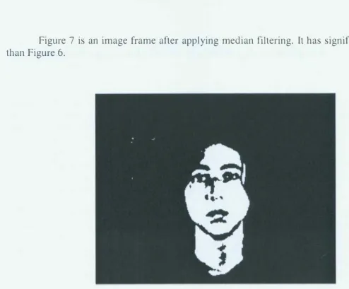
Figure 7 is an image frame after applying median filtering. It has significantly less noise than Figure 6 .

Figure 7. Filtered Image

•

•

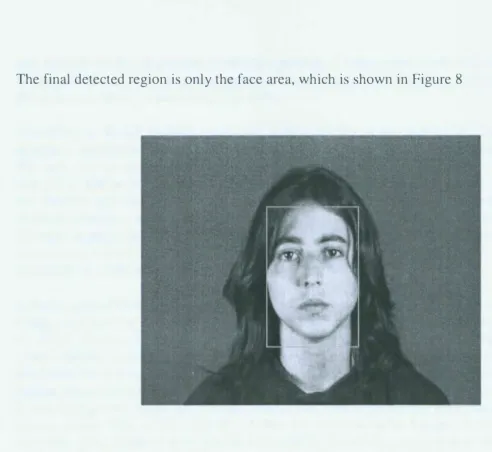
The final detected region is only the face area, which is shown in Figure 8

Figure 8. Final face detection

3.4 Facial expression segmentation:

There are 4 main features which are needed to be extracted from the face region.

1. Eye Brow contour 2 Cheek area

3. Nose area 4. Lip contour

These facial features have horizontal edges in the face. Kun Peng, et al. (2005) have used horizontal and vertical projections of the gradient image to determine the face width and the eye locations.

Eye locations, face size, and facial anatomy knowledge were combined to derive facial features such as lips, eyebrows, nose and cheek. Once facial feature areas are identified, tracking point positions on features are calculated.

•

•

•

•

row and the vertical projection detects the number of foreground pixels in each column. As seen in Figure 6, the horizontal projection would have a large count because the number of foreground pixels around the eye areas has a high value.

According to facial anatomy, eyes are located on the upper part of the face, and from face detection, the face height is known. By applying a horizontal projection on the gradient image of the face, the eye zone can be identified, because the pixels around the eye area will be more changeful. The peak of the horizontal projection is identified as the eye zone. Once we know the eye location and face width, we can determine the cheek zone, nose zone and lip zone based on the facial anatomy assumption and the vertical and horizontal projections. As seen in Figure 7, the vertical projection would have a large count because the number of foreground pixels around the nose and cheek area has a high value. Once the projections are found, the next step is to determine the motion in these zones .

•

Figure 9 shows the face image after the edge detection. The Sobel edge detection algorithm was used to detect edges. As seen in the Figure 9, edges are more prominent around the eye area and lip area. This face image is equally divided into upper half and lower half since we know the fact that eyes are on the upper part of the face and lips are on the lower part of the face. The upper portion of the face is further equally divided so that the left portion shows the left eye and the right portion shows the right part. The lower portion of the face shows the lips. This i shown in Figure 10.

t:agea image

Figure 9. Face after edge detection

up p e rleft Face upperRightF ace lowerHalfF ace

t

t

•

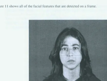
Figure 11 shows all of the facial features that are detected on a frame.

Figure 11. Facial features detection

The left eyebrow, right eyebrow and lips are detected using the horizontal and vertical projections on the binary edge images of the upper left, upper right and lower half section. Eyebrow detection is also based on the following three facts:

1) On the upper part of the face there are two main regions: 1) eyes, 2) eyebrow. The eyebrow region is the first region to have many edges

2) An eyebrow's length along the y dimension is a little less than the width of the upper left face or the width of the upper right face.

3) There is gap between the eyes and the eyebrows

•

t

There are five points on the lip as shown in Figure 12: 1) one on the outer left comer of the lip 2) one on the outer right comer of the lip 3) one on the middle part of the upper lip 4) two on the lower part of the lip.

There are total 3 points on each of the eyebrows as shown in Figure 13: 1) one on the outer left comer of the eyebrow 2) one on the outer right comer of the eyebrow 3) one in the middle of the eyebrow .

•·

Figure 12. Points on upper and lower lips

�:

•

t

Figure 14 shows a frame from the video with the tracking points superimposed. Figures 15 and 16 show the feature points that were found during tracking of an actual video sequence, and

Figure 14. Tracking points on face

.e

Figure 15. Points on upper and lower lips

�:

�1

Figure 17 shows the corresponding video frame from which the features were extracted and tracked.

Figure 17. Tracking points on face of a key frame

The nose and cheeks are detected based on the location of the eyebrows and lips. The nose region is detected by applying horizontal and vertical projections on the area above the lip region. The left cheek region is located below the left eye region and left side of the nose region. The right cheek region is located below the right eye region and right side of the nose region. Cheeks are always located below eyes and right and left side of a nose. The face width is also known, so based on face size, the nose location, and the eyebrow location, the cheek area is defined. The cheek area is a square area along with the nose in horizontal space, and below the eye area in vertical space.

Figure 18 shows the face edges before nose wrinkles are formed.

Figure 19 shows the frame where nose wrinkles are formed. Figure 20 shows the nose region .

•

Figure 19. Frame image where nose wrinkles are formed

Figure 21 shows the face edges after nose wrinkles are formed. It is obvious that there are more edges in the nose region of Figure 21 than of Figure 18. These frames show that the likelihood of nose wrinkles occurring during a facial expression is high.

Similarly, the cheek area should also have edges if the cheeks are raised. So instead of applying motion tracking, edge detection is again used to check for rai ed cheeks.

Figure 21. Edge detection after nose wrinkles are formed

3.5 Vocal feature segmentation

There are three key voice features that need to be identified from a shot: speech rate, pitch average, and pitch changes.

Pitch determination:

Pitch i an inherent part of the human voice. It is generally defined as the rate of vibration of the vocal chords. Pitch rises when vocal chords start to vibrate quickly. These vibrations and speed are dependent on the thickness and length of the vocal chords. Women tend to have higher pitches than men. Pitch is commonly referred to as sensations of frequencies; a high frequency

n

Xor P = log

L

(6) • Where x i+p = (i+p )1h _{signal in that frame}

n

=

Equation 6 is adopted from Zeng et al. (2004 ).

Pitch is detected from a window of the signal. This window is determined based on a frame rate and a sampling rate. The sampling rate is the number of signals of audio per second. For example, if a frame is captured every 0.04 seconds and the sampling rate is 22050 signals per second, then the window length is 0.04 * 22050 = 882.

From this window of signal values the autocorrelation value is calculated based on Equation 6. The pitch value is determined based on the highest value of XOR from this window. This method proved to be na·ive and did not work well. It will yield better results if the autocorrelation is applied on signals which the human auditory system perceives. To do this, Lyon's cochlear t model (available in the MATLAB Auditory Toolbox developed by Malcolm Slaney) was used (cobweb.ecn.purdue.edu/-malcolm/interval/1998-010/). The various parts of the human auditory system interact with each other and convert sound waves to neural firing (Lyon R. F., 1982). Lyon's auditory model describes the most important part of the human ear cochlea. The Auditory Toolbox contains LyonPassiveEar to implement this model. The output of this model is a vector proportional to the firing rate of neurons at each point in the cochlea. The output is stored as a two-dimensional array. The rows of this array represent one neuron's firing probability, and the • columns represent the firing probability on the auditory nerves at one time, as described in the

Auditory Toolbox guide. The cochlear output is a repetitive waveform, and we need to have a better representation of this waveform. A correlogram is an excellent way to summarize this periodicity. The Toolbox has a method called CorrelogramArray to compute the correlogram array. Pitch is computed from this correlogram array based on the autocorrelation method. This is also provided in the Auditory Toolbox as method CorrelogramPitch and is based on Equation 6.

t

Speech rate is calculated based upon the energy value of sound per each frame.

The logarithm of the energy is the value actually used and is computed by

Where N = number of frames

X

= i

n E = log

L

xf

i=l

•

Equation 7 is adopted from (Zeng, Z et al.,2004).

As discussed by Zeng et al. (2004) a frame is considered as speech if for any frame the log energy (E) is greater than the threshold value. This threshold value is derived based on training data .

3.6 Bayesian Network

A Bayesian network is a popular modeling tool to analyze complex problems. Understanding human emotion is a complex task which can help researchers in the area of human computer interaction. A Bayesian network is a valuable tool which involves probabilistic reasoning. Bayesian networks are very useful for predicting outcomes when a system has uncertain and/or incomplete information.

A Bayesian network is a probabilistic graphical model that represents a set of random variables and their conditional dependencies via a directed acyclic graph. A Bayesian network is useful when you have certain knowledge (prior probabilities) about your domain and you need to know uncertain values (posterior probabilities). It is based on Bayes' rule. Bayes' rule was named after Thomas Bayes who first provided the mathematical base for probability inference in "Essay • _{Towards Solving a Problem in the Doctrine of Chances" (1763).}

•

Bayes' rule is an expression of marginal probability and conditional probability, as shown in Equation 8. Conditional probability P(AIB) is the probability of some event A given the occurrences of some event B. Marginal probability is an unconditional probability P(A) of the event A regardless of whether event B occurred or not.

Where

P(AIB) =P(BIA)P(A) _P(B)

• P(A) = prior or marginal probability of A.

• P(AIB) = posterior or conditional probability of A, given B. • P(BIA) = posterior or conditional probability of B given A. • P(B) = prior or marginal probability of B.

(8)

•

•

based on his medical records. Based on this information, we can derive the probability of a person having an allergy given that he has a fever.

The posterior probability is

-Posterior probability= ( likelihood * prior )/ marginal likelihood

Definition: A Bayesian network consists of the following (Russel, R and Norvig, P., 1995): • A set of variables and a set of directed edges between variables

• Each variable has a set of mutually exclusive states

• The variables and the directed edges form a directed acyclic graph (DAG). (A directed graph is acyclic if there is no directed path Al ---+ ... ---+ An such that Al = An)

• To each variable A with parents Bl, ... ,Bn, there is attached conditional probability table P(AIB 1, ... ,Bn)

There are several advantages of using a Bayesian network for classification. The most important advantage of the Bayesian network is that it provides a probability framework, also, it is easy to interpret and unambiguous. A Bayesian network can also handle different data types like binary, discrete, and continuous. Another advantage is that it is easy to improve the Bayesian framework. One can always add more information in the network just by adding more nodes. The whole framework can be represented by a graph so that a human or a computer can easily understand the problem domain and dependencies. The disadvantage is that one needs to have perfect prior information of the problem domain. If the prior knowledge is wrong then it affects the whole network and the result becomes unreliable. It is also not sensible to build the Bayesian network for a very large application because as the number of nodes grows it becomes very expensive to calculate the posterior probability of the domain.

How to construct Bayesian network for emotional recognition:

Using Bayes' rule as show in Equation 8 we can calculate the posterior probability of specific facial expressions:

p (FE {i) I AU U)) = P( AU U) I FE U)). P( FE (i)) / p (AU U)) Where

P (FE Ci) I AU U>) = posterior probability of facial expression (FE) given an action unit (AU) P( AU U> I FE Ul) = likelihood of action unit given a facial expression

P( FE (il), P (AU (jJ) = prior probability of facial expression and action unit.

In case of visual features

AUu> = { inner eyebrow movement , outer eyebrow movement , upper lip movement , lower lip movement , lip corner , cheek , nose }

In case of vocal features

AU(i) = { Speech rate , Pitch average , Pitch changes }

• _{Given the prior and posterior probabilities, Bayesian analysis can be used to determine an}

•

•

•

emotional state; for example, the 'happy state'. Based on the facial action coding system (FACS), there are two features that can determine the happy state. 1) lip corners are pulled 2) cheek is raised.

The basic task here is to compute the posterior probability of the emotion given some observed events like lip corners are pulled and/or cheeks are raised. In this case, P(HappylJip_corner = true, cheek raised= true) needs to be calculated.

There are different algorithms to calculate the posterior probabilities. These algorithms are known as inference techniques.

Different inference techniques:

I) Inference by enumeration 2) Variable elimination algorithm

The following section discusses these inference techniques in more detail.

3.7 Bayesian Inference Techniques

•

According to Equation 9, a query P (Xie) to the network can be answered by,

where e = particular observed event y = nonevidence variable X = query variable

P(�)

L

a = normalization constant needed to make the entries in P(YIX) sum to I.

(9)

It is known that the full joint distribution represents the complete Bayesian network (Russell S. and Norvig P., 1995), as shown in Equation 10:

n

P(x1, ... . , Xn) =

n

( I 0) where P(x1 , .... ,x11) = P (X1 = X1 J\. .. J\. X11 = Xn)

parents(Xi) = specific values of the variables in Parents(Xi)

Equations 9 and 10 are adopted from (Russell, S and Norvig, P., 1995).

P(x,e,y) in the joint distribution can be written as products of conditional probabilities from the network. Therefore we can say that a query can be answered by computing sums of products of conditional probabilities from the network (Russell, S and Norvig, P:; 1995).

To calculate the joint probability, the nodes must be ordered in the expression in such a way that if node X2 is dependent on another node X 1, then X2 appears after XI in the joint. Ordering is important so that connections between nodes make logical sense. This requires starting with the causes and then adding the events they cause, and then treating those events as causes etc. This significantly reduces the complexity of computation.

Inference by enumeration is an exact method which requires summing over the joint distribution. This joint distribution size is exponential in the number of nodes. This is an expensive way to do inference.

•

•

•

all these variables before processing the query. Variable elimination can help avoid duplicate computation which makes it more efficient than inference by enumeration.

Below are the basic steps to construct a Bayesian network:

1) Random variables (graph nodes) are defined to represent domain. 2) Variable values are evaluated.

3) Using the basic knowledge about the domain define the dependency between the variables. (Draw arcs between nodes in the graph).

4) Define joint probability distribution if the network is really small. The joint probability distribution has all the information about the domain, but as the network grows, the joint probability distribution tends to become large and so avoid calculating needless dependency between nodes. Find out conditional independence between nodes.

•

•

•

•

•

•

Chapter 4: Approach

This thesis uses bimodal information (visual and vocal) to improve upon ex1stmg emotion recognition systems. The basic approach is to feed facial feature movements and audio feature information to their respective Bayesian networks. Output from both classifiers is used to make the final classification. The following sections provide more information on how facial features and audio features are measured and evaluated.

4.1 Facial Expression Classification Using A Bayesian Network

Below are the set of variables and their values for the facial expression classification Bayesian network. The variables represent the action units defined in Facial Action Coding System (FACS). FACS is a popular method for estimating and understanding facial behaviors. It was developed by Paul Ekman and W.V. Friesen in the 1970s. They examined and determined how the contraction of each muscle alone or in combination with other facial muscles changes the appearance of the face. Action units are the measurement units of FACS.

I. Inner Brow movement a. Brow raised

b. Brow lowered

C. Unaffected 2. Outer Brow movement

a. Brow raised b. Brow lowered C . Unaffected 3. Upper Lip movement

a. Upper lip raised b. Unaffected 4. Lower Lip movement

a. Lower lip lowered b. Unaffected

5 . Lip corner

a. Lip corner pulled b. Lip corner depressed C. Unaffected

6. Nose

a. Nose wrinkle b. Unaffected 7 . Cheek

a. Cheek raised b. Unaffected

guide, as shown in Table I below. For example, if the lip comers are pulled and the cheek is raised then the probability of the person laughing is high, therefore that person is happy.

Table I shows action units associated with emotions as per FACS guide

•

Inner eyebrow raised lowered raised unaffected unaffected

movement

Outer eyebrow raised lowered lowered unaffected unaffected

movement

Upper lip raised unaffected unaffected unaffected raised movement

Lower lip lowered unaffected unaffected unaffected lowered

movement

Lip corner unaffected depressed depressed pulled unaffected

Cheek unaffected unaffected unaffected raised unaffected

Nose unaffected unaffected unaffected unaffected wrinkled

Table I. Action Units associated with emotions as per FACS guide

These action units are measured by comparing key frame tracking points with the first frame • (neutral frame). The position of tracking points of both the neutral frame and the key frame is

stored in a structure. This structure has an x and a y position for each point from the left and right eyebrows and the upper and lower lips.

•

•

t

Facial Feature Tracked Point Threshold Result

lower lip y-position >2 lowered

lip corner x-position >4 pulled

lip corner x-position <2 depressed

upper Lip y-position <2 raised

inner Eyebrow y-position >2 lowered

inner Eyebrow y-position <2 raised

outer Eyebrow y-position >2 lowered

outer Eyebrow y-position <2 raised

nose Number of white >5 wrinkled

pixels

cheek Number of white >3 raised

pixels

Table 2. Facial feature action unit measurements

Threshold values are determined based on training data. A total 12 DaFEx emotional and 5 neutral videos were chosen. For each emotion video facial feature, movements were measured in pixels. 95% of total emotion videos showed that movements are within this threshold range. All neutral videos showed that movements do not meet threshold requirement. Count of white pixels from edge detected image area of nose is also stored and compared against neutral frame. Probability of wrinkle is high if count of white pixels in nose area is greater than then the count of white pixels from edge detected image area of nose of neutral frame. In order to consider nose wrinkle value true the count difference should be higher than 5. Similarly for cheek area the count of white pixels should be higher than 3.

Conditional probability values for each facial feature are described below. It uses the convention that false=l and true=2.

Table 3 shows conditional probability table (CPT) for lip comer (LC).

Emotion Probability Probability Probability of LC of LC being of LC being being unaffected pulled depressed

Angry=True 0.15 0.75 0.1

Angry=False 0.85 0.25 0.9

Sad=True 0 0.75 0.25

Sad=False 0 0.25 0.75

Happy=True 0.9 0.1 0

Happy=False 0.1 0.9 0

Table 3. CPT for lip comer

Table 4 shows conditional probability table for cheek.

Emotion Probability of Cheek Probability of Cheek being raised being unaffected

Happy=False 0.35 0.65

Happy=True 0.65 0.35

Table 4. CPT for cheek

Table 5 shows conditional probability table for nose.

Emotion Probability of nose Probability of nose having having wrinkled no wrinkles

Disgust=False 0.25

Disgust=True 0.75

Table 5. CPT for nose

Table 6 shows conditional probability table for lower lip.

Emotion Probability of Probability of lower lip lower lip lowered unaffected

Fear=False 0.15 0.85

Fear=True 0.85 0.15

Disgust=False 0.25 0.75

Disgust=True 0.75 0.25

•

•

•

•

•

•

Table 7 shows conditional probability table for upper lip.

Emotion Probability of Probability of upper upper lip raised lip unaffected

Fear=False _{0.15 0.85}

Fear=True 0.85 0.15

Disgust=False _{0.25 0.75}

Disgust=True _{0.75 0.25}

Table 7. CPT for upper lip

Table 8 shows conditional probability table for inner eyebrow (IE) .

Emotion Probability Probability Probability

of IE being of IE being of IE being

raised lowered unaffected

Angry=True _{0.2 0.7 0.1}

Angry=False _{0.8 0.3 0.9}

Fear=True _{0.8 0.1 0.1}

Fear=False _{0.2 0.9 0.9}

Sad=True _{0.7 0.2 0.1}

Sad=False _{0.3 0.8 0.9}

Table 8. CPT for inner eyebrow

Table 9 shows conditional probability table for outer eyebrow(OE).

Sad Probability Probability Probability

of OE of OE of OE

being being being

raised lowered unaffected

Angry=True _{0.3 0.7 0}

Angry=False _{0.7 0.3 0}

Fear=True _{0.7 0.3 0}

Fear=False _{0.3 0.7 0}

Sad=True _{0 0.6 0.4}

Sad=False _{0 0.4 0.6}

Figure 23 defines the Bayesian network for facial expression classification:

,,

"--~

movement

Inner eyebrow movement

•

~

.

..

Upper lip movement

Lower lip movement

~~

~

~

•

Lip corner

Figure 23. Bayesian network for facial expression classification

This thesis used the MATLAB Bayesian network toolbox which was written by Kevin Murphy (www.cs.ubc.ca/-murphyk/Software/BNT/bnt.html). This is an excellent tool to implement a probabilistic model. Also, it is very useful for research and rapid prototyping since the source code is very well documented.

4.2 Voice Classification Using A Bayesian Network

Below are the set of variables and their values for the speech emotion classification Bayesian network. Murray and Amott ( 1993) have described human vocal emotion effects. The random variables in the Bayesian network are chosen based on their classification and are relative to neutral speech.

1. Speech Rate

•

i

•

•

•

•

•

•

•

•

2. Pitch average a. High b. Low

3. Pitch changes a. Abrupt

b. Smooth upward inflections c. Downward inflections d. Normal

Table 10 shows the domain knowledge which is interpreted from the Murray and Amott (1993) summary of human vocal emotion effects. For example, faster speech rate and higher pitch average indicate a happy voice. Low pitch average and slower speech rate is an indication of a sad voice .

Fear Anger Sadness Happiness Disgust

Speech rate faster slightly slightly faster or very much

faster slower slower slower

Pitch high high low High low

average

Pitch normal abrupt low High low

changes

1

•

• The Bayesian network representation used for speech recognition is shown in Figure 24 .

•

•

•

•

•

•

•

Sad

Happy

Fear

/ '

Anger

�sgust

•

•

•

..

..

"'

"'

..

.,,..

Speech rate Pitch Average Pitch changes

Figure 24. Bayesian network for speech expression classification

Using this network we can compute the posterior probability of features nodes based on the vocal effects, and classify a sample facial expression according to which has the highest probability.

Conditional probability of each speech feature is calculated based on 15 training videos. Each speech feature value is calculated based upon the method described in above section. Probability is calculated based on each speech feature value and which emotion it belongs to. For example, if 4 out of 5 sad emotion video is having pitch average value as low then probability of pitch average feature for sad emotion is 0.8.

..

•

•

• Table 11 shows conditional probability table (CPT) for speech rate (SR) .

•

•

•

•

•

•

•

•

•

•

Emotion Probability Probability Probability Probability of faster of slower of slightly of slightly

SR SR faster SR slower SR

Angry=True _{0.1 0.1 0.7 0.1}

Angry=False _{0.9 0.9 0.3 0.9}

Happy=True _{0.5 0.5 0 0}

Happy=False _{0.5 0.5 0 0}

Sad=True _{0 0.2 0 0.8}

Sad=False _{0 0.8 0 0.2}

Fear=True _{0.8 0.1 0.1 0}

Fear=False _{0.2 0.9 0.9 0}

Disgust=True _{0 0.1 0 0.1}

Disgust=False _{0 0.9 0 0.9}

Table 11. CPT for speech rate

Table 12 shows conditional probability table for pitch average (PA) .

Emotion Probability Probability of PA of PA being high being low

Angry=True _{0.9 0.1}

Angry=False _{0.1 0.9}

Happy=True _{0.9 0.1}

Happy=False 0.1 0.9

Sad=True _{0.1 0.9}

Sad=False _{0.9 0.1}

Fear=True _{0.9 0.1}

Fear=False _{0.1 0.9}

Disgust=True _{0.1 0.9}

Disgust=False _{0.9 0.1}

Table 12. CPT for pitch average

-•

•

•

•

•

•

•

•

•

•

•

•

•

•

•

•

•

Table 13 shows conditional probability table for pitch changes (PC).

Emotion Probability Probability Probability

of PC of PC of PC

being high being low being abrupt

Angry=True 0 0 1

Angry=False 0.5 0.5 0

Happy=True 0.9 0.1 0

Happy=False 0.1 0.9 0

Sad=True 0.1 0.9 0

Sad=False 0.9 0.1 0

Disgust=True 0.1 0.9 0

Disgust=False 0.9 0.1 0

Table 13. CPT for pitch changes

The DaFEx database contains neutral (non-emotion) videos as well. Audio data of these neutral videos are used as a baseline to measure the sound feature values. Each person is different and can have different pitch and speech rate values even for a neutral emotion. These feature values are pre-calculated for each actor and supplied while measuring audio features of emotional videos. Pitch values are quantified using a statistical analysis. Statistical parameters such as mean, variance and standard deviation are calculated from the pitch vector. By comparing the standard deviation and variance of pitch values of emotional audio to the neutral base line value we can determine whether a person's pitch changes are high or low. The mean value of an emotional pitch is compared to the mean value of a neutral audio. Similarly, the speech rate values are also compared to neutral.

The pitch average can be high or low. If the mean value of an emotional pitch is higher than the mean value of a neutral pitch of the same actor, then the pitch average feature is marked as high. If the mean value of an emotional pitch is lower than the mean value of a neutral pitch of the same actor, then the pitch average feature is marked as low. The pitch value is computed based on the method described in section 3.5 .

•

•

speech rate of a neutral video but less than 20% of the speech rate of a neutral video, then speech rate is marked as slightly fast. If the difference between the speech rate of an emotional video and a neutral video is greater than 20% of the speech rate of a neutral video, then speech rate is marked as faster.

If the difference between speech rate of neutral video and emotional video is less than 20% of speech rate value of neutral video then speech rate is marked as slower. If the difference between speech rate of neutral video and emotional video is less than 30% speech rate value of neutral video then speech rate is marked as very much slower. These threshold values are determined based on doing analysis on training videos where speech rate values were derived and compared to determine the threshold value.

Table 14 shows how vocal feature action units were measured.

Vocal Feature Threshold Criteria Result

Speech Rate >20% Fast

Speech Rate Between 5% to 20% Slightly fast

Speech Rate < neutral video value Slow

Speech Rate Between 20% to 30% Slightly slow

Speech Rate <30% Very slow

Pitch Average Higher than neutral Hjgh

video value

Pitch Average Lower than neutral Low

video value

Pitch Changes Higher than neutral High

video value

Pitch Changes Lower than neutral Low video value

Table 14. Vocal feature action unit measurement

4.3 Evaluation

This thesis has used the DaFEx (Database of Human Facial Expressions) database (http://i3.fbk.eu/en/dafex). DaFEx is composed of 10

and in utterance and non utterance condition. This thesis does not use the non-utterance videos, the low and medium intensity videos, or the surprise videos.

Below are the main characteristics of DaFEx videos:

1) Videos have all frontal views and only frontal view faces are analyzed. 2) Videos have one person at a time showing emotion in the video. 3) Videos are taken under normal lighting condition.

4) All are indoor shots.

5) While taking video, position the subject so that only face and neck is seen. 6) Video format is .avi.

7) Videos are already labeled by having 80 subjects classify the emotion expressed in the videos

8) There are 25 frames per second captured in the videos.

9) Image resolution is 360 x 288.

Probability values from both classifications (facial and vocal) were derived as shown above. The DaFEx video database ranged in gender and age are tested. Results are assessed by counting the true positive, false positive and false negative classification. Ground truth is provided by the author of the DAFEX database. Ground truth data is stored for the verification purposes. Actual results are compared to the ground truth already labeled in the database.

A confusion matrix is a helpful visualization tool which can show the true performance of the classifier. The confusion matrices will have results from the 1) facial feature classifier, 2) vocal classifier and 3) combined visual and vocal classifier.

•

•

•

Chapter 5: Results and Discussion

5.1 Overall Results of the Three Types of Classifiers

This thesis found that emotion recognition through the use of vocal and facial features depends upon the type of classifier used (facial, vocal, or both). From Table 15 we can see that happy and disgust emotions are classified better with just facial features, while sad, angry and fear emotions are classified better with vocal features.

.... Q.)

r./'J r./'J C's)

u

Percent Correct Classification of Emotions by Classifier Type

---

Facial 80% 60% 70% 50% 60%

Feature

Vocal 70% 85% 40% 70% 70%

Feature

Table 15. Summary of classification results

Table 15 shows summary of classification results by each classifier. Happy and disgust emotion was detected at least 10% better by facial classifier while sad, fear and angry

• emotion was detected at least 10% better by vocal classifier. This shows it is not possible to detect all the emotions using just one modality and additional semantic information can help improve classification of certain emotions.

•

•

•

•

•

•

•

Table 16 shows classification results by facial feature classifier.

VJ "O (1) i.C ·;;;_VJ �

u

---

Actual expression (Ground truth)

Happy Sad Disgust

80%

-

-

5% 5% 70%

10% 30% 10%

5% 5% 10%

Angry Fear

20% 14%

25% 17%

-

-50% 28%

5% 60%

Table 16. Confusion matrix of facial feature classification results

A Bayesian network is an optimal classifier provided it is properly trained and modeled. The

happy emotion is detected when the lip comer is pulled and the cheek is raised. Lip comer movement detection and cheek detection rate is 80% and for all these cases, the happy emotion was detected. It did not work when the nose region overlapped with the cheek region, and so the action unit was classified as nose wrinkle. Hence, the emotion was misclassified as disgust instead of happy. Angry was also misclassified due to subtle cheek movements and the fact that lip comers were not identified correctly on the key frame.

The sad emotion is based on eyebrow movements and lip comer depressed action units. The sad and anger emotions have very similar visual features, where the only difference is with the inner eyebrow movement. In the case of sadness, the inner eyebrow is raised sometimes while in the case of anger, the inner eyebrow is lowered. So if inner eyebrow movements are not accurately identified, then the classifier can get confused between these two emotions.

Disgust emotion has very unique facial feature - nose wrinkles. No other emotion is supposed to exhibit this action unit. Nose wrinkle detection rate is 80% but in some cases this expression lasted briefly, only for 2-3 frames. It can go undetected if the key frame is not captured during this brief expression.

The facial feature classifier has an average performance of 50% and 60% for the angry and fear emotions respectively. Their detection is based mostly on eyebrow movements. In some cases actors did not display any eyebrow movements at all and some cases movements were pretty subtle to track. Also threshold values are determined based on the assumption that there should not be any head movement. In some cases heads were tilted and it can interrupt with tracking

•

•

•

•

•

•

•

•

movements. One way to improve the model would be to create a 3D wire frame model that captures the possible motions of facial muscles (Dornaika F. and Davoine F., 2008).

VJ <!'. "O <l) VJ VJ ell

Actual expression (Ground truth)

---

Happy 70%

-

Sad

-

-

Disgust 10% 5% 40% 10% 15%

Angry 10% 5% 10% 70% 5%

Fear 10% 5% 12% 5% 70%

Table 17. Confusion matrix of vocal features classification results

The vocal classifier detection rate for the sad emotion is 85%. This emotion has low energy and slower speech rate. Both features were detected 90% of the time successfully for this emotion . Sad and disgust both has similar pitch features which is why the classifier confused these emotions with each other.

The vocal classifier detection rate for the happy, angry and fear �motion is 70%. The happy emotion was confused with angry because both have similar speech rate and pitch average .

The detection rate for the disgust emotion by the vocal classifier is just 40%. Disgust is a complex emotion and its vocal feature measurements are similar to the sad emotion. The only difference is that disgust has speech rate lower than sad. Even just by hearing disgust speech without knowing the language it was hard to conclude this emotion. This suggests the need to derive linguist information as well from the speech. It may be desirable to tag certain words with certain emotions; for example, 'sorry' with sad or 'wow' with happy. This is another research area where future work may enhance the performance of the classifiers. The more features computers can extract, the better the emotion recognition would likely be. In the current scope of this research we can conclude that key features like speech rate and pitch values can derive emotions like sad. Adding more features may help recognize certain complex emotions such as disgust.

•

•

•

•

•

•

•

•

•

u

Actual expression (Ground truth)

---

Happy 75%

-

Sad

-

Disgust 7.5% 5% 55% 10% 15%

Angry 10% 17.5% 10% 60% 16.5%

Fear 7.5% 5% 11% 5% 65%

Table 18. Confusion matrix of facial feature and vocal features combined

ROC curves below illustrate the results obtained for the classifiers used separately, and then combined. The ROC curve shows the false positive rate (FPR) on X axis and true positive rate (TPR) on Y axis. The closer the curve follows the Y axis the more accurate the test since it means we have more true positive tests than false positives. The area under the curve also provides val