Modelling a Borehole Subjected to Fluid Pressure
A.GOLSHANIa,T.TRAN-CONGb
aComputational Engineering and Science Research Centre (CESRC), University of
Southern Queensland, Toowoomba 4350, Australia
golshani@usq.edu.au
bComputational Engineering and Science Research Centre (CESRC), University of
Southern Queensland, Toowoomba 4350, Australia
trancong@usq.edu.au
Abstract
Fluid pressure inside a borehole produces hydraulic fracture and damage zones in the vicinity of the borehole. These fractures result from stress concentrations around the borehole. The results of numerical simulation of a borehole subjected to fluid pressure using a micromechanical damage model [2] are presented in this paper. It is observed that tensional concentrated stresses are generated around the bottom of the borehole by the applied fluid pressure. Furthermore, fractures develop from the corners of the bottom of the borehole.
Introduction
In oil and gas production, a process known as hydraulic fracturing is often used. Hydraulic fracturing involves pumping a fluid under pressure into a reservoir. When the pressurized fluid enters the reservoir it produces stress concentration in the surrounding rock which may lead to rock fracture. The fracture creates a conductive path for the production to flow towards the reservoir.
The fracture growth in the vicinity of a borehole is largely controlled by rock failure. In order to maximize the efficiency of hydraulic fracturing method, it is of great importance to investigate the fracturing process in rock under fluid pressure and to predict the pressure needed to cause the desired fracture.
In this paper, we study mechanical response of rock around a vertical borehole drilled in rock under fluid pressure by using the micromechanical damage model proposed by Golshani et al. (2006). Special attention will be paid to the fracture process under compression in the surrounding rock in terms of microcracking which takes place in association with inelastic deformation.
Overview of micromechanical damage model
In this model, the rock matrix is regarded as an elastic solid with N groups of microcracks
orientationθ(i), the number density of the microcracks ρ(i), and the average microcracks
length 2c(i). θ(i) is the inclination angle of the unit vector n(i), normal to a microcrack, to
the global axis x1 (see figure 1). In the following discussion, “´” indicates quantities in the
local coordinate xi′−axes.
Figure 1: A single microcrack
By assuming that microcrack growth occurs in tensile mode I [1, 2], the stress intensity
factor KI for a single microcrack with respect to local axes x′i(i=1,2)is approximated by:
t
I c
K =− π σ′ (1)
where σ ′t is the tensile stress acting normal to the microcrack surface, and is expressed as:
22 22 f(c)S
t′ σ= ′ + ′
σ (2)
It should be noted that the compressive stress is taken to be positive. The first term on the right hand side of Eq. (2) stems from the far field compression, hence it takes a positive (compression) in a common case. This means that the first term acts as an inhibiting factor for microcracking. The second term is the tensile stress, which is locally generated as a result of the inhomogeneity of rock and sliding movement on asperities. Following the suggestion by Costin [1], we assume that the local tensile stress increases proportionally to
the deviatoric stress S22′ , and that f(c) is a proportionality coefficient depending only on
half the microcrack length c. It is of particular importance to point out that the local tensile
stress must decrease as the microcrack grows. Otherwise, the microcrack would propagate
without any limit as soon as the stress intensity factor KI reaches the fracture
toughnessKIC. This unsatisfactory situation is easily avoided if the proportional coefficient
) (c
f is inversely proportional to half the microcrack length:
c d c
f( )= / (3)
where d is a typical length scale of material such as grain size, and is experimentally
determined (see Golshani et al., 2006).
2c
θ
n
1
x′
2
The stress-induced microcrack growth takes place in tensile mode I when the following relation is satisfied:
0
= − ′ − =
− IC t IC
I K c K
K π σ (4)
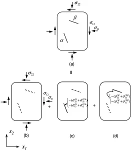
Equations (4) was formulated for a single microcrack and the effect of neighboring microcracks was not considered. In order to evaluate the elastic interaction among neighboring microcracks, we use the so-called pseudo-traction method developed by Horii and Nemat-Nasser [3, 4]. For simplicity, we first consider an infinite plate with two
microcracks αand β with lengths 2 andcα 2 , both of which are subjected to far field cβ
stresses (see figure 2). This problem is elastically analyzed by decomposing it into three
sub-problems; i.e. a homogeneous sub-problem and two sub-problems α andβ, as shown
in Figure 2. There is no microcrack in the homogenous sub-problem, which is subjected to
the same far field stresses as the original problem (i.e. σ11, σ22 and σ12). In the
sub-problemα andβ, we deal with a single microcrack under zero stresses, individually. The
traction-free condition must be satisfied on the surface of the microcracks in the original
problem since the microcracks αand βare assumed to be open. To do this,
)
( 22 22
α
α σ
σ′ + ′P
− and ( 12 12 )
α
α σ
σ′ + ′P
− must be applied to the surface of the microcrackα in
the sub-problemα . Here, σ α
22
′ and σ α
12′ are the stresses at the position of microcrack α
arising from the far field stresses in the homogenous problem, and σ Pα
22′ and
α
σ P
12′ , called
pseudo-tractions, stand for the stresses at the position of microcrack α in sub-problemβ.
That is, the pseudo-tractions are generated by microcrack β through elastic interactions
between the microcracks αand β.
The pseudo-tractions are calculated such that all the boundary conditions for the original problem are satisfied:
{ }
σ′Pα =[ ]{ } { }
γ′αβ(
σ′β +σ′Pβ)
(5)where
{ } {
Pα Pα Pα Pα}
Tσ σ σ
σ′ = 11′ , 22′ , 12′ ,
{ } {
}
T β β β
β σ σ σ
σ′ = 11′ , 22′ , 12′ , and
[ ]
αβ
γ ′ is a 3×3 matrix
and each element of which is a function of the position vectors
x
α andx
β of the centersof microcracks αand β, their half lengths (cαand cβ), and the inclination angle θαβ
between β
1
x′ and α
1
x′ . Eq. (5) is tentatively called the consistency equation in the sense that
stress boundary conditions are taken into account. If more details are necessary, readers should refer to the papers by Horii and Nemat-Nasser [3, 4], Okui et al. [6], and Golshani et al. [2].
Figure 2: Decomposition of (a) the original problem into (b) the homogeneous problem and (c) and (d) two sub-problems
equation [6]: Consider N groups of microcracks, we can rewrite Eq. (5) with respect to the
global axesxi(i=1, 2), as follows:
{
}
[
]
(
{
} {
}
)
() 1 ) ( ) ( ) ( ) ( ) ( ) ( ( , , , ) ( ) ( ) )( N i
i V i P i i i i i
P xα ρ γ c θ xα xβ σ xβ σ xβ dxβ
σ β αβ
=
+
= (6)
Considering the effect of the interaction among microcracks, the stress intensity factor equation (Eq. (1)) can be rewritten as follows:
+ + 22 σ 11 σ
=
α βx
2x
1 22 σ 11 σ 12 σ 12 σ ′ + ′ − ′ + ′ − ) ( ) ( 12 12 22 22 α α α α σ σ σ σ P P ′ + ′ − ′ + ′ − ) ( ) ( 12 12 22 22 β β β β σ σ σ σ P P (a)(b) (c) (d)
+ + 22 σ 11 σ
=
α βx
2x
1 22 σ 11 σ 12 σ 12 σ ′ + ′ − ′ + ′ − ) ( ) ( 12 12 22 22 α α α α σ σ σ σ P P ′ + ′ − ′ + ′ − ) ( ) ( 12 12 22 22 β β β β σ σ σ σ P P (a)′ + ′ − ′ + ′ + ′ + ′ − = ′ ′ 2 ) ( ) ( ) ( ) ( ) , ,
( 22 22 11 11
22 22 P P P P
I c c f c
K σ σ π σ σ σ σ σ σ (7)
It is assumed that the rock matrix remains elastic in the entire process so that the inelastic deformation arises from opening of microcracks. Since the matrix is elastic, the stress-strain relationship is given by:
) (
: ε ε
σ =De t− (8)
where De is the elastic modulus tensor, εtis the total strain tensor and ε is the inelastic
strain tensor arising from the opening of microcracks. The symbol
()
: stands for the innerproduct. The inelastic strain caused by the microcracks belonging to the i-th group is
obtained in the local axesx′i(i=1, 2) as:
[ ] [ ]
u u n dxn i i i
c
c i
i ′ ⊗ ′ + ′ ⊗ ′ ′
= ′ −( ) ) ( ) ( ) ( ) ( ) ( ρ
ε (9)
where n′(i)is the unit vector normal to the microcrack, and
[ ]
(
())
2 2 ) (
2 ( )
i i
u u
u′ = ′+ − ′− is the
opening displacement where ′+
2
u and ′−
2
u are the displacements on the positive and negative
sides of the microcrack given as:
[ ]
( ) ( ) ( )2
1 ()
1 2 1 2 ) ( ) ( 2 i t i i c x x c G
u′ =−κ+ − ′ σ′ ′ ≤ (10)
where G is the shear modulus, and
κ
is the Lame constant [5].The inelastic strain arising from opening the i-th group microcracks is formulated in terms
of the average length of microcracks 2c(i), microcracks orientation θ(i), number density of
microcracks ρ(i), and the applied stresses σ [2]. The inelastic strain arising from all
microcracks is calculated by summing Eq. (10) with respect to the global coordinate axesxi(i=1, 2):
{ }
{
}
= = N i i i i c 1 ) ( ) ( ) ( , , , )( θ ρ σ
ε
ε (11)
We now have governing equations for analyzing stress-induced behaviour of brittle rock; i.e., microcrack growth law (4), consistency equations (6) and constitutive equations (8).
Unknowns are σ, c and σP. The initial values of the unknowns are given by solving
solved the governing equations on a numerical basis. Three-node triangular elements were used, in each of which the displacement, the interaction stresses and the length of the
microcracks belonging to the i-th group are constant.
Simulation of a borehole subjected to fluid pressure
In this study, a single borehole in Inada granite was considered. A rectangular region (1000
mm
×
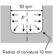
1000 mm) with a vertical borehole of 50 mm diameter and 500 mm depth was [image:6.612.252.359.284.395.2]analysed. The dimensions of the bottom of borehole are shown in figure 3.
Figure 3: Dimensions of the bottom part of the borehole
The region was meshed using triangular elements. The mesh consisted of 297 nodes and 496 elements as shown in figure 4. All parameters in the governing equations were selected as those for Inada granite (see Golshani et al., 2006). Inada granite elastic properties are:
Young’s modulus E=73GPa and Poisson’s ratio ν =0.23. Fracture toughness and length
parameter for Inada granite were chosen as 2.5MPam1/2 and 0.34 mm, respectively and in
the simulation we only considered vertical microcracks with initial length of 0.56 mm and number density of 0.0525. To model the effect of fluid pressure on stress concentration and
fracture around the borehole, uniform pressure p was applied inside the borehole.
Figure 5 shows the distribution of the normalized tensile stress around the borehole at
failure (p=55MPa). It was found that the applied pressure (p) results in large tensile
stress in rock mass especially at the bottom of the borehole, which is a stress raiser.
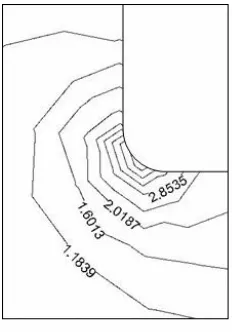
The contours of the maximum tensile stress around the bottom of the borehole at failure are
shown in figure 6. It is observed that tensile stress with a magnitude 400% of p appeares
near the corner of the borehole. Consequently, microcracks develop at the bottom of the borehole starting from the corners (see figure 7).
Figure 4: Finite element mesh
Figure 5: Distribution of normalized maximum stress at failure
[image:7.612.195.415.429.617.2]Figure 6: Contours of normalized maximum stress for borehole stub
Figure 7: Distribution of normalized microcrack length at failure (cris half length of the
[image:8.612.191.416.412.601.2]Conclusions
Concentration of stresses at the bottom of the borehole under fluid pressure is crucial to understanding the propagation of fractures around the borehole. Numerical simulation of a borehole subjected to fluid pressure using a micromechanical damage model [2] indicates that the applied fluid pressure results in large tensile stresses at the bottom of the borehole which is a stress raiser. Under such large tensile stresses microcracks develop at the bottom of the borehole starting from the corners.
Acknowledgement
This work is partially supported by the Australian Research Council. This support is gratefully acknowledged.
References
[1] Costin, L.S., A microcrack model for the deformation and failure of brittle rock. J.
Geophys. Res., 88, B11, 9485-9492 (1983).
[2] Golshani, A., Okui, Y., Oda, M. and Takemura, T., A micromechanical model for brittle failure of rock and its relation to crack growth observed in triaxial compression tests
of granite. Mechanics of Materials, 38, 287-303 (2006).
[3] Horii, H. and Nemat-Nasser S., Compression-induced microcrack growth in brittle
solids: axial splitting and shear failure. J. Geophys. Res., 90, 3105-3125 (1985a).
[4] Horii, H. and Nemat-Nasser S., Elastic fields of interacting inhomogeneities. Int. J.
Solids Struct., 21, 731-745 (1985b).
[5] Nemat-Nasser, S. and Hori, M., Micromechanics: overall properties of heterogeneous materials. North-Holland, Netherlands, 687 (1993).
[6] Okui, Y., Horii, H. and Akiyama, N., A continuum theory for solids containing