B.I. Henry∗ and T.A.M. Langlands†
Department of Applied Mathematics, School of Mathematics, University of New South Wales, Sydney NSW 2052, Australia.
S.L. Wearne‡
Laboratory of Biomathematics, Department of Neuroscience, Mount Sinai School of Medicine, New York, New York. 10029-6574.
(Dated: February 25, 2008)
Cable equations with fractional order temporal operators are introduced to model electrotonic properties of spiny neuronal dendrites. These equations are derived from Nernst-Planck equations with fractional order operators to model the anomalous subdiffusion that arises from trapping prop-erties of dendritic spines. The fractional cable models predict that postsynaptic potentials propa-gating along dendrites with larger spine densities can arrive at the soma faster and be sustained at higher levels over longer times. Calibration and validation of the models should provide new insight into the functional implications of altered neuronal spine densities, a hallmark of normal ageing and many neurodegenerative disorders.
PACS numbers: 87.19.ll,05.40.-a,87.15.Vv,87.16.dp
Most of the brains grey matter is composed of spiny dendrites – the substrate for the interconnected neuronal networks that underlie cognitive function. Dendritic pro-cesses respond to synaptic inputs by relaying postsynap-tic potentials to the cell body or soma. The potentials are summed at the soma and the cell fires an action po-tential or spike if a threshold popo-tential is exceeded. The interspike interval determines the firing rate of nerve cells which is critical for normal cognitive functioning. An ongoing dialogue between theory and experiments over many decades has revealed the detailed electrotonic prop-erties of neuronal dendrites and dendritic trees [1]. The centrepiece of this is the cable equation [2, 3]
rmcm ∂V
∂t =
drm
4rL ∂2V
∂x2 −V +rmie, (1)
which models the spatio-temporal evolution of the mem-brane potentialVm, relative to the resting membrane
po-tential Vrest, along the axialxdirection of a cylindrical
nerve cell segment. The other parameters in the model represent; specific membrane resistancerm, longitudinal
resistivity rL, membrane capacitance per unit area cm,
diameter d, and an external injected current per unit areaie. In an infinite length cable described by Eq.(1)
the steady state voltage attenuates in space by a factor 1/eover a distance ofλ =qdrm
4rL and the spatially ho-mogeneous voltage for a membrane patch attenuates in time by a factor 1/e over a time τ = rmcm, so that λ
andτ are referred to as the space constant and the time constant for the dendrite. In Eq.(1) rm, rL and cm are
model parameters to be fit to experimental data butcm
is often taken to have a fixed value. The cable equation can be obtained phenomenologically by associating elec-trical properties with the cell membrane [3] or derived physically from the Nernst-Planck equation for
electro-diffusive motion of ions [4].
Over the past few decades research on neuronal drites has intensified [5] due to the discovery that den-drites are highly active, with complex electrical and bio-chemical signaling depending on both local spine struc-ture and density [6, 7], and on voltage-gated ion channels [8]. These processes present challenges to the cable model [9]. In this letter we consider refinements of the passive cable model (voltage gated ion channels are ignored) to incorporate dendritic spines (small protrusions extending 2µmor less out from dendritic branches, typically a few
µmin diameter). Spines are particularly prevalent along inhibitory Purkinje cells in the cerebellum (≈105spines per cell) and most excitary cells in the neocortex (≈104 spines per cell) [9]. The standard way to model the ef-fects of spines in the passive cable model is to reduce the membrane resistance and to increase the membrane capacitance, for an equivalent but smooth dendrite, by a factor proportional to the increased membrane surface area due to spines [9]. In this modification the time con-stant for the dendrite is unaffected by spines but the space constant is reduced, thus the steady state voltage should attenuate more strongly in space along spiny, rel-ative to smooth, dendrites [9, 10].
A recent study [11] on spiny Purkinje cell dendrites showed that spines trap and release diffusing molecules resulting in anomalously slow molecular diffusion, along the axial direction (through the cytoplasm). The diffu-sive spatial variancehr2(t)iof an inert tracer was found to evolve as a sub-linear power law in time, i.e.,hr2(t)i ∼tα
spiny dendrites, and we investigate the solutions of the fractional cable equations to provide new insights into the electrotonic effects of the trapping properties of spines. The scaling parameters that quantify the anomalous dif-fusion appear as parameters in the fractional cable equa-tions and significantly impact both spatial and temporal electrotonic properties in unanticipated ways.
The simplest model for anomalous diffusion replaces the diffusion constant D with a time-dependent diffu-sion coefficient Dαtα−1 in the standard diffusion equa-tion. This models fractional Brownian motion (fBm) that can be derived from a Langevin equation with a friction memory kernel and power law correlated noise [12]. A different model for anomalous diffusion at the macroscopic level includes a temporal derivative with fractional order 1−α operating on the spatial Lapla-cian in the diffusion equation [13]. This fractional equa-tion has been derived from mesoscopic continuous time random walks (CTRWs) with a power law waiting-time distributionψ(t)∼t−(1+α)[13]. The power law waiting-time is generic for random walks amid traps with an ex-ponential distribution of trap binding energies and ther-mally activated trapping times [14]. In the absence of experimental evidence to the contrary, it is prudent to consider both fBm and CTRW based anomalous diffu-sion models in fitting experiments [15, 16].
The Nernst-Planck equation is the fundamental macro-scopic model for the micromacro-scopic motions of ions in nerve cells. This model takes into account random motions of the ions as well as the drift of ions due to the electric field of the membrane potential (due to different ionic con-centrations inside and outside the cell membrane). As a starting point, to model anomalous electro-diffusion, we consider the following variant of the Nernst-Planck equation:
∂Ck
∂t =Dk(γk, t)∇
2C
k+∇.
z
kF
RT Dk(γk, t)Ck∇Vm
.
(2) In this equation,Ck is the concentration of thekth ionic
species,F is the Faraday constant,Ris the universal gas constant, andT is the temperature. The difference be-tween this model and the standard Nernst-Planck equa-tion is thatDk(γk, t) is not a constant for a given species k but is a parameterized time-dependent operator with scaling parameter 0 < γk ≤ 1. As discussed above we
consider the two possibilities related to fBm and CTRWs respectively: i)
Dk(γk, t) =Dk(γk)γktγk−1 (3)
whereDk(γk) has units ofm2s−γk and ii)
Dk(γk, t) =Dk(γk) ∂1−γk
∂t1−γk, (4)
where ∂1−γ
∂t1−γ is the Riemann-Liouville fractional
deriva-tive operator defined by
∂1−γ
∂t1−γY(t) =
1 Γ (γ)
∂ ∂t
t
Z
0
Y(t′) (t−t′
)1−γ dt
′
. (5)
In the following it is also useful to define the ‘normalized’ operatorsD∗(γ
k, t) =Dk(γk, t)/Dk(γk). Importantly, in
both the standard Nernst-Planck equation (γ = 1) and the fractional Nernst-Planck equations (0< γ <1) the effects of ionic diffusion are not isolated to the Laplacian term but they are also manifest in the drift term, through the dependence on the diffusion ‘constant’. It follows that even if concentration gradients are sufficiently small for the Laplacian term to be neglected, alterations in the environment that affect ionic diffusion would also affect the drift term. A second point to note is that in the fractional Nernst-Planck models the electric field force is a function of the ionic concentrations. As a result these models cannot be derived from CTRWs via frac-tional Fokker-Planck equations with external time inde-pendent forces [17, 18]. The fractional Nernst-Planck models do, however, capture this effect; variations in the time-dependent force field are driven by the same tempo-ral operator that affects variations in the time-dependent ionic concentrations. This contrasts with the fractional Fokker-Planck equations with external time-dependent force fields where an effective temporal subordination of the external force to the random walks is not appropriate [19].
The standard passive cable equation for a cylindrical nerve cell segment, with diameter d much smaller than the length ℓ, has been derived by Qian and Sejnowski [4] from the standard Nernst-Planck equation. We fol-low this approach in deriving the fractional cable models for spiny dendrites. First we integrate Eq.(2) in axially symmetric cylindrical coordinates over the circular cross-section of the neuron, with zero flux of ions at the centre. This results in
∂Ck
∂t =D
∗(γ
k, t)
Dk(γk) ∂2C
k ∂x2
+ zkF
RT ∂ ∂x
Dk(γk)Ck ∂Vm
∂x
−4dJk
r=d2 (6)
where x is the longitudinal coordinate, r is the radial coordinate andJk denotes the radial flux of ionic species kacross the membrane. As in the standard cable theory we model the membrane potential as [20]
Vm(x, t) =Vrest+ F d
4cm
X
k
zk(Ck(x, t)−Ck,rest) (7)
whereCk,restis the resting concentration of thekthionic
species. We also follow the standard assumption that the axial ionic concentration gradients are small (∂Ck/∂x≈
0), but the prefactor F d
addition we assume that the trapping effects due to the geometry of spines are similar for different species of mo-bile ions (γk ≈γ). Using these results in Eq.(6) we obtain
cm ∂Vm
∂t =D
∗(γ, t)
d
4rL ∂2V
m ∂x2
−im+ie (8)
where
1
rL(γ)
= F 2
RT
X
k
z2kDk(γ)Ck, (9)
defines a modified longitudinal resistivity rL(γ) with
units of Ωmsγ−1,i
m=P k
zkF Jk is the total ionic
trans-membrane current per unit area, andiehas been included
as an injected current per unit area.
As an alternative to the physical derivation above, the fractional cable equation, Eq.(8), can be obtained phe-nomenologically by combining the standard current con-tinuity equation
cm ∂Vm
∂t =
d
4
∂IL
∂x −im+ie (10)
with the longitudinal current, IL, described by a
frac-tional variant of Ohm’s Law,
IL=−D∗(γ, t)
1
rL(γ) ∂Vm
∂x . (11)
Allowing for a similar fractional flux for the ionic trans-membrane current we write
im=α(κ)D∗(κ, t)
Vm−Vrest rm
(12)
where κ is the exponent characterizing the anomalous flux across the membrane and α(κ) is an additional pa-rameter with units ofs1−κ. It is possible to absorbα(κ)
into a modified specific membrane resistance rm(κ) = rm/α(κ), identifyingα(κ) as the effect of anomalous flux
across the channels on the specific membrane resistance, and α(1) = 1. The fractional order operator D∗(κ, t) would also apply to any external current ie carried by
ions traversing the membrane. Equations (11) and (12) can be interpreted as either an aged linear response [21] or a retarded linear response [22], ifD∗(κ, t) has the form of Eq.(3) or Eq.(4) respectively.
Equations (8) and (12) can be combined to arrive at the linear fractional cable equation
rmcm ∂V
∂t =
drm
4rL(γ)D
∗(γ, t)
∂2V ∂x2
−α(κ)D∗(κ, t)(V −r
mie), (13)
where V =Vm−Vrest. The above model yields a
non-trivial steady state solution if the exponentsγ andκare equal. In the following we consider that a homeostatic
control mechanism could operate to achieve this balance, resulting in a spatially varying steady state membrane potential that only differs from that for the standard ca-ble equation through the parametersrL(γ) andα(γ). To
investigate further solutions of Eq.(13) it is useful to con-sider the explicit dimensionless forms, related to Eqs.(3) and (4) respectively:
∂VI
∂T =γT
γ−1∂2VI
∂X2 −µ
2κTκ−1(V
I−ierm) (14)
and
∂VII
∂T =
∂1−γ ∂T1−γ
∂2V
II
∂X2 −µ
2 ∂1−κ
∂T1−κ(VII−ierm) (15)
where T = t
τm is the dimensionless time variable,X =
xτ1−
γ 2
m /
q
drm
4rL is the dimensionless space variable, µ 2 =
α(κ)τκ−1
m is a dimensionless function ofκ, and the
sub-scriptsIandII are used to differentiate the two anoma-lous diffusion models. Equation (14) can also be derived from a fractional Nernst-Planck equation with a frac-tional order temporal derivative operating on the con-centration field but not the time varying electric field [23].
The fundamental solutions of Eq. (14) and Eq. (15) in the case of infinite cables with no external current are as follows:
GI(X, T) =
1 √
4πTγexp
−X
2
4Tγ −µ
2Tκ
(16)
and [24]
GII(X, T) =
1 √
4πTγ
∞ X
j=0
−µ2Tκj
j!
×H12,,20
X2 4Tγ
1−γ2+κj, γ
(0,1), 12+j,1
, (17)
whereH is a Fox function [25]. Both of these solutions reduce to the standard fundamental solution for an infi-nite cable in the case γ =κ = 1. In the remainder of this letter we consider solutions for γ = κ 6= 1. Solu-tions withγ6=κare described elsewhere [23]. GI(X, T)
withγ=κis identical to the fundamental solution of the standard cable equation, but at a later time. By contrast
GII(X, T) with γ=κ(see Fig. 1., left) is characterized
by a sharp peak and a heavy tail and is subordinated to the fundamental solution of the standard cable equation [23]. In both fractional models the peak heightG(0, T) decreases more rapidly with decreasingγ at early times but this trend reverses at longer times. The crossover time occurs atT = 1.0 independent of γ forGI but the
[image:3.595.319.564.392.511.2]crossover time increases with decreasingγ for GII (see
T= 0.1
T= 0.5 T= 0.5
0 0.2 0.4 0.6 0.8
1 2 3 4
GI
I
(
X
,T
)
X
γ= 0.1 γ= 0.5
γ= 1
0.1 0.2 0.3 0.4 0.5 0.6 0.7 0.8
0.2 0.4 0.6 0.8 1
GI
I
(0
,T
)
[image:4.595.318.566.55.168.2]T
FIG. 1: Plots of GII(X, T) versusX (left) for γ =κ= 0.5 at the two timesT = 0.1 andT = 0.5 and plots ofGII(0, T) versusT (right) for γ =κ= 0.5, andγ =κ= 0.1. In both plots, the dashed lines show corresponding solutions of the standard cable equationγ=κ= 1.
down the spreading of the membrane potential along the membrane.
The fundamental solutions in Eqs.(16) and (17) can be used to approximate the passive propagation of a poten-tialV(X, T) =G(X −X′, T) at positionX and time T along a spiny dendrite corresponding to an instantaneous injection of unit current at positionX =X′with initially
V(X,0) = 0. Other current injections, including a step pulse and an αfunction to approximate a postsynaptic potential [26] are described in [23]. ConsideringX = 0 as the position at the soma, we have plottedV(0, T) versus
T in Fig. 2 for impulsive current injections at X′ = 1 for a range of γ = κ = 0.1,0.2, . . . ,0.9,1.0. Common features in both fractional cable models are; (i) the peak potential at the soma arrives earlier with decreasing γ
and (ii) after the arrival of the peak, the potential ini-tially attenuates more rapidly with decreasingγ but on longer time scales the potential is higher for decreasing
γ. These features are consistent with the faster early time but slower long time spreading of the fundamen-tal solution (c.f. Fig. 1). Given that the anomalous diffusion exponentγdecreases monotonically with spine density (see, Figure 3(B) of [11]) these results are im-portant for addressing the electrotonic significance of de-creasing spine densities that are characteristics of ageing [27, 28], Down’s syndrome [29], and other neurological disorders [6]. One interpretation of the results in Fig. 2, which are dependent on calibration and validation of the models (see below), is that an increased density of den-dritic spines can serve to (i) compensate the time delay of postsynaptic potentials along dendrites and (ii) reduce the long time temporal attenuation of postsynaptic po-tentials .
To investigate firing rates in the fractional cable mod-els we consider solutions to Eq.(14) and Eq.(15) with
∂2V
∂X2 = 0 for a homogeneous membrane patch, and with a constant externally applied current densityie. The
so-γ= 1 γ= 0.1
0 0.02 0.04 0.06 0.08 0.1 0.12 0.14 0.16
0.2 0.4 0.6 0.8 1 1.2 1.4 1.6 1.8 2
VI
(0
,T
)
T
γ= 1 γ= 0.1
0 0.02 0.04 0.06 0.08 0.1 0.12 0.14 0.16
0.2 0.4 0.6 0.8 1 1.2 1.4 1.6 1.8 2
VI
I
(0
,T
)
[image:4.595.54.296.56.172.2]T
FIG. 2: Plots ofVI(0, T) versusT (left) andVII(0, T) versus
T (right) for γ=κ= 0.1,0.2,0.3, . . . ,0.9,1.0. γ increases in the direction of the arrow.
lutions are
VI(T) = ierm+ (Vo−ierm) exp −µ2Tκ
, (18)
VII(T) = ierm+ (Vo−ierm)Eκ −µ2Tκ
(19)
whereVois the initial potential. The solutions are similar
at short times where the Mittag-Leffler function,Eκ(z),
behaves like a stretched exponential [30], and at long times both solutions decay to the steady stateV =ierm.
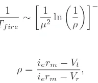
The decay is slower, following an inverse power law, in the case of the Mittag-Leffler function [13]. In both models, the firing rate obtained by incorporating the solutions in a simple passive integrate and fire model, is well approx-imated by [23]
1
Tf ire ∼
1
µ2ln 1
ρ
−κ1
(20)
where
ρ= ierm−Vt
ierm−Vr
, (21)
Vtis the threshold potential for the cell to fire and Vr is
the reset potential after firing. Positive solutions for the firing rate occur for 0< ρ≤1. The anomalous diffusion does not affect the threshold current for nerve cell firing in this model but it does impact on firing rates.
The fractional electro-diffusion models considered in this letter offer new cable equations for spiny neurons where the spines trap and release diffusing molecules re-sulting in anomalously slow diffusion. The additional scaling exponent parameters appearing in temporal op-erators in these equations enable predictions that cannot be obtained from the standard cable equation with ex-isting parameters adjusted to accommodate spines. The linear fractional cable models, which both predict similar qualitative behaviours, could be calibrated and validated through electrophysiological experiments. From Eq.(18), or Eq.(19), withV0= 0, the parametersrm, µ, κcould be
[image:4.595.390.486.409.491.2]ie < 0. Assuming standard values for cm, and κ = γ
in steady state, rL(γ) could be obtained from steady
state voltage attenuation measurements using simulta-neous patch-pipette recordings [31] from the soma and the apical dendrite of a pyramidal neuron. The model prediction for the different arrival times at the soma of dendritic postsynaptic potentials as a function of spine density could be investigated qualitatively through mea-surements of the time course of potentials at the soma in response to currents applied in apical and basal trees, where spine densities are different.
This research was supported by the Australian Com-monwealth Government ARC Discovery Grants Scheme and NIH grants from NIMH and NIDCD, USA.
∗ Electronic address:
B.Henry@unsw.edu.au † Electronic address:
t.langlands@unsw.edu.au ‡ Electronic address:
susan.wearne@mssm.edu;
Computa-tional Neurobiology and Imaging Center.
[1] I. Segev and M. London, Science290, 744 (2000).
[2] W. Rall, Exp. Neurol.1, 491 (1959).
[3] W. Rall, in Handbook of Physiology: The Nervous Sys-tem, edited by R. Poeter (American Physiological Soci-ety, Bethesda, Md, 1977), vol. 1, pp. 39–97, chapter 3.
[4] N. Qian and T. J. Sejnowski, Biol. Cybern.62, 1 (1989).
[5] A. Matus and G. M. Shepherd, Neuron27, 431 (2000).
[6] E. A. Nimchinsky, B.L. Sabatini, and K. Svoboda, Annu. Rev. Physiol.64, 313 (2002).
[7] J. Bourne and K. M. Harris, Curr. Opin. Neurobiol.17, 381 (2007).
[8] G. J. Stuart and B. Sakmann, Letters to Nature367, 69 (1994).
[9] C. Koch,Biophysics of Computation, Information Pro-cessing in Single Neurons, Computational Neuroscience (Oxford University Press, New York, 1999).
[10] S. M. Baer and J. Rinzel, J. Neurophysiol.65, 874 (1991).
[11] F. Santamaria, S. Wils, E. De Schutter, and G. J. Au-gustine, Neuron52, 635 (2006).
[12] K. G. Wang, Phys. Rev. A45, 833 (1992).
[13] R. Metzler and J. Klafter, Phys. Rep.339, 1 (2000).
[14] H. Scher and E. Montroll, Phys. Rev. B.12, 2455 (1975).
[15] M. Saxton, Biophys. J.81, 2226 (2001).
[16] E. Lutz, Physical Review E64, 051106 (2001).
[17] R. Metzler, J. Klafter, and I. M. Sokolov, Phys. Rev. E 58, 1621 (1998).
[18] E. Barkai, R. Metzler, and J. Klafter, Phys. Rev. E61, 132 (2000).
[19] E. Heinsalu, M. Patriarca, I. Goychuk, and P. H¨anggi, Phys. Rev. Lett99, 120602 (2007).
[20] H. C. Tuckwell,Introduction to Theoretical Neurobiology, vol. 1 (Cambridge University Press, Sydney, 1988).
[21] I. M. Sokolov, A. Blumen, and J. Klafter, Physica A302, 268 (2001).
[22] I. M. Sokolov, Phys. Rev. E63, 056111 (2001).
[23] T. A.M. Langlands, B. I. Henry, and S. L. Wearne, in preparation.
[24] B. I. Henry, T. A.M. Langlands, and S. L. Wearne, Phys. Rev. E74, 031116 (2006).
[25] H. M. Srivastava, K. C. Gupta, and S. P. Goyal,The H-Functions of One and Two Variables with Applications (South Asian Publishers Pvt Ltd, New Delhi, 1982).
[26] J. J.B. Jack and S.J. Redman, J. Physiol. 215, 283 (1971).
[27] B. Jacobs, L. Driscoll, and M. Schall, J. Comp. Neurol. 386, 661 (1997).
[28] H. Duan, S. L. Wearne, A. B. Rocher, A. Macedo, J. Mor-rison, and P. R. Hof, Cerebral Cortex19, 950 (2003).
[29] M. Suetsugu and P. Mehraein, Acta Neuropathol50, 207 (1980).
[30] I. Podlubny, Fractional Differential Equations, vol. 198 of Mathematics in Science and Engineering (Academic Press, New York and London, 1999).