Rochester Institute of Technology
RIT Scholar Works
Theses Thesis/Dissertation Collections
11-2016
Detection in Aerial Images Using Spatial
Transformer Networks
Daniel Chianucci [email protected]
Follow this and additional works at:http://scholarworks.rit.edu/theses
This Thesis is brought to you for free and open access by the Thesis/Dissertation Collections at RIT Scholar Works. It has been accepted for inclusion in Theses by an authorized administrator of RIT Scholar Works. For more information, please [email protected].
Recommended Citation
Detection in Aerial Images Using Spatial
Transformer Networks
Detection in Aerial Images Using Spatial
Transformer Networks
DANIEL CHIANUCCI
November 2016
A Thesis Submitted In Partial Fulfillment
Of the Requirement for the Degree of Master of Science
In
Computer Engineering
i
Detection in Aerial Images Using Spatial
Transformer Networks
DANIEL CHIANUCCI
Committee Approval:
_____________________________________________Date:______________ Dr. Andreas Savakis
Primary Advisor – R.I.T. Dept. of Computer Engineering
_____________________________________________Date:______________ Dr. John Kerekes
Committee Member – R.I.T. Center for Imaging Science
_____________________________________________Date:______________ Dr. Dhireesha Kudithipudi
ii
Dedication
iii
Acknowledgments
I would like to thank my advisor Dr. Savakis, for his advice and guidance during the
development and experimentation of this thesis. I also would like to thank my committee
members Dr. Kerekes and Dr. Kudithipudi. Finally I like to thank my peers in the
Computer Vision Lab Peter Muller, Bret Minnehan, and Sriram Kumar who provided
iv
Abstract
Many tasks in the field of computer vision rely on an underlying change detection
algorithm in images or video sequences. Although much research has focused on change
detection in consumer images, there is little work related to change detection on aerial
imagery, where individual images are recorded from aerial platforms over time.
This thesis presents two deep learning approaches for detection in aerial images. Both
systems leverage Spatial Transformer Networks (STN) that identify the coordinate
transformation for their localization capabilities. The first approach is based on a
semi-supervised approach which learns to locate changes within a difference image. The
second is a fully-supervised approach which learns to locate and discriminate relevant
targets. The supervised approach is shown to locate nearly 78% of positive samples with
an Intersection Over Union (IOU) criterion of over 0.5, and nearly 94% of positive
v
Table of Contents
Dedication ...ii
Acknowledgments... iii
Abstract ... iv
Table of Contents ... v
List of Figures ... vii
List of Tables ... viii
Introduction ... 1
Chapter 1. Motivation ... 1
1.1 Thesis Contribution ... 2
1.2 Document Structure ... 3
1.3 Background ... 5
Chapter 2. Change Detection in Consumer Data ... 5
2.1 Change Detection in Aerial Images ... 7
2.2 Deep Learning ... 11
2.3 Spatial Transformer Networks ... 14
2.4 Preliminary Experiments ... 18
Chapter 3. Difference of Reconstructions ... 18
3.1 Difference of Encodings ... 19
3.2 Temporal Feedback ... 21
3.3 Semi-Supervised Approach ... 23
Chapter 4. Methodology ... 23
4.1 Network Architecture ... 23
4.1.1 Network Training ... 25
4.1.2 Sliding Window and Post Processing ... 26
4.1.3 Results ... 28
4.2 Dataset ... 29
vi
Energy Thresholding ... 34 4.2.3
System Results ... 37 4.2.4
Discussion... 39 4.3
Fixed Scale Parameter ... 39 4.3.1
Dataset Complexity and Overfitting ... 41 4.3.2
Semi-Supervised vs Unsupervised ... 41 4.3.3
System Window Overlap ... 42 4.3.4
Real World Viability... 42 4.3.5
Fully Supervised Approach ... 43 Chapter 5.
Methodology ... 43 5.1
Network Architecture ... 44 5.1.1
Training ... 46 5.1.2
Post processing ... 47 5.1.3
Supervised Results ... 48 5.2
WPAFB Dataset ... 48 5.2.1
Localization Results ... 50 5.2.2
Network Weights ... 55 5.2.3
Detection Results ... 59 5.2.4
System Results ... 63 5.2.5
Discussion... 67 5.3
Fixed Scale vs. Free Scale ... 67 5.3.1
Low Resolution Targets ... 68 5.3.2
System Performance ... 68 5.3.3
Conclusions ... 70 Chapter 6.
Concluding Remarks... 70 6.1
Future Works ... 71 6.2
Bibliography ... 73
vii
List of Figures
Figure 1: Activation Functions ... 13
Figure 2: Application of a Spatial Transformer Sampling Grid ... 15
Figure 3: Autoencoder Difference of Encodings. ... 20
Figure 4: Temporal Feedback Mechanism. ... 21
Figure 5: Semi-supervised Network Architecture. ... 24
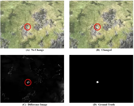
Figure 6: AICD Scene 94 - Viewpoint 0 With Changed Area Circled ... 31
Figure 7: Localization Network IOU Example - ... 32
Figure 8: Qualitative Unsupervised Network Predictions ... 33
Figure 9: Prediction Truth Scenarios ... 34
Figure 10: Unsupervised Energy Based Detection ROC ... 35
Figure 11: Semi-Supervised Energy-Based Detection Precision vs. Recall ... 36
Figure 12: Semi-Supervised System Miss Rate vs FPPI ... 39
Figure 13: Semi-Supervised System Example Predictions ... 40
Figure 14: Supervised Network Architecture ... 45
Figure 15: Full WPAFB Dataset Scene ... 49
Figure 16: Localization and Detection Examples for Free-Scale Network ... 51
Figure 17: Localization and Detection Examples for Fixed-Scale Network... 52
Figure 18: Correct Detections with Low IOU ... 55
Figure 19: First Convolution Layer Weights ... 56
Figure 20: First Dense Localization Layer Weights ... 57
Figure 21: First Dense Layer Detector Weights ... 58
Figure 22: Training Loss History ... 59
Figure 23: Supervised Detector Receiver Operating Characteristics ... 60
Figure 24: Precision vs Recall Curve ... 62
Figure 25: Supervised System Log-Log Miss Rate vs. FPPI on the First K-fold split ... 64
Figure 26: Supervised System Predictions Using Detection Threshold α = 0.8 ... 65
viii
List of Tables
Table 1: Semi-supervised Localization Network Average IOU Results ... 33
Table 2: Unsupervised Area Under Curve and mean Average Precision ... 36
Table 3: Detailed Energy Based Detection Characteristics (min IOU=0.5) ... 37
Table 4: Fixed Scale Network Average IOU Localization Results ... 53
Table 5: Free-Scale Network Average IOU Localization Results ... 53
Table 6: Fixed Scale Network K-Fold Localization Results ... 54
Table 7: Supervised Detector ROC Areas ... 60
Table 8: Detailed Network Test Results For Split 1 (min IOU=0.5) ... 61
1
Introduction
Chapter 1.
Change detection, as the name suggests, is the task of finding differences between a set of
images or across video frames. Many tasks in the field of computer vision rely on an
effective underlying change detection algorithm. For instance, motion detection and
object tracking rely on a change detection algorithm to determine where to focus
attention. Surveillance systems such as Closed-circuit Television (CCTV), and
Unmanned Aerial Systems (UAS) generate huge amounts of data. Without automated
change detection, the task of analyzing each image frame would become unmanageable.
Although change detection seems like a simple challenge, an algorithm can be easily
confused by many sources of background noise. Illumination differences, camera
movement, animated backgrounds, and even compression artifacts can all affect an
algorithms performance. Simple methods, such as difference thresholding can be used
[1]; however such methods generally perform poorly in all but the most ideal scenarios.
In order to robustly detect changes in real world images, more advanced methods must be
employed.
Motivation
1.1
Exploitation of aerial images, especially Wide Area Motion Imagery (WAMI) is
important for military applications, as can be seen by the number of related challenges set
by the United States Air Force Research Labs (AFRL) [2]. In fact, the AFRL listed Wide
2 doctrine [3]. With the changing nature of interactions between adversaries, it is
important that armed and security forces are able to keep an eye on large theaters, while
at the same time having the ability to focus on smaller areas of interest.
Many studies have focused on finding a robust algorithm for change detection in
consumer imagery. Benchmark datasets and leaderboards such as ChangeDetection.net
(CDNET) [2] ease the process of creating and evaluating new algorithms, and also help
immensely with making comparisons to other’s results. However, these benchmarks and
datasets aren’t applicable to wide area coverage. While current datasets focus on high
resolution images where the main topic is the target in question, wide area motion images
are very low resolution, and interesting objects fill only a minute portion of the scene.
Wide Area generally means that the images cover an area greater than 50 square miles
and so it is infeasible for a human analyst to reliably extract the needed information from
a stream of such images. Given the sheer size of WAMI images, the number of pixels is
unmanageable for algorithms developed for consumer applications. This fact has led to
the research and development of techniques adapted towards image processing in WAMI
data. Besides the number of pixels, such research has to deal with other challenges
presented by WAMI data. Small object signatures, as well as low object signal to noise
ratios (SNRs) mean that simple detection algorithms are not sufficient.
Thesis Contribution
1.2
The primary contribution of this thesis is the introduction of two aerial change detection
3 network that are able to learn how to parameterize an image transformation which is
beneficial to a given training objective. They have been shown to excel in fine grained
classification tasks [4][5], but have not been used in the context of change detection or
explicit localization. Rather than using the spatial transformer to find an area which best
differentiates class, it is used to learn the bounding box of a target.
Two approaches are explored; the first is a semi-supervised change detection method
which attempts to find an area of maximal change in a difference image. Given that no
explicit labels are used for training, this method is unable to determine the relevance of a
change, and instead relies on heuristics to reject false positives. A second fully
supervised methodology is employed in order to allow the network to learn the structure
of specific targets. Rather than finding changes directly from a difference image, this
methodology requires a set of registered images and compares the predictions from each.
Both networks are used in a sliding window based approach in order to make multiple
detections per image.
Document Structure
1.3
Following this introduction chapter, Chapter 2 presents a review of previous works.
First, an overview of the state of change detection in consumer data is given. This field
has a number of standardized benchmarks and datasets, and it is relatively
straightforward to compare methodologies. Next, an overview of change detection
techniques for aerial images is presented. This field of change detection is much more
diverse than that of consumer data, and there is no standard benchmark for comparisons.
4 Finally, the chapter concludes with an overview of Spatial Transformer Networks which
are used extensively in this thesis. Chapter 3 provides a narrative of experimental work
which was done prior to the final focus of change detection in aerial imagery. These
experiments were focused on finding a method of robust change detection in consumer
data using autoencoder features. When these features didn’t perform as well as expected,
they provided valuable lessons as the focus was changed to spatial transformer networks
and aerial imagery. Moving forward, Chapter 4 goes into detail about the
semi-supervised aerial change detection method that was explored. First the methodology is
described, including the neural network architecture, the training procedure, and the
post-processing steps. Results are presented, with an overview of the dataset, as well as
qualitative and quantitative test outcomes. Finally, a discussion of interesting phenomena,
shortcomings, and challenges is given. Chapter 5 follows the same structure as Chapter
4, but describes methods, evaluation, results and discussion for the fully supervised
methodology. Finally, Chapter 6 gives concluding remarks, and a statement about
5
Background
Chapter 2.
Change detection is fundamental to many computer vision tasks such as tracking, medical
diagnosis, and surveillance. Although there have been many studies which introduce new
and efficient methods of change detection, most are designed to work with full motion
video taken from ground level cameras. These sequences tend to have a very high spatial
resolution, and so do not directly correlate with those taken from an aerial source.
Although research for this thesis began in the field of change detection in consumer data
sequences, it eventually transitioned to the task of finding changes between a set of two
still images taken from an aerial vantage point. Aerial images present a large number of
challenges including camera motion, large shadows, and extremely small targets to name
a few. The data driven method of deep learning will be used to train a neural network to
locate change targets within large aerial images.
Change Detection in Consumer Data
2.1
Change detection in consumer data is a well-researched topic, and as such has the benefit
of associated standardized benchmarks and datasets. This standardization made the field
an ideal starting point for the research in this thesis.
A broad overview of multiple change detection algorithms is provided in [1]. The
simplest algorithms consist of thresholding a difference image. A difference image as a
map of pixel differences generated using a pixel-wise distance measure between two
6 they suffer from poor performance in real world images. These simple methods are
unable to differentiate between relevant changes, such as those caused by a moving
person, or from irrelevant changes such as those caused by a rustling tree or shadows.
This lack of performance in real life scenarios motivated the development of more robust
methodologies, however, without a standard dataset, these methods were difficult to
compare. As such, the changedetection.net (CDNET) dataset was created in order to
simplify the process of benchmarking the latest advances in change detection [6].
Most approaches submitted for the CDNET dataset ranking build a background model
which is used as a reference for change detection. A popular model choice is to use one
or more probability distributions to represent the likelihood that a pixel value will occur
in an area. However, simple distributions such as those used in Gaussian Mixture Models
[7] and Region-based Mixture of Gaussians [8] do not perform as well as newer methods.
The next step in improving distribution based methods was to utilize models for both
background and foreground. Methods such as Flux Tensor with Split Gaussian Model
(FTSG) [9] and Sharable Model [10] generate such models and take temporal, in addition
to spatial, regions into account. These additions place the two methods towards the top
of the CDNET submission rankings, however higher performing methods do exist.
The two current state of the art methodologies are Pixel-based Adaptive Word Consensus
Segmenter (PAWCS) [11] and Self-Balanced Sensitivity Segmenter (SuBSENSE) [12].
These methods are extremely similar in that they do away with the Gaussian models and
7 Pattern (LBSP) descriptors. A feedback loop is used to adjust both the background
model as well as the comparison threshold according to a stability metric attributed to
each pixel. Stochastic updates are incorporated to prevent the model from becoming
stale.
Finally, the top ranked method, termed In Unity There Is Strength or IUTIS, is an
aggregate of other submitted methods [13]. It uses genetic programming to learn a fusion
strategy to aggregate other methodologies’ results.
One common aspect the majority of the approaches submitted to CDNET share is that
they use engineered features and statistical methods.
Change Detection in Aerial Images
2.2
Due to a lack of a standardized dataset and challenges, the work done in the field of aerial
image change detection is less focused on benchmark data. The large number of image
modalities, scales, and spectral characteristics makes it difficult to compare approaches.
In addition to simple RGB images which is the dominant mode for consumer data, aerial
data also comes in forms such as Wide Area Motion Imagery (WAMI), Synthetic
Aperture Radar (SAR), Panchromatic, and Multispectral. Each of these modalities comes
with its own set of benefits and challenges which must be dealt with. That being said, this
section presents a selection of works which directly relate to change detection in aerial
8 Change detection from aerial images started in the 1960’s when Rosenfeld proposed a
variety of correlation metrics to measure the similarity between image features [14].
Early research into change detection came to the realization that not only do geometric
and radiometric distortions need to be accounted for, but also that changes would need to
be categorized to reject irrelevant variation such as those caused by clouds or shadows.
These challenges led to the discovery of symbolic techniques, in the 1970’s and 1980’s,
which emphasized the detection of changes based on the shapes, sizes, and radiometric
properties contained within the images [15]–[17]. These techniques generally use a
segmentation technique to separate the image into discrete areas, which can then be
classified based on shape, texture, or spectral features. In particular, [18] uses edge
detection, and Hough line transforms to detect changes based on straight line matching.
This approach is particularly well suited for updating urban Geographic Information
System (GIS) data due to the often grid like city plans.
With advancements in remote sensing technologies and the introduction of Wide Area
Surveillance (WAS) new techniques were developed for detecting man made changes in
in larger scenes. In [19], a man made change detection technique is described which
involves modeling the spectral and size changes which can be expected during facility
construction. These changes are harder to model than naturally occurring changes due to
the fact that they aren’t as predictable as changes observed for crops and other vegetation
over time.
In the early 2000’s an uptick in research involving Artificial Neural Networks (ANN) is
9 techniques, these studies use very small neural networks consisting of only a few layers,
each using less than 15 neuron units. In [20] Principal Component Analysis (PCA) was
used to generate features from multispectral pixel data. These features were then used to
train and evaluate a three layer ANN to classify features into land use classes. These
predicted classes were then used to determine if a change had occurred in land use
between two images. Similarly, [21] uses a three layer neural network to predict an after
image from a before image, and vice versa. A set of heuristics is then used to determine
if the prediction is unusual.
Approaching the late 2000’s, a type of neural network called a Self-Organizing Feature
Map (SOFM) began to be used. An SOFM is a nonlinear generalization of PCA [22],
and is used to learn a low dimensional representation of the input space in an
unsupervised manner. Both [23] and [24] use an SOFM network to classify areas into
changed and not changed regions, however where the first classifies entire segments at a
time, the second classifies individual pixels.
A more recent method which uses an SOFM was introduced in [25]. This method detects
changes to building structures in high resolution RGB images. First, a histogram of
illumination invariant features is used to train an SVM for building detection. Then, an
SOFM based active contour model is used for boundary extraction. The extracted
boundaries can then be used to compare areas between images.
A non-machine-learning approach was introduced in [26], which uses optical flow to
detect changes between a set of aerial images. This paper introduced the simulated
10 optical flow on a set of registered images in order to remove changes caused by simple
parallax effects.
A statistical tile based methods was introduced in [27], which split an image into equally
sized tiles and performed change detection at the tile level rather than the pixel level.
This approach takes tiles from a set of registered images and determines a tiles change
potential based on a set of complimentary metrics. The difference of spectral distribution
means, or mean-shift, is used to quantify large scale changes within a tile, while the
greatest distance between a pixel and the distribution mean, or and outlier-distance, is
used to quantify small scale changes. Combining these metrics allows tiles which contain
large or small scale changes to be detected.
Similarly, [28] introduces a graph theoretic approach to detect tile level changes between
two registered images. With this approach, a weighted adjacency matrix is calculated for
each tile, along with the Standard Deviation of Edge Weights edges (SDEL). A metric
coined the Normalized Edge Volume (NEV) is used to measure the spectral variability
between two registered tiles. Large scale changes within a tile correspond with large
NEV values, whereas small scale changes correspond with large SDEL value. Although
both tile based methods were shown to work well in variety of situations, the resolution
of the output change map is limited by the size of the tiles.
Deep learning has been used recently to detect changes between a set of SAR images. In
[29], a two input deep neural network is trained to produce a change map directly. This
11 image. This method however was only shown to work well for large change targets such
as coastlines, and farmland fields.
Finally, recent research by Kitware and AFRL[30], has found that change detection in
WAMI images can be greatly enhanced by applying the differencing to a detection
response map rather than to the raw image pixels. By running a Histogram of Oriented
Gradients (HOG) based vehicle detection Support Vector Machine (SVM), this paper is
able to create a heat map of sort denoting the likelihood that a vehicle is present. When
two of these maps are registered and differenced, the pixels with large differences are
taken to be potential changes. This process significantly reduces the number of residual
bright areas caused by illumination and parallax differences. This method of detecting
changes between detection maps rather than raw images was a motivation for the
supervised detection methodology presented in this thesis.
Deep Learning
2.3
Deep learning is a term which encompasses neural networks containing many layers.
These networks aim to emulate the connections in the human brain in order to learn a rich
and robust set of features. Deep learning approaches have been successfully used in
many machine learning applications, especially in the area of computer vision. Many
variants of deep networks exist, each with its own benefits and detractors.
The basic concept of a neural network can be represented by a graph of compute nodes.
Each node takes a set of inputs and provides a single output. Although individually, each
12 continuous function [31]. This sounds like an end all solution; however the difficulty
comes in training the network to perform as desired.
Training a neural network consists of multiple steps. First, network architecture must be
developed, or borrowed. Basic architectures consist of an input layer, a series of internal
hidden layers and finally an output layer. Each layer is generally followed by a nonlinear
function called nonlinearity or an activation function. Early deep neural networks
consisted solely of dense layers which perform a dot-product of the weights and the input
[32]. Common activation functions included sigmoid and hyperbolic tangent functions.
However, since each neuron in a dense layer connects to each and every neuron in the
previous layer, the number of connection weights which must be learned increases at a
rapid pace. This motivated the introduction of convolutional layers in 1998 which allow
weights to be shared across spatial extents [33]. Convolutional networks have been
shown to excel in many computer vision tasks due to their ability to preserve the 2D
structure of an image [34]–[36]. Recently, activation functions being used have shifted
towards Rectified Linear Units (ReLU) rather than sigmoidal forms. These nonlinearities
take the form of a simple max operation as seen in Figure 1, and don’t suffer from issues
such as vanishing or exploding gradients seen in other nonlinearities. One issue they do
have however is that non active units contribute nothing to the gradient, and as such
become permanently inactive. A simple solution is to introduce a small slope for
negative samples to make a “Leaky ReLU”.
Once the architecture has been selected, the feature learning can begin. A sample is fed
13 the network onto the output. An objective function such as mean square error or
categorical crossentropy then calculates an error metric between the prediction and the
ground truth. This error is then passed back through the network as a series of gradients
in a process called back propagation in order to update the weights.
𝑆𝑖𝑔𝑚𝑜𝑖𝑑 = 1 1 + 𝑒−𝑥
𝑡𝑎𝑛ℎ 𝐿𝑒𝑎𝑘𝑦 𝑅𝑒𝐿𝑈
= max (𝑚 ⋅ 𝑥, 𝑥)
Figure 1: Activation Functions
Although Neural Networks have proven to be very successful they require a large number
of labeled samples to train. One network architecture which aims to solve this is the
autoencoder.
In the simplest form, an autoencoder consists of a neural network appended with its own
inverse. The network is then trained to reconstruct the input. In essence, an autoencoder
is a neural network which aims to approximate the identity function. Because the identity
function isn’t very interesting in and of itself, constraints are imposed on the network in
order to force it to learn interesting structures. For instance, common constraints include
making the middle layer much smaller than the input, or enforcing sparsity on the middle
14 space. As with self-organizing feature maps, autoencoders can be thought of as a
nonlinear generalization of PCA [38]. A second approach termed a denoising
autoencoder involves introducing noise to the input, and train the network to reproduce a
clean output [39]. This forces the autoencoder to learn only salient features in the
presence of noise.
Spatial Transformer Networks
2.4
A new class of neural networks deemed Spatial Transformer Networks (STN) has
recently been introduced [4]. As the name suggests, these networks learn to parameterize
a spatial transformation on an image or feature map in order to focus on pertinent areas.
The main building block of a spatial transformer network is the Spatial Transformer
layer. This specialized layer does not contain any weights, and as such does not learn on
its own. Rather it applies a differentiable transformation given by a parameterized input
onto an input feature map. Because the transformation is differentiable, gradients are
able to flow through this layer during backpropagation in order to update the weights of
both the transformation parameter input, as well as the feature map input. If the
transformation parameters are provided by a neural network, as intended, then the
backpropagation allows the transformation to be learned.
Although the transformation may take any form as long as it remains differentiable, the
authors focus on pointwise affine transformations, given by the form shown in (1), where
(𝑥𝑖, 𝑦𝑖) is a normalized coordinate on the input space, (𝑥𝑖𝑡, 𝑦𝑖𝑡) is a normailized coordinate
15 [𝑥𝑦𝑖
𝑖] = 𝑇𝜃(
𝑥𝑖𝑡 𝑦𝑖𝑡 1
) = [𝜃11 𝜃12 𝜃13 𝜃21 𝜃22 𝜃23] (
𝑥𝑖𝑡 𝑦𝑖𝑡 1
) (1)
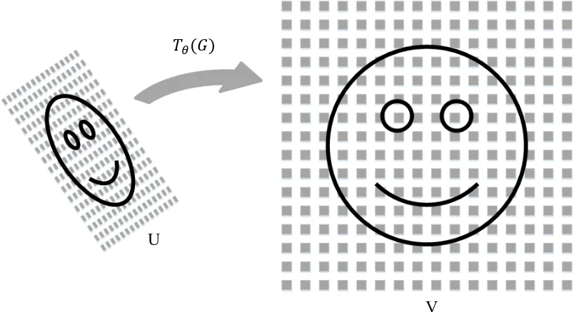
By applying such a transformation to a regular grid 𝐺 = {(𝑥𝑖𝑡, 𝑦𝑖𝑡)}, consisting of all target pixel coordinates, an output feature map consisting of input space sampling points
is generated. The input image is then sampled and interpolated using the generated
[image:26.612.100.502.298.517.2]points, resulting in a transformed image as shown in Figure 2.
Figure 2: Application of a Spatial Transformer Sampling Grid
Each coordinate (𝑥𝑖, 𝑦𝑖) generated by the sampling grid represents the location in the source image, U, where a sampling kernel is applied to get the pixel value for the output,
V. A bilinear sampling kernel is shown in (2), where 𝑉𝑖𝑐 is the output value for pixel 𝑖 on V
U
16 channel 𝑐. Similarly, 𝑈𝑛𝑚𝑐 denotes the input pixel at coordinate (𝑛, 𝑚). The two 𝑚𝑎𝑥
functions determine the relative weight for each pixel to obtain the bilinear interpolation.
𝑉𝑖𝑐 = ∑ ∑ 𝑈𝑛𝑚𝑐 ⋅ max(0,1 − |𝑥
𝑖 − 𝑚|) ⋅ 𝑊
𝑚 𝐻
𝑛
max(0,1 − |𝑦𝑖− 𝑛|) ∀𝑖∀𝑐 (2)
For back propagation to occur, partial derivatives must be calculated. For the bilinear
kernel shown in (2), the partial derivatives can be calculated as follows.
𝛿𝑉𝑖𝑐
𝛿𝑈𝑛𝑚𝑐 = ∑ ∑ max(0,1 − |𝑥𝑖− 𝑚|) ⋅
𝑊
𝑚 𝐻
𝑛
max(0,1 − |𝑦𝑖− 𝑛|) (3)
𝛿𝑉𝑖𝑐 𝛿𝑥𝑖
= ∑ ∑ 𝑈𝑛𝑚𝑐 ⋅ max(0,1 − |𝑦 𝑖 − 𝑛|) 𝑊
𝑚 𝐻
𝑛
⋅ 𝑠𝑖𝑔𝑛(max(0,1 − |𝑥𝑖− 𝑚|)) (4)
The partial derivative shown in (3), allows gradients to flow backwards from the output
to the input feature map. The derivative shown in (4) on the other hand allows the
gradients to flow from the output to the sampling coordinates, and in turn the
transformation parameters and localization network. Note that the partial derivative with
respect to 𝑦𝑖 follows a similar equation to (4).
Spatial transformer networks have been shown to perform extremely well in
classification tasks [4], [5]. In these tasks the localization portion of the STN will
inherently learn to focus onto the portion of the feature map which is best able to
discriminate between classes. The ability to learn the size and shape of the important
image regions would seem to be a perfect fit for the task of changed target detection;
17 With that being said, this thesis proposes a new method to train an STN in order to
parameterize the bounding box of changed targets within aerial images. First, a
semi-supervised approach to finding changes within a difference image is presented. This
method receives no information on the structure of relevant targets during training. In
order to better predict only relevant targets, a supervised approach is also introduced.
This method integrates a detection network with the semi-supervised architecture which
allows structure to be learned.
18
Preliminary Experiments
Chapter 3.
Although this thesis eventually settled on change detection in aerial images, the initial
experiments that were run were more geared towards detecting changes in full motion
consumer videos. This section serves as a narrative of the process that was followed in
order to end at the new focus.
The desired approach was leveraging deep learning features. Because learned features
are robust to various sources of noise, it follows that they would excel in tasks, such as
change detection, where environmental noise is expected. However, because real world
change detection scenarios don’t have human labelled ground truths, deep learning is
severely limited. This presents an opportunity for unsupervised learning with
autoencoders.
Difference of Reconstructions
3.1
The first approach considered was to train an autoencoder, and use its reconstructions to
generate a difference image. The thought was that since autoencoders tend to retain only
major aspects of an input, differencing the reconstruction rather than the original images
would result in a difference image with only major changes. In the case of change
detection, where one does not need nor want to detect inconsequential changes, this loss
of small details could be a benefit.
Multiple models of autoencoder were tested by trial and error. The final model consisted
19 pooling layer. The first convolutional layer consisted of 32 7x7 filters, the second was 16
5x5 filters, and the final convolution was 16 3x3 filters. The decoder portion of the
network was a linear inverse of the encoder described.
A deep convolutional autoencoder model was trained on 32x32 patches from the CDNET
video sequences. The training objective was set to minimize the mean square error
between the input and output images, the reconstructions still contained remnants of the
inconsequential changes. If the network was instead trained to reconstruct a clean
background, defined as the pixel wise median of the previous temporal window, the
network would simply overfit. The bias of the final layer learned to emulate the mean of
the entire sequence, while the weights stop contributing to the output. If the bias was
then constrained, the network simply reverts to modeling the input image including
irrelevant changes.
Difference of Encodings
3.2
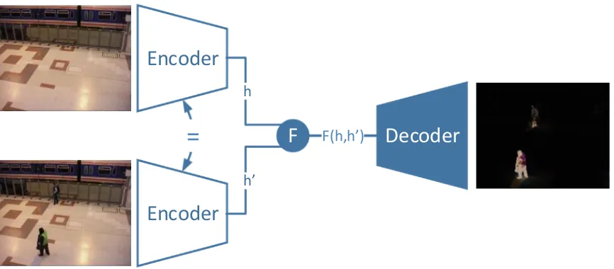
It was then hypothesized that if the difference was taken at the feature level, then the
resulting encoding would decode back into a clean difference image similar to what is
seen in Figure 3. First an autoencoder was trained using the same method as the
“Difference of Reconstructions” autoencoder described above. The encoder and decoder
portions were then split apart. A changed image and a clean image were fed through the
encoder portion to generate two encodings represented as h and h’. A function, F, is
applied to h and h’ which generates a third encoding. This third encoding is sent through
20
Encoder
Decoder
Encoder
=
F
F(h,h)h
[image:31.612.92.525.74.264.2]h
Figure 3: Autoencoder Difference of Encodings.
Both clean and changed images are fed through the encoder portion of the autoencoder. A function F is applied to the hidden representations h and h’. The result is decoded using the decoder portion of the network, thus resulting in a difference image
Because the encoded features are an abstract representation, there is no established
method to compare two encodings. Therefore, in an attempt to generate a clean difference
image, both the difference and absolute difference were tested. However, the resulting
reconstructions tended to be blurry and contain bright halos. These reconstructions were
thresholded and cleaned using morphological operations; however evaluation proved that
similar results could be obtained by simply applying the same morphological operations
to a standard difference image. This finding ultimately led to seeking alternate
21
Temporal Feedback
3.3
Image
Representation Change Mask
Classification Stability Update Rate
Distance Threshold
[image:32.612.124.487.149.316.2]Background Model
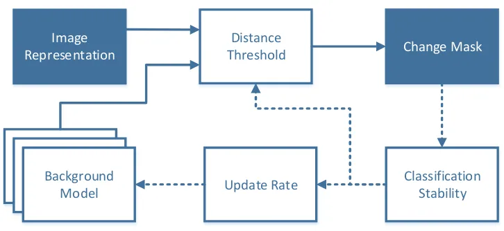
Figure 4: Temporal Feedback Mechanism.
At each time step the autoencoder hidden representation of an image is input, and a change mask is output. A stability metric is used to update the distance thresholds, and background update rate.
Autoencoder features were next considered in a different setting. Looking into the
feedback based approaches of SuBSENSE and PAWCS [11], [12], it can be seen that the
results are dependent on the robustness of the underlying features being used. A similar
feedback mechanism shown in Figure 4 was developed to test the feasibility of
autoencoder features in comparison to the LBSP features used in [11] and [12].
Although autoencoder features showed promise in theory, in practice they did not work
as well as expected. The LBSP features and feedback used by PAWCS and SuBSENSE
produced cleaner results, and were much less computationally expensive. Where LBSP
descriptors can be calculated using simple comparison operations, autoencoder features
22 descriptors are still more efficient in the fact that distance comparison requires only XOR
operations, whereas floating point math is required with autoencoder features.
Because of the computational load accompanying autoencoder features, even if detection
performance was on par with the state of the art, the low computational efficiency would
rule them undesirable for this application. Although there were high expectations for the
use of autoencoders in change detection, they tended to not perform as well as desired.
For this reason, the focus was altered towards using spatial transformers and aerial
23
Semi-Supervised Approach
Chapter 4.
In this chapter a semi-supervised approach to change detection in aerial images is
introduced. This method aims to find unstructured changes between two images. This is
accomplished using a Spatial Transformer, which is trained to find an area of maximal
change in a difference image.
Methodology
4.1
A Spatial Transformer Network was utilized to localize changes transforming its input
image so the output viewport contained maximal change. In this case, maximum change
is defined as maximum Euclidean distance between the original and changed images.
The assumption that significant changes will result in bright areas in the difference image
was made, however this heuristic doesn’t hold in all cases. It is additionally expected
that a system trained using this methodology will only work correctly on images which
are taken from similar sensors and altitudes.
The trained network is used with a sliding window based approach in order to detect
multiple changes in a single image. A heuristic based approach is used for post
processing in order to reject false positives and merge similar predictions.
Network Architecture 4.1.1
Since change is defined as maximum Euclidean distance between input samples, it is
24 generated by taking the pixel-wise Euclidean distance between the clean and changed
RGB images. This results in a greyscale image in which significant changes tend to
appear as structured bright patches, whereas illumination differences tend to appear as
smooth gradients. The task of the neural network is to help distinguish which of these
[image:35.612.143.487.240.502.2]areas contain actual changes, and which are insignificant.
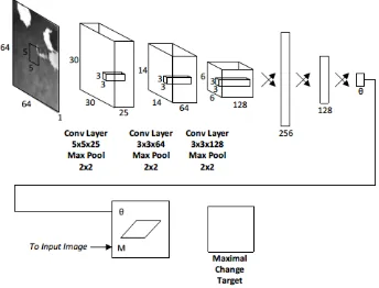
Figure 5: Semi-supervised Network Architecture.
The network architecture, displayed in Figure 5, consists of three convolution-pool layers
followed by three dense layers and finally a spatial transformer. From first to last, the
convolution layers consist of 25, 64, and 128 filters respectively. All convolution layers
25 is followed by a 2x2 max-pooling layer. The final pooling layer is followed by three
consecutive dense layers consisting of 256, 128, and 2 units respectively. The first two
dense layers utilize the same leaky ReLU nonlinearity, while the final dense layer,
labeled 𝜃, parameterizes the spatial transform and as such is left linear. Finally, the
spatial transformer applies the 𝜃 transform to the input difference image, and outputs the
result.
The transformation parameter 𝜃, consists of two outputs corresponding to translation in the x and y directions. The scale parameter of the affine transformation is fixed at 50%,
which approximately matches the size of the desired targets. For reasons conferred in the
discussion, the fixed scale is necessary when using this methodology.
This particular network architecture was found through trial and error by starting with a
very small network and growing it both in width and depth until the network began to
overfit. At this point it was shrunk slightly to remove the overfitting. Both 5x5 and 3x3
filters were experimented with in the convolutional layers, as well as using a standard
ReLU nonlinearity rather than the leaky ReLU. The final architecture represents the best
of the tested architectures after training.
Network Training 4.1.2
Training data was generated from the Aerial Image Change Detection dataset described
below. The 500 generated difference images were split into 80% training and 20%
holdout sets, leaving 400 training images and 100 test images. Positive sample patches
26 windows from the center of the desired structure. For each of the images, 10 patches were
extracted using random offsets, resulting in 4000 positive training samples and 1000 test
samples.
Only positive samples are used during training in an attempt to get the network to overfit
to the desired structures. Although the network doesn’t receive explicit labels during
training, the fact that only positive samples are used requires there to be an implicit label
associated with each patch. This method is thus not fully unsupervised, and so the term
semi-supervised is more accurate.
The loss function is defined as the mean square error between the predicted patch, and a
maximally changed patch, which in the case of a scaled difference image is a fully
saturated greyscale patch. Stochastic gradient descent with Nesterov momentum is used
during the backpropagation pass to update the network weights.
Sliding Window and Post Processing 4.1.3
In order to detect multiple changes per image, a sliding window is employed. A 64x64
window is moved across the image, and a single location prediction is generated for each
window position. Because the localization network is able to further narrow the location
to a 32x32 box within a given window, it is unnecessary to visit every possible window
location, and a strided approach was taken instead. A sequence of post-processing filters
27 The first filter is based on the observation that the network tends to predict a translation
of 0 if there are no structures present. As such, (5) shows that the first filter takes the set
of all location predictions,𝑃, and retains only the predictions which have a maximum
translation of at least 𝛼. The new set of filtered predictions is labelled 𝑃𝑡. Maximum
translation, 𝒎(𝑃), is defined in (6) as the maximum magnitude of the x and y axis translations, where 𝑇𝑥 and 𝑇𝑦 are the translation in the x and y directions. It must be
noted that using the 𝛼 threshold is only useful when operating the sliding window where
it is guaranteed that at least one window will contain the object off center. Otherwise,
windows which happen to contain a centered object will be rejected.
𝑃𝑡 = {𝑃(𝑖) | 𝒎(𝑃(𝑖)) ≥ 𝛼 ∀𝑖} (5)
𝒎(𝑃) = 𝒎𝒂𝒙(|𝑇𝑥|, |𝑇𝑦|) (6)
The next step is to filter out patches of flat texture which have low energy using (7). This
filter takes the set of translation filtered predictions, 𝑃𝑡, as described above and retains
only those with an energy above a threshold 𝛿. The remaining predictions are placed in the set labeled 𝑃𝑒. The energy function, 𝒆(𝑃), shown in (8) defines the energy of
prediction 𝑃 to be the mean squared error between 𝑝 and 𝜇, where 𝑝 is the set of pixels in
28 𝑃𝑒 = {𝑃𝑡(𝑖) | 𝒆(𝑃𝑡(𝑖)) ≥ 𝛿 ∀𝑖} (7)
𝒆(𝑃) = 𝒎𝒆𝒂𝒏 ((𝑃(𝑖𝑗)− 𝜇)2) (8)
The final filtering stage uses Algorithm 1 to combine predictions for which the overlap
ratio is greater than 𝛽, and to remove any predictions for which fewer than 𝛾 original predictions agreed upon. The final set of predictions is taken to be the set of bounding
boxes left over after post-processing.
Results
4.2
In the experimental setting, Python 3 was used as the programming language for all tasks.
A combination of Nolearn [40], Lasagne [41], and Theano[42] API’s were used to model
the neural network. Theano is a tensor based computing API which allows for automatic
differentiation, as well as GPU acceleration of tensor operations. Lasagne is a library
which defines many common neural network layer types in terms of Theano tensors.
Finally, Nolearn is a wrapper around Lasagne which makes it compatible with the
29
Algorithm 1: Merge and Overlap Filter
Both training and testing were performed using an Intel Core i5 6200U processor in
addition to an Nvidia GeForce 940M GPU. The Neural Network Analysis and training
were performed with a parallel batch size of 10 64x64 image patches. The Sliding
window was performed sequentially using no GPU resources. Training the network took
roughly 30 seconds per epoch, and took around 37 epochs to fully converge. This results
in just under 30 minutes hours of training with the 4000 training patches. Running the
analysis takes about 2 minutes 10 seconds to make predictions for the 1000 test patches.
Dataset 4.2.1
The Aerial Image Change Detection (AICD) dataset was used for the semi-supervised
30 training [26]. This dataset consists of 100 simulated scenes each captured from 5
viewpoints giving a total of 500 samples. For every sample, the dataset provides the
clean image, the image with a change, and the ground truth. Figure 6 shows an example
for a single sample viewpoint. Although, each scene has both shadowed and
un-shadowed variants, this experiment, only used the un-shadowed versions. The small number
of images contained in this dataset makes it very important to keep the network
complexity in check. With such a small dataset, too large of a network would not be able
to fully train.
Localization Results 4.2.2
To characterize the localization ability of the network, all samples in the holdout set were
passed through the network to collect predicted class and locations. Because no attempt is
made to determine the relevancy of the predicted area, the prediction is irrelevant for
negative samples. However if the sample is positive, then it is desired that the predicted
area match the target area. Therefore, the Intersection Over Union (IOU) ratios between
the predicted bounding box and ground truth bounding box were recorded for all positive
samples. The IOU is a measurement which characterizes how well two areas overlap.
As the name suggests, it is calculated by dividing the area of the bounding boxes
geometric intersection by the area of their geometric union. In cases where multiple
31 As an example, Figure 7shows a patch with multiple ground truth objects represented as
circles; only the maximum IOU between the predicted square, and green circle is
recorded. The localization performance was then calculated as the average IOU over all
positive samples, along with the percentage of prediction areas which matched the
ground truth.
(A) No Change (B) Changed
[image:42.612.80.534.86.445.2](C) Difference Image (D) Ground Truth
32
Figure 7: Localization Network IOU Example - The maximum IOU is recorded between the predicted square and green circle
The average IOU of all predictions with their respective ground truths is shown in Table
1. The final column shows the percentage of predictions which match the ground truth
location with an IOU greater than the given threshold. An IOU of 0.5 is the standard
used in consumer image detection challenges such as the Pascal Visual Object Challenge
[43], however in these challenges the target boxes tend to contain many thousands of
pixels, and as such small deviations in bounding boxes don’t effect the overall IOU
significantly. In contrast, if a 32x32 px bounding box with an IOU of 0.5 is offset by
only 4 pixels in both directions, then the IOU can decrease to 0.3. As such multiple IOU
thresholds, including 0.1, 0.3, and 0.5, are tested.
The average IOU of 0.57 is lower than expected, but can be explained by the
non-structural learning targets. Because the localization target is to simply find the “most
changed” area, there is no way for it to determine which changed area it is desirable to
33
Table 1: Semi-supervised Localization Network Average IOU Results
Match
Threshold Match %
0.1 99.4% 0.3 87.0% 0.5 62.1%
Avg IOU
0.57 ±0.2
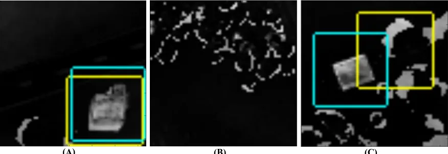
As an example, Figure 8 shows three qualitative examples of network predictions. In
(A), the network has correctly identified the desired target changed area. Note however
that there is very little background noise. In (B), the network has found an arbitrary
location, but the energy threshold has determined that there is no object present. Finally,
(C) shows that the network has trouble with background noise which is of similar size
and shape to the desired structure. The network has performed the given task of finding
the significantly changed area; however in this case, the given task doesn’t match with
what is actually desired. Cases similar to this can be expected to decrease the average
IOU as well as the percentage of matched predictions.
(A) (B) (C)
Figure 8: Qualitative Unsupervised Network Predictions - Yellow is the predicted box, blue is the ground truth box
(A) The network has correctly localized the object of interest in a low noise environment (B) The network has correctly determined that no object of interest is present
[image:44.612.91.529.480.631.2]34
Energy Thresholding 4.2.3
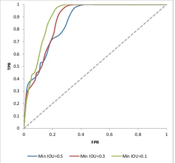
In order to measure the ability of the energy function to reject false positives, a Receiver
Operating Characteristics (ROC) curve was generated by varying the 𝛿 threshold. This curve plots the true positive rate against the false positive rate in order to visualize the
tradeoff between finding all positive samples and finding no negative samples. Because
only the predicted patch is seen by the energy function, the ground truth was taken to be
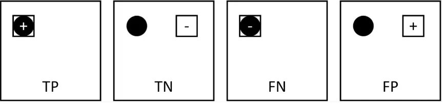
whatever was present within the given predicted area, as shown in Figure 9. Note that
although all patches contain a ground truth object, the test result is determined solely by
what is contained inside the predicted area. For a predicted area to be considered as
containing a ground truth object, it must overlap with the object with an IOU above a
[image:45.612.91.523.407.509.2]given threshold.
Figure 9: Prediction Truth Scenarios – The circle is the ground truth, the square is the predicted area, the sign is the class prediction, and the text at the bottom indicates the test result
The ROC curves shown in Figure 10 show that although the energy based relevancy
measure isn’t ideal, it performs significantly better than random given the locations
provided by the network. When the network is used in the system, the translation of the
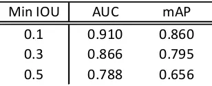
35 In order to quantify the ROC performance as a scalar value, the Area Under the Curve
(AUC) is calculated. Table 2 shows a summary of the calculated AUC scores for the
tested ground truth IOU thresholds. With a minimum IOU of 0.5, the AUC of 0.788
shows that there is room for improvement, however given that the relevancy measure
[image:46.612.126.488.253.590.2]does not take the target’s structure into account it is about as good as can be expected.
Figure 10: Unsupervised Energy Based Detection ROC
The Precision vs. Recall curve shown in Figure 11 was also generated for the different
IOU thresholds. As can be seen, the semi-supervised approach loses precision steadily as
0 0.1 0.2 0.3 0.4 0.5 0.6 0.7 0.8 0.9 1
0 0.2 0.4 0.6 0.8 1
TPR
FPR
36 recall is increased. The mean Average Precision (mAP) for the network is listed
alongside the AUC in Table 2. It can be seen that the minimum IOU threshold has a
large impact on the precision of the network due to the fact that the average IOU of the
[image:47.612.141.474.195.530.2]location predictions is close to the threshold to begin with.
Figure 11: Semi-Supervised Energy-Based Detection Precision vs. Recall
Table 2: Unsupervised Area Under Curve and mean Average Precision
Min IOU AUC mAP 0.1 0.910 0.860 0.3 0.866 0.795 0.5 0.788 0.656 0
0.1 0.2 0.3 0.4 0.5 0.6 0.7 0.8 0.9 1
0 0.2 0.4 0.6 0.8 1
Pr
e
ci
si
o
n
Recall
[image:47.612.230.384.613.676.2]37 Table 3 gives the detailed truth counts for the semi-supervised network when the
localization IOU threshold is set at 0.5. Metrics given include False Positive Rate (FPR),
True Positive Rate (TPR), Precision (Pr), Specificity (Sp), F-Measure, and Percent
[image:48.612.100.516.246.572.2]Wrong Classification (PWC). See Appendix I for metric definitions.
Table 3: Detailed Energy Based Detection Characteristics (min IOU=0.5)
δ TP TN FP FN FPR TPR Pr Sp F-meas PWC
0.100 14 1379 0 607 0.00 0.02 1.00 1.00 0.04 30.4% 0.095 33 1377 2 588 0.00 0.05 0.94 1.00 0.10 29.5% 0.090 57 1373 6 564 0.00 0.09 0.90 1.00 0.17 28.5% 0.085 86 1369 10 535 0.01 0.14 0.90 0.99 0.24 27.3% 0.080 120 1365 14 501 0.01 0.19 0.90 0.99 0.32 25.8% 0.075 180 1355 24 441 0.02 0.29 0.88 0.98 0.44 23.3% 0.070 216 1344 35 405 0.03 0.35 0.86 0.97 0.50 22.0% 0.065 236 1321 58 385 0.04 0.38 0.80 0.96 0.52 22.2% 0.060 257 1267 112 364 0.08 0.41 0.70 0.92 0.52 23.8% 0.055 283 1232 147 338 0.11 0.46 0.67 0.89 0.54 24.3% 0.050 327 1220 159 294 0.12 0.53 0.67 0.88 0.59 22.7% 0.045 333 1195 184 288 0.13 0.54 0.64 0.87 0.59 23.6% 0.040 367 1162 217 254 0.16 0.59 0.63 0.84 0.61 23.6% 0.035 441 1115 264 180 0.19 0.71 0.63 0.81 0.67 22.2% 0.030 468 1038 341 153 0.25 0.75 0.58 0.75 0.65 24.7% 0.025 507 983 396 114 0.29 0.82 0.56 0.71 0.67 25.5% 0.020 559 943 436 62 0.32 0.90 0.56 0.68 0.69 24.9% 0.015 604 890 489 17 0.35 0.97 0.55 0.65 0.70 25.3% 0.010 621 795 584 0 0.42 1.00 0.52 0.58 0.68 29.2% 0.005 621 703 676 0 0.49 1.00 0.48 0.51 0.65 33.8% 0.000 621 0 1379 0 1.00 1.00 0.31 0.00 0.47 69.0%
System Results 4.2.4
When running the system as a whole there is an ambiguity as to what constitutes a true
positive. Because an overlapping window is used, multiple positive predictions may map
38 multiple ground truth locations. To handle this ambiguity, the Pascal Visual Object
Challenge (VOC) method of only accepting a single prediction per ground truth is used.
If multiple predictions match with a single ground truth, only the first is considered a true
positive, while the rest are considered false positives. In this case a match is defined as
two boxes with an IOU ratio greater than 0.5. More specifically, the truth counts are
defined as follows:
TP – Number of ground truths which match at least one prediction
FN – Number of ground truths which don’t match any predictions
FP – Number of predictions, which don’t match an available ground truth
TN – Total Number of Predictions – (TP+FP+FN)
To measure the system wide performance the post processing sequence was run using
various combinations of α, β, γ, and δ in order to generate Miss Rate vs False Positives
Per Image (FPPI) curve. The patch agreement threshold 𝛾 was test with values of 1 and
2. It was found that at 𝛾 = 1, the system benefitted from a higher energy threshold 0f 0.02, while at 𝛾 = 2, a lower energy threshold of 0.01 worked slightly better.
Figure 12 shows the Miss Rate curve for four sets of parameters. The systems using two
overlapping windows run slightly better than the systems with four overlaps due to the
smaller possible number of negative samples which must be rejected. Even still, the high
FPPI shows that the localization network selects irrelevant changes too often, and the
energy and translation heuristics are not a strong enough method to reject the large
39 Figure 13 shows example results for four scenes using parameters 𝛼 = 0.4, 𝛽 = 0.5, 𝛾 =
[image:50.612.161.452.196.463.2]2, and 𝛿 = 0.01. A common aspect of all four images is the number of false positives which pass the energy and translation heuristics.
Figure 12: Semi-Supervised System Miss Rate vs FPPI
Discussion
4.3
Fixed Scale Parameter 4.3.1
When running the semi-supervised network, it became apparent that if the affine
transformation scale parameter was left as a trainable parameter, then the network would
simply learn to zoom onto a single bright pixel in the input patch. Given the definition
0.01 0.1 1
1 10 100 1000
M
iss
R
ate
FPPI
40 that change is represented by relative brightness in a difference image, this was the most
convenient way for the network to find the maximal area of change, however it is
obviously not the desired operation.
(A) (B)
[image:51.612.162.498.194.504.2](C) (D)
Figure 13: Semi-Supervised System Example Predictions
(A) The target has been found, in addition to false positives (B) The target was missed, with few false positives
(C-D) The target is missed with many false positives
One potential method to counteract this without imposing a fixed scale would be to apply
a penalty to predictions with small scales, however since the general size of the targets
was known, it was easier to tune the scale parameter directly than to tune a penalty
41
Dataset Complexity and Overfitting 4.3.2
The AICD is very small dataset in terms of deep learning applications. The fact that the
simulated images lack much complexity that would be present in a real image, along with
the fact that there are only 500 scenes, means that anything but the simplest of networks
would over fit.
Even with positive samples only, the network didn’t quite operate as desired. Rather than
overfitting to positive samples, it seems to find the largest bright area with little to no
indication that it prefers the desired target over other differences. The simulated nature
of the dataset may play a role in this outcome, as the shadows tend to have very sharp
edges and lack subtleties found in real images. However this cannot be tested for using
only the AICD dataset.
Semi-Supervised vs Unsupervised 4.3.3
As noted, although this methodology doesn’t give the network explicitly labelled data,
the fact that it only trains with positive samples implies that there must be an implicit
label for each sample. Due to the fact that the network is trained with only positive
samples, by definition it isn’t unsupervised, however because no labels are used during
training it isn’t fully supervised either. Since the network doesn’t completely lie in either
42
System Window Overlap 4.3.4
When qualitatively assessing the semi-supervised network, it became apparent that it was
able to parameterize transformations with larger translation components than the
supervised counterpart. Because it proposes areas closer to the edges of the input patch,
the overlapping window didn’t need to be as dense as with the supervised network. This
can be seen by the fact that the best performing version of the system uses only two
overlaps vs the four used by the supervised system.
Real World Viability 4.3.5
Although the semi-supervised method was an interesting experiment it needs additional
training on large scale datasets before it can mature into a viable change detection
solution. The network is able to locate changes within an image, but without any
reference to what constitutes a relevant change, the network will not be able to determine
this distinction on its own.
This can be seen by the large number of predicted locations which correspond to an
irrelevant change. Since relevant changes tend to be greatly outnumbered by irrelevant
changes, such as illumination differences, a method of determining a change’s relevancy
is needed. Given that fact that implicit labels are needed anyways, it may be more
43
Fully Supervised Approach
Chapter 5.
In this section a fully supervised method is presented which builds on the
semi-supervised approach described in the previous chapter. Rather than trying to find an
arbitrary area of maximum change, this methodology is paired with a binary classifier in
order to detect specific targets. This not only increases localization performance, but also
removes the need for the heuristics and replaces them with an explicit detection network.
Rather than finding changes directly, this methodology instead detects specific targets. In
order to detect changes, a set of registered images is required. If a target is detected at the
same position in both images, then no change has occurred, however if the target is only
present in a single image, then a change has occurred.
Methodology
5.1
The supervised approach aims to combine the tasks of localization and detection by using
a Spatial Transformer Network. Rather than attempting to find an arbitrary area of
maximal change, this network is trained to find specific targets in a grayscale aerial
image. A neural network binary classifier is appended to the transformation, and used as
a detector. The entire network is trained end to end using multi task regression.
The trained network is then integrated with a sliding window similar to that used with the
semi-supervised approach. Rather than heuristically rejecting false positives, the trained
44 As with the semi-supervised methodology, it is expected that a system which uses this
methodology will only work on images which contain similar targets taken from
comparable altitudes using the same type of sensors. If these limitations are not
conformed to, then the target signatures will be too dissimilar for the detection network to
reliably find. In order to make the methodology generalizable, a dataset containing the
desired target types and altitudes must be used for training.
Network Architecture 5.1.1
The network shown in Figure 14 is based on the network used in the semi-supervised
method with three exceptions. First, the scale parameter of the affine transformation does
not need to be fixed at a predefined value. Second, the localization target is now a
specific structure rather than an arbitrary change. And third, a second spatial transformer
and detection network have been added.
The first spatial transformer branch performs the transformation directly to the 64x64
input patch and outputs a zoomed in image patch labeled “localization output”. This
branch is trained to reconstruct the 32x32 patch centered on the structure of interest as