Rochester Institute of Technology
RIT Scholar Works
Theses Thesis/Dissertation Collections
8-2017
Three-dimensional Image Processing of Identifying
Toner Particle Centroids
Di Bai
Follow this and additional works at:http://scholarworks.rit.edu/theses
This Thesis is brought to you for free and open access by the Thesis/Dissertation Collections at RIT Scholar Works. It has been accepted for inclusion in Theses by an authorized administrator of RIT Scholar Works. For more information, please [email protected].
Recommended Citation
Three-dimensional Image Processing of Identifying Toner Particle Centroids
by Di Bai
A Thesis submitted in partial fulfillment of the requirements for the degree of
Master of Science in Print Media in the School of Media Sciences
in the College of Imaging Arts and Sciences of the Rochester Institute of Technology
August 2017
Primary Thesis Advisor: Dr. Shu Chang
ii
School of Media Sciences Rochester Institute of Technology
Rochester, New York
Certificate of Approval
[Three-dimensional Image Processing of Identifying Toner Particle Centroids]
This is to certify that the Master’s Thesis of Di Bai has been approved by the Thesis Committee as satisfactory for the Thesis requirement for the Master of Science in Print Media degree at the
convocation of August 2017 Thesis Committee:
Dr. Shu Chang, Primary Thesis Advisor
Dr. Elena Fedorovskaya, Secondary Thesis Advisor
Christine Heusner, Graduate Program Director
iii
Acknowledgments
I would like to express my gratitude to my thesis committee Dr. Shu Chang,
Dr. Elena Fedorovskaya, and Prof. Christine Heusner for their invaluable expertise,
aspiring guidance, and friendly support during my thesis work. I would also like to thank
Dr. Howard Mizes for his professional guidance and valuable input on the 3D imaging
algorithm implementing. I also would like to express my warm thanks to Professor
Robert J. Eller and Dr. Patricia Sorce for their support and guidance on editing my thesis.
I am truly grateful to them for sharing their truthful and illuminating views on issues
iv
Table of Contents
Acknowledgments ... iii
List of Tables ... vii
List of Figures ... viii
Abstract ... x
Chapter 1: Introduction and Statement of the Problem ... 1
Reason for Interest in the Study ... 4
Chapter 2: Theoretical Basis ... 5
Image Preparation for Three-dimensional Convolution ... 5
Median Filter ... 5
Binary Image Conversion ... 7
Fill Function ... 8
Three-dimensional Kernel and Convolution ... 9
Chapter 3: Literature Review ... 14
Particle Centroids Detection in Colloidal System ... 15
Particle Centroids Detection in Powder System ... 21
Three-dimensional Image Analysis: Kernel and Convolution ... 26
v
Chapter 4: Research Objectives ... 29
Chapter 5: Methodology ... 30
Three-dimensional Particle Sighting Approach ... 31
Image Enhancement ... 32
Three-dimensional Convolution ... 33
Locating Particle Centroids ... 34
The Ground Truth ... 34
Accuracy Assessment ... 35
Chapter 6: Results ... 36
Three-dimensional Particle Sighting Results ... 36
Results of Image Enhancement ... 37
Results from the Three-dimensional Convolution Process ... 38
Centroids of Particles ... 39
Result of Accuracy Assessment ... 40
Efficiency of the Three-dimensional Particle Sighting Method ... 42
Chapter 7: Discussion ... 43
Existence of Dark Pixels Inside Images of Solid Toner Particles ... 43
Locating Particle Centroids in a Sea of 1s ... 44
Mismatch of 3D Particle Sighting and Frame-by-Frame Results ... 45
Chapter 8: Conclusions ... 47
Agenda for Future Research ... 49
vi
Appendix A: 3D Particle Sighting Matlab Code ... A
Appendix B: Particle Detection Matlab Code ... B
vii List of Tables
viii List of Figures
Figure 1. Example of applying a 3x3 median filter to replace one pixel in an image. ... 6
Figure 2. Example of using a median filter on an original gray scale image ... 7
Figure 3. Example of binary conversion of a gray scale frame image ... 7
Figure 4. Example of the fill function applied on a binary frame image. ... 8
Figure 5. Example of how convolution works in two dimensions. ... 10
Figure 6. Example of a 3D kernel and a 3D image matrix.. ... 11
Figure 7. Result from convolution of the kernel matrix with the image matrix.. ... 12
Figure 8. Example of a one-dimensional Gaussian kernel function created in Matlab.. .. 13
Figure 9. Illustration of point spread function (PSF) in an optical microscopy. ... 18
Figure 10. Example of a region of interest for imaging under the confocal microscopy. 22 Figure 11. Example of locating X and Y coordinates of a particle’s centroid. ... 23
Figure 12. Example of sampling a “particle of interest” at different Z values in two image frames. ... 24
Figure 13. Flowchart of the Three-dimensional particle sighting process. ... 31
Figure 14. Flowchart of the image processing procedure. ... 32
Figure 15. Flowchart for generating a convolution matrix from a 3D image matrix and a 3D Gaussian kernel. ... 33
ix
Figure 17. Ground truth: the centroids of particles detected by Patil with (x, y, z)
coordinates. ... 35
Figure 18. Process of image enhancement from an original RGB image (depicted in (a)) to
a filled binary image (shown in (e)).. ... 37
Figure 19. Plot of particle centroids detected by the 3D particle sighting method. ... 40
Figure 20. Agreement between 3D particle sighting results and frame-by-frame results. 41
Figure 21. Visualization of mismatched paired centroids. ... 42
Figure 22. Example of a dark region inside a CLSM image of solid toner particles. ... 44
Figure 23. Visualization of mismatched paired centroids. ... 46
x Abstract
Powder-based 3D printed products are composed of fine particles. The structure
formed by the particles in the powder is expected to affect the performance of the final
products constructed from them (Finney, 1970; Dinsmore, 2001; Chang, 2015; Patil,
2015). A prior study done by Patil (2015) demonstrated a method for determining the
centroids and radii of spherical particles and consequently reconstructed the structure
formed by the particles. Patil’s method used a Confocal Laser Scanning Microscope to
capture a stack of cross-sections of fluorescent toner particles and Matlab image analysis
tools to determine the particle centroid positions and radii. Patil identified each particle
centroid’s XY coordinates and particle radius layer by layer, called “frame-by-frame”
method; where the Z-position of the particle centroid was estimated by comparing the
radius change at different layers. This thesis extends Patil’s work by automatically
locating the particle centroids in 3D space.
The researcher built an algorithm, named the “3D particle sighting method,” for
processing the same stacks of two-dimensional images that Patil used. The algorithm at
first, created a three-dimensional image matrix and then processed it by convolving with
a 3D kernel to locate local maxima, which pinpointed the centroid locations of the
xi
convolution operation automatically located the particle centroids. By treating Patil’s
results as the ground truth, the results revealed that the average delta distance between the
particle centroids identified through Patil’s method and the automated method was
1.02µm ± 0.93µm. Since the diameter of the particles is around 10µm, this error is small
compared to the size of the particles, and the results of the 3D particle sighting method
are acceptable. In addition, this automated method need 1/5 of the processing time
1 Chapter 1
Introduction and Statement of the Problem
Powder systems, a bulk solid composed of a large number of fine particles that
may flow freely when shaken or tilted, are widely used in industry (Duran, 2012; Fayed,
2013; Holdich, 2002; Rhodes, 1990). However, as the researcher’s literature reviews
show, there is only a limited amount of research analyzing the spatial distribution of
particles in these structures by using Confocal Laser Scanning Microscopy (CLSM)
(Bromley, 2012; Chang, 2014; Chang, 2015; Patil, 2015). In Confocal Laser Scanning
Microscopy, an optical microscope is used to capture cross-sections of samples that are
transparent or fluorescent (Bromley and Hopkinson, 2002; Van & Wiltzius, 1995). It has
been used for characterizations and three-dimensional visualizations of micron-size
particles in diluted colloidal systems (Baumgartl & Bechinger, 2005; Besseling et al.,
2015; Bromley & Hopkinson, 2002; Crocker & Grier, 1996; Dinsmore et al., 2001;
Habdas & Weeks, 2002; Jenkins and Egelhaaf, 2008; Pawley, 2010; Prasad,
Semwogerere & Weeks, 2007; Schall et al., 2004; Semwogerere & Weeks, 2005; Van &
Wiltzius, 1995). Colloidal systems, as opposed to powder systems, are generally wet
systems in which at least one component phase has a length scale between a nanometer
and a micrometer (Duran, 2012; Jenkins, 2006). It has been shown that the positions of
2
reviewed in Chapter 3)and reconstructed into a 3D volume (Crocker & Grier, 1996;
Habdas & Weeks, 2002; Jenkins & Egelhaaf, 2008; Semwogerere & Weeks, 2005).
Images captured from CLSM have also been used to visualize and characterize
powder systems in recent studies (Chang, 2014; Chang, 2015; Patil, 2015). Patil (2015)
conducted experiments to visualize the microstructures manifested by
electro-photographic toner powders. In his research, Patil used the “frame-by-frame” method,
which also provides the ground truth for this thesis, to identify the centroids of toner
particles in a stack of 2D cross sectional images captured by a confocal microscope. The
particle centroids’ XY coordinates and particles’ radii were identified within each
layer-frame, and the Z-position of each particle was assessed by comparing the radius change
of the particle obtained at different frames. Patil’s method is time consuming since the
researcher needs to examine each frame manually. For example, the processing time for
locating 30 particles in a 256x256x192 matrix using the frame-by-frame method is
between 150 and 250 minutes.
In this research, the objective is to create an automated method to detect the
centroids of particles in an efficient way, using a 3D convolution algorithm. The 3D
convolution and kernel are widely used in image processing techniques, such as center
detection, edge detection, feature extraction, and noise reduction (Hopf & Ertl, 1999;
Kim & Han, 2001; Suzuki et al., 2006; Kim & Casper, 2013; Xu, Yang, & Yu, 2013).
This is realized through a convolution operation between a kernel and an image. In image
processing, a kernel is a matrix, which could be as small as a 3x3 matrix and convolution
3
the kernel (Brown et al., 1950; Jain, A. K., 1989; Kenneth, 1996). The 3D convolution is
utilized in fields including human action recognition (Xu, Yang & Yu, 2013), shape
feature extraction (Suzuki et al., 2006; Suzuki & Yaginuma, 2007), solid texture analysis
(Hopf & Ertl, 1999), and vector distance field (Fournier, 2011). As a commonly known
technique, 3D convolution has been used in applied research, for example, detecting corn
flour starch suspended in immersion oil (Bromley, 2002). However, the researcher was
unable to find prior research applying 3D convolution algorithms to locate the centroids
of dry powder particles (without immersion oil). This thesis will explore its use in dry
toner particle centroids detection. This research is important to address in the burgeoning
field of 3D printing, where the analysis of solid microstructures becomes necessary for
predicting macrostructural performance of 3D printed objects. The 3D particle sighting
method has the potential to enable significant progress in the understanding of
structure-property relationships for powder materials in 3D printing. By understanding the
microstructure of the powder materials, researchers could improve their ability to choose
proper materials for 3D printing. Furthermore, being able to visualize the microstructure
of powder material particles could help material scientists to compare the properties of
different kinds of materials. Both the 3D printing industry and the materials science
discipline would benefit from these improvements.
In this thesis, the researcher developed an automated method for locating the
centroids of electro-photographic toner particles by using a 3D convolution algorithm.
Images from Patil’s (2015) research were processed using the proposed methodology.
4
ground truth of Patil’s locations. This research is significant because it automates and
significantly accelerates the process of detecting the centroids of particles compared to
the previous frame-by-frame method with the acceptable accuracy.
Reason for Interest in the Study
The researcher’s interest in this subject was born when he worked with Patil on
Dr. Shu Chang’s research team. Patil generated the frame-by-frame method to detect the
centroids of toner particles by using a confocal microscope. This method had to be done
using each layer-frame and was time consuming. The researcher wanted to find a new,
efficient method to detect the centers automatically and accurately. Dr. Chang and Dr.
Howard Mizes enlightened the researcher about the idea of using 2D or 3D convolution
algorithms, because they were powerful tools used in different image processing
techniques. This led to the following research question: Can we apply a convolution
algorithm to toner particle detection? That was the start of this research.
The researcher’s primary thesis advisor, Dr. Shu Chang, has a strong background
in material science, and the researcher’s secondary advisor, Dr. Elena Fedorovskaya, has
expertise in computer science. They opened the researcher’s eyes and intensified his
interest in 3D image processing for toner particle center detection. From them, the
researcher was infected with a desire to improve the existing method (Patil’s
frame-by-frame method) based on a stack of 2D CLSM images. As a result, the researcher was
motivated to develop an automated and accurate method to locate the centers of toner
5 Chapter 2 Theoretical Basis
In this chapter, the researcher will define image filtering, three-dimensional
kernel, and convolution. The researcher will also discuss the principle of using a 3D
convolution to locate centers of particles. The researcher will discuss image preparation
for 3D convolution and utilization of 3D kernels and implementing 3D convolution to
locate the center of each particle.
Image Preparation for Three-dimensional Convolution
Images were processed using Image Processing Toolbox in the Matlab software
package. Three main functions from this Image Processing Toolbox are used to prepare
images for 3D convolution: a median filter, a binary image conversion, and a fill
function.
Median Filter
Filtering in image processing is a basic function that is used to accomplish tasks,
including noise reduction, interpolation, resampling and so on. Choosing a filter is based
6
mean filter and non-linear filters, such as median filter. The difference between a linear
filter and a non-linear filter is whether its output is a linear or non-linear function of its
input.
The median filter replaces the center value in the window with the median of all
the pixel values in the window (Lim, 1990). An example of median filtering for a single
3x3 window is shown in Figure 1, where a 3x3 median filter is applied to replace one
pixel in an image. In this case, 90 in the center of the 3x3 filter window in Figure 1(a) is
replaced with the median value in the filter window (depicted as 1,2,2,3,4,5,9,18,90),
which is 4. This process is repeated for each pixel in the image to convert the raw image
into a filtered image.
[image:18.612.188.479.364.501.2]
Figure 1. Example of applying a 3x3 median filter to replace one pixel in an image. The pixel, 90 in (a), is replaced by the median value of the pixels in the filter window (1,2,2,3,4,5,9,18,90), which is 4. The resulting window is in (b).
In this research, a median filter is used to remove 'impulse' noise (outlying values), as
illustrated by Figure 1. A median filter has been used to remove satellite dots (impulse
noise) from the images captured by a confocal microscope in previous research (Kenneth,
1996).
7
Figure 2 shows the result of using a median filter to remove satellite dots from an
image of toner particles captured by the confocal microscope used in this research.
[image:19.612.213.442.144.234.2]
Figure 2. Example of using a median filter on an original gray scale image (depicted in (a)). The median filter removes the satellite dots shown as small gray particles against the dark gray background (a) to create the filtered image in (b).
Binary Image Conversion
The binary conversion process transforms gray scale images into binary images as
shown in Figure 3. Figure 3 depicts a frame from a stack of CLSM images of toner
particles in gray scale against a black background after a median filter has been applied to
remove impulse noise (a), and the subsequent image’s conversion into a binary image (b).
The grey level image shown in (a) contains pixel values ranging from 0 to 255. A
threshold is used to convert (a) to (b), so that the pixels in the binary image (b) have only
two intensity values, 0 for black and 1 for white, and are displayed in black and white.
[image:19.612.215.439.536.653.2]
Figure 3. Example of binary conversion of a gray scale frame image (depicted in (a)). When the specified threshold is added, the binary conversion converts the pixel values ranging from 0 to 255 (shown in (a)) to 0 and 1 (shown in (b)).
8
Fill Function
The third step in image processing is to apply a “imfill.m” function to the binary
image obtained by applying the median filter and binary conversion. A “imfill.m”
function fills isolated background regions within an object’s boundaries (Soille, 2003).
The “imfill.m” function used in this thesis with the corresponding parameters is provided
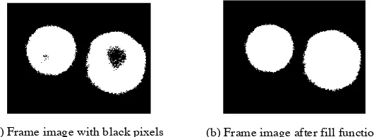
in Appendix A. Figure 4 depicts a part of a frame from a stack of CLSM images of dry
toner particles after applying a median filter and binary conversion showing black pixels
in the white particle areas (a), and the result of applying a fill function to this image (b).
The fill function first defines the boundary of each particle and then fills the region
within the boundary by converting black pixels within the boundary into white pixels.
[image:20.612.198.463.367.464.2]
Figure 4. Example of the fill function applied on a binary frame image (depicted in (a)). Fill function defines the boundary of each particle and then fills the white region within the boundary by converting black pixels (pixel value = 0) into white pixels (pixel value = 1).
After image preparation for 3D convolution is complete, the resulting image has
no noise in the background, and has particles with well-defined boundaries and uniform
pixel values. After image preparation, CLSM frames can be stacked into a 3D matrix and
convolution operation can be applied to accurately locate particle centers.
9 Three-dimensional Kernel and Convolution
In image processing, a kernel is a matrix, which dimensionality can range
between 1-D and N-D. Kernels have been used in fields including human action
recognition (Xu, Yang & Yu, 2013), shape feature extraction (Suzuki et al., 2006; Suzuki
& Yaginuma, 2007), solid texture analysis (Hopf & Ertl, 1999), vector distance field
(Fournier, 2011), and particle center detection (Bromley, 2002). In this thesis, a 3D
kernel will be used to detect the centers of powder particles. When using a kernel to find
the center of a particle, the kernel is convolved with the pixel image. Laplace (1891)
described convolution as a function that is the integral or summation of two component
functions that measures the amount of overlap as one function is shifted over the other. In
this thesis, the images captured by CLSM are first processed by the three steps previously
indicated and then combined into a three-dimensional image matrix. After that, a 3D
convolution is applied.
Mathematically, a 3D convolution can be described by equation 1:
A 𝑖%, 𝑗%, 𝑘% ∗ B 𝑖+, 𝑗+, 𝑘+ = C 𝑖., 𝑗., 𝑘. = 89:1𝐴 𝜏1, 𝜏2, 𝜏3 𝐵[𝑖 − 𝜏1, 𝑗 − 𝜏2, 𝑘 − 𝜏3]
;<=>
?9:1
;@=>
A9:1
;B=> (1)
A 𝑖%, 𝑗%, 𝑘% stands for the pixel value in the 3D image matrix at the location 𝑖%, 𝑗%, 𝑘% ,
where 𝑖%, 𝑗%, 𝑘% designates the location of pixel a in the 3D image matrix. Similarly,
B 𝑖+, 𝑗+, 𝑘+ represents the value of the 3D kernel matrix at the location 𝑖+, 𝑗+, 𝑘+ in the
kernel matrix. C 𝑖., 𝑗., 𝑘. stands for the value of the resulting convolution (C) matrix at
10
The function of a 3D convolution is best understood by starting with a 2D
example. The reader can imagine that kernel matrix “slides” over the image matrix one
unit at a time with the sum of the products of the two matrices as the result. Figure 5
shows the convolution of an image matrix and a kernel at a single coordinate. A 2D 3x3
kernel is designed to produce a maximum value in the convolution matrix at the point
corresponding to the particle center in the original image. Note that here we only consider
one original 2D image or a 2D frame from a stack of images with the fixed Z coordinate.
Each value in the convolution matrix is calculated by summing the products of the image
pixel values and the values in the kernel. In this example, the value of 25 is calculated as
1x2+1x2+1x2+1x2+3x3+1x2+1x2+1x2+1x2. To fill in the remaining cells in the
convolution matrix, the 3x3 kernel must be repositioned to be centered on each of the
[image:22.612.268.479.429.629.2]original image cells.
Figure 5. Example of how convolution works in two dimensions. Each value in the convolution matrix is calculated by summing the products of the 2D image pixel values and the values in the kernel. The complete convolution is achieved by repeating the process until the kernel has passed over every possible pixel of the source matrix.
Kernel
Original image
Product
11
In this case, the result of convolution is a convolution matrix which has a property
that the maximum value of the convolution matrix is located at the center of the matrix if
the size of the kernel is greater than the size of the image matrix. Once the convolution
matrix is rescaled to match the size of the image matrix, the maximum value in the
convolution matrix corresponds to the location of the particle center in the image matrix.
In three dimensions, an analogous example is shown in Figures 6, 7, and 8.
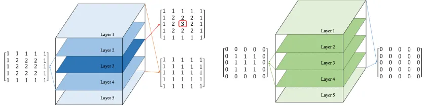
Figure 6 (a) shows a 5x5x5 kernel, which means a 3D matrix with 5 layers and 5x5
matrix in each layer. Notice that the kernel matrix has a single maximum value in the
center with smaller values surrounding it, which is the same as the kernel used in this
research. A 5x5x5 volume of a 3D image is shown in Figure 6 (b). After preparing the
CLSM images, the researcher combined them into a 3D image matrix. This 3D image
matrix is similar to the matrix shown in Figure 6 (b) with particle areas all equal to 1 and
background areas equal to 0.
[image:23.612.121.541.453.558.2]
Figure 6. Example of a 3D kernel and a 3D image matrix. (a) is a 5x5x5 kernel with 3 pixel values ranging from 1 to 3, especially 3 is in the center of the kernel matrix. This kernel matrix is similar to the kernel used in this research. Notice that this kernel has a single maximum value in the center and smaller values surrounding it. (b) is a 5x5x5 volume extracted from an image matrix with pixel values restricted to 0 and 1. This image matrix is similar to the image matrix used in this research with particle area values equal to 1 and background area values equal to 0.
12
When a 3D image matrix is convolved with a 3D kernel, the kernel must be first rotated
twice in three dimensions to correctly align the kernel with the image prior to multiplying
the two matrices. Because the kernel in Figure 6 (a) is symmetrical, the result of this
rotation is not visible to the reader.
The result of convolving the kernel in Figure 6 (a) with the 3D image matrix in
Figure 6 (b) is shown in Figure 7. As the kernel scans through the image area, a 3D
convolution matrix is generated. The resulting matrix is 9x9x9 with the center value 55.
After convolution, we have a single maximum value (55) in the convolution matrix. Once
the convolution matrix is rescaled to match the size of the image matrix, the location of
the maximum value in the convolution matrix corresponds to the location of the particle
center in the image matrix.
[image:24.612.135.508.408.593.2]13
As shown in Figure 7, using a kernel with a single maximum in its center results
in a convolution matrix with a single maximum that corresponds to the location of the
particle center in the image matrix. The researcher used a 3D Gaussian kernel in this
research. Mathematically, a 3D Gaussian kernel can be described by equation 2:
F(E,F,G)= 𝐹E∗ 𝐹F∗ 𝐹G= 12Jexp − E:NO
@
2PO@ ∗ 1
2Jexp − F:NQ @
2PQ@ ∗ 1
2Jexp [− (F:NQ)@
2PQ@ ] (2)
F(E,F,G)stands for the 3D Gaussian kernel, which is the result of multiplying FE,
FF and FG. FE, FF and FG are Gaussian function in X, Y, Z directions. For example, in the
x direction, 𝜇E designates the mean value and 𝜎E represents standard deviation.
As we know each single function, for example, 𝐹E= 12Jexp − E:NO
@
2PO@ , has one single
maximum value in its center. Figure 8 shows a graph of one-dimensional Gaussian kernel
function. Because the maximum value of the one-dimensional Gaussian function is in the
center of the graph, so that the result of multiplication, which is the 3D Gaussian kernel,
[image:25.612.267.381.504.600.2]will have the property that its single maximum value occurs in its centroid.
Figure 8. Example of a one-dimensional Gaussian kernel function created in Matlab. The maximum value of the kernel is in its center.
The researcher used a smooth Gaussian kernel to remove noise and limit the number of
14 Chapter 3 Literature Review
As this thesis is proposing an automated detection of toner particle centroids
based on a stack of 2D CLSM frame images using a 3D convolution method, the
literature review covers previous approaches for detecting particle centroids, especially
the particles that were observed with Confocal Laser Scanning Microscopy (CLSM).
Although in this thesis the researcher detected the centroids of a powder material system
used in electro-photographic digital printing (toner) instead of colloidal particles, CLSM
had been widely used in colloidal system analysis. So, this chapter is organized as
follows:
• The first section: “Particle centroids detection in colloidal system” will review
particle centroids detection in colloidal systems.
• The second section: “Particle centroids detection in powder system” will review
particle centroids detection in powder systems, especially Bromley and
Hopkinson’s (2002) experiment that utilized CLSM to determine the centroid
positions of corn flour starch particles and Patil’s “frame-by-frame method” of
detecting the centroids of toner particles. Deficiencies of the reviewed methods will
15
particle sighting method” will be shown in comparison with the reference
frame-by-frame method.
• The third section: “Three-dimensional image analysis: kernel and convolution” will
review several applications of 3D convolution in image processing for center
detection, edge detection and feature extraction and address the applicability of the
3D convolution approach for the toner particle detection.
Particle Centroids Detection in Colloidal System
Current Confocal Laser Scanning Microscopy (CLSM) techniques have been used
to capture a stack of cross-sectional images of particles (Bromley & Hopkinson, 2002;
Van & Wiltzius, 1995). Once cross-sectional images are captured, image processing tools
are used to locate the centroids of particles three-dimensionally (Besseling et al., 2015;
Bromley & Hopkinson, 2002; Crocker & Grier, 1996; Dinsmore et al., 2001; Habdas &
Weeks, 2002; Jenkins & Egelhaaf, 2008; Pawley, 2010; Prasad, Semwogerere, & Weeks,
2007; Semwogerere & Weeks, 2005; Schall et al., 2004; Van & Wiltzius, 1995).
Confocal microscopy is typically used to visualize micron-sized particles in colloidal
systems where particles are diluted and suspended (Jenkins & Egelhaaf, 2008; Prasad et
al., 2007; Schall et al., 2004). These include colloidal fluids (Frank et al., 2003;
Semwogerere, Morris, & Weeks, 2007), glasses (Isa, Besseling & Poon, 2007; Isa et al.,
2009), and gels (Conrad & Lewis, 2010; Conrad & Jennifer, 2008; Kogan & Solomon
2010). One of the early studies using a confocal microscope to visualize colloids was
16
sample of charged polystyrene latex colloids and found hexagonal gathering of the
spheres. Analyzing microstructure of the system is important to determine the material
properties and performance of the object. Confocal microscopy provides a tool to image
the system, but in order to reconstruct the microstructure and analyze the microstructure
properties of a system, such as packing density, coordination number and nearest
neighbor distance, researchers need to improve visualization based on a stack of frame
images because visualization is one of the means to understand microstructure. Since
microstructure reconstruction and property analysis can be determined by measuring the
centroid coordinates and radii of the particles, developing algorithms to locate the
centroids of particles is a necessary step. Specifically, several algorithms were created to
will be reviewed, namely, Crocker and Grier’s (1996) algorithm, Jenkins and Egelhaaf’s
(2001) algorithm and the Hough Transformation.
Crocker and Grier (1996) implemented a method of locating centroids of colloidal
particles by finding the local brightest pixel in each frame. In practice, they identified a
pixel as a candidate center if all other pixels within a distance were dimmer than it. For
example, they first located the center of one particle (circle) in each frame image, which
is the (X, Y) coordinates of the center. Then they matched up centers in the stack of
images to find the middle frame of the centers of this particle, which was the Z position
of that particle’s centroid. With X and Y coordinates and Z position, the real centroid of
each particle was identified. Two applications using Crocker and Grier’s algorithm to
locate the center of particles are reviewed next.
17
(1996) algorithm to investigate the structure and flow behavior of colloidal gels with
confocal microscopy. The gel they used was composed of coated silica particles with a
diameter of around 824nm. After acquiring image stacks in a high-density sample using
confocal microscopy, they used Crocker and Grier’s algorithms to locate the centroids of
the particles in three dimensions and reconstruct the structure of particles and flow
profiles of colloidal gels.
In the second example, Dinsmore et al. (2001) used Crocker and Grier’s (1996)
algorithms to locate the centroids of poly-methyl methacrylate (PMMA) particles that
were suspended in colloidal solution in three dimensions. They used two solvents,
cycloheptyl bromide (CHB, 97%; Aldrich) and cyclohexyl bromide (CXB, 98%;
Aldrich), that match the refractive index of the particles so that the scanning depth of the
colloids could reach 100 microns under CLSM. Dinsmore et al. (2001) found that using a
solvent that matches the refractive index of the particles would improve the resolution of
the cross-section images. Their method of improvement in the setup can deal with
colloidal particles well; however, the Crocker and Grier’s algorithm has limitations.
There are three limitations in Crocker and Grier’s (1996) algorithm. Firstly, this
algorithm does not include point spread function (PSF). The PSF happens in the imaging
system when researchers visualize spheres under a microscope. The PSF would change
the shape of the sphere to be an elliptical solid along the Z-axis or XY plane of a scan. An
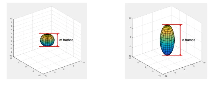
illustration of point spread function is shown in Figure 9. In this figure, a spherical
particle occupying the length of 10 𝜇𝑚, which is corresponding to m number of frames in
18
microscope, where n > m.
[image:30.612.137.509.113.265.2]
(a) Particle occupies 10𝜇𝑚 (m frames) in Z-axis (b) Particle occupies 15𝜇𝑚 (n frames) under confocal microscope
Figure 9. Illustration of point spread function (PSF) in an optical microscopy. Due to PSF in a microscopy, a spherical particle occupying the length of 10μm (m frames) in the Z-axis (depicted in (a)) is shown to occupy the length of 15μm (n frames) under the microscope, which n>m (shown in (b)).
Secondly, even though comparing the pixels with neighboring pixels to locate the
center of the particles is straightforward, for this algorithm to work, the images must have
only one single maximum pixel in the center. This means the method cannot deal with the
case if the pixel values are the same in the particle area. Thirdly, Crocker and Grier’s
method is a two-dimensional based algorithm, which means they had to detect the local
brightest pixel in each frame. Other researchers tried to overcome described limitations.
For example, Jenkins and Egelhaaf (2008) improved the Crocker and Grier’s
(1996) algorithm by adding a refinement step called sphere spread function (SSF), which
was used to overcome the PSF. The SSF refinement is the convolution of sphere function
with the PSF. After SSF refinement, the elliptical solid would be transformed to a sphere
19
Egelhaaf increased the accuracy of the centroids detection of the colloidal particles since
the particles were closer to their real shape. Jenkins and Egelhaaf (2008) also introduced
a second strategy to recover the original shape of the particle by computing
deconvolution of its PSF from the observed particle image under CLSM. Both, the
deconvolution method and the SSF refinement method are aiming to recover the original
shape of the particles. However, the deconvolution algorithm has a limitation that the
deconvolution or refinement result would be significantly affected by the noise in the
image, so it cannot be applied to noisy images.
Jenkins and Egelhaaf (2008) proposed to use a new method called the Hough
Transform (Hough, 1962) to overcome the limitation of Crocker and Grier’s (1996)
method that images must have only one single maximum pixel in the center. The Hough
Transform is widely used for feature extraction in computer vision (Gonzalez, 1992).
This method can be used to detect centers, radii of circles (Gonzalez, 1992) and the
outlines of arbitrary shapes (Ballard, 1981; Duda and Hart, 1972). Specifically, Hough
Transform can be applied to objects with different shapes and is not constrained to an
object with the brightest center. It operates by inverting the parameters of original space
to parameters in the Hough space. For example, a line in Cartesian coordinate system can
be defined as y = ax + b. This can be transformed into a set of two parameters: slope and
intercept, which is (a, b) and in Hough space, which is a new Cartesian system with a axis
and b axis, (a, b) is just a point. Each point in the Hough space corresponds to a line in
the original space. However, the limitation of Hough transform is the difficulty of using it
20
into a set of two parameters: slope and intercept. But in 3D, objects usually need more
than three parameters, and Hough Transform is not efficient in 3D object detection.
Chang et al (2015) used the Hough Transform in their research to identify the particle
centroids and radii in two dimensions frame by frame. They also used a feature from the
Leica Application Suite called the Region of Interest analysis to find the depth (or Z
value) for a particle.
To sum up, CLSM has been used in colloidal systems to capture stacks of
cross-sectional images so that researchers used image processing tools to identify the centroids
of particles. Crocker and Grier’s (1996) algorithm can locate the centroids of particles by
finding the local brightest pixel in each frame of a stack of images. But their algorithm
has apparent limitations: (1) it does not count point spread function, (2) images must have
single maximum pixel in the center, and (3) it’s a 2D based algorithm. The point spread
function can be overcome by SSF refinement or deconvolution process when the images
are not noisy. Another method, the Hough Transform, can solve the second limitation
because it can be applied to objects with different shapes and not constrained to a
maximum center. However, the Hough Transform is difficult to utilize in 3D systems
with over three parameters. So, more research should be conducted to identify a method
to detect centers of particles with the same pixel values in the particle area automatically
in 3D. In this thesis, the researcher generated algorithms for locating centroids of toner
powder particles instead of a colloidal system particles. In the next section of this
literature review, a previously published powder particle centroids detection algorithm
21 Particle Centroids Detection in Powder System
In addition to the particle centroids detection techniques in colloidal system under
CLSM, this section reviews the particle centroids detection in powder systems.
An example of a powder system is corn flour starch. Bromley and Hopkinson
(2002) designed experiments to utilize confocal microscopy to determine the position of
corn flour starch particles, whose shapes can be modeled as differently sized polygons.
Bromley and Hopkinson added immersion oil to the corn flour starch, which refractive
index approximately matched the refractive index of the starch, to obtain a depth of 120
microns for the corn starch sample. After acquiring the cross-sectional gray scale images
from CLSM, they added a threshold which is the mean value of each frame image to
convert each frame image into a binary image. Then they generated a Gaussian kernel to
apply to the image first, which is a process of convolution, and then found the particle
centroids by locating the maxima in the resulting convolution image. Bromley and
Hopkinson’s (2002) study proves the feasibility to use convolution to locate the centroids
of powder particles with immersion oil added into this system. The reason to add
immersion oil was to increase the ability to image through more layers of the corn starch
(about 100μm, 6-7 layers). The refractive index of the immersion oil they chose best
matched the index of reflection of the lens. Note that the use of immersion oil here is to
occupy the void space between particles, so that the light will not bend as much during
the imaging process.
Patil (2015) conducted experiments to visualize the microstructures of
22
get the true 3D structure of the toner sample. In his research, Patil used the
“frame-by-frame” method to identify the centroids of electro-photographic toner particles in a stack
of 2D cross-sectional images captured by a confocal microscope. The method consists of
two steps: particle identification and particle center/radius detection. These steps are
described below.
Step 1: Particle Identification
The purpose of the first step was to find an area covered with
electro-photographic toner particles under the microscope. With the CLSM, a stack of images
was obtained sequentially in the perpendicular direction to this viewing surface (z-axis).
A sampling area was selected as shown by the boxed area in Figure 10. The reason to
choose one image is because not every area in this whole image is clear enough for
[image:34.612.259.471.445.582.2]analysis.
Figure 10. Example of a region of interest for imaging under the confocal microscopy. Approximately 15 particles are selected in the white box. Lighter color represents fluorescent particles and the particle size in 2D varies in different layers.
Adapted from “Patil, V. R. (2015). A visualization and characterization of microstructures of cohesive powders
23
Step 2: Particle Center/Radius Detection
Patil (2015) used “imfindcircles.m” function in Matlab to detect the radius and
centroids of particles in 2D. This function will automatically detect circles in a current
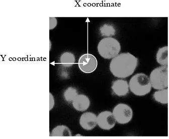
[image:35.612.216.384.212.350.2]image and output center coordinates and radii. An example is shown in Figure 11.
Figure 11. Example of locating X and Y coordinates of a particle’s centroid. The coordinates of centers and radii are calculated by using “imfindcircle” function in Matlab.
Adapted from “Patil, V. R. (2015). A visualization and characterization of microstructures of cohesive powders
(Master’s thesis, Rochester Institute of Technology, Rochester, NY).” Adapted with permission.
A feature from the Leica Application Suite called the Region of Interest analysis
provides the profile of fluorescence intensity as a function of depth (or Z) for a “particle
of interest” demarcated in the region of interest. Patil (2015) found the Z position of the
particle of interest by analyzing the step widths of the layers. Since the distance between
layers was the same, he could find the Z position of a particle by identifying the layer that
contained it.
The Z position of the particle was determined by comparing the radius of the
particle of interest at different depths. In this analysis, the particle ‘starts’ from the frame
when it appears in the XY cross-sectional image and ‘ends’ at the frame where it
X coordinate
24
disappears in the image at a particular depth. This method estimated the Z value for the
particle centroid to be the Z location of the frame where the particle of interest had the
maximum radius. Shown in Figure 12 are cross-sectional images for a particle at two
different depths to illustrate how radius changes at different Z values.
[image:36.612.183.465.199.315.2]
Figure 12. Example of sampling a “particle of interest” at different Z values in two image frames. Radius of the particle varies as the particle cross-section changes from the first frame (depicted in (a)) to the middle frame (shown in (b)). Adapted from “Patil, V. R. (2015). A visualization and characterization of microstructures of cohesive powders
(Master’s thesis, Rochester Institute of Technology, Rochester, NY).” Adapted with permission.
Correspondingly, one can also observe other particles “appearing” or
“disappearing” from each of the views, revealing particles centered at various Z
positions. As the size of a particle increases in the image stack, the number of fluorescing
pixels increases, causing the particle to look bigger and brighter. Beyond the center plane
of the particle, the particle ‘disappears’ or blurs out of the image as the number of
fluorescing pixels decreases. The maximum-radius z-position frame that was previously
identified was next used to locate the X and Y values for the “particle of interest.” To
identify the X and Y coordinates and the radius for the particle of interest, Patil (2015)
used the “imfindcircles.m” function as we mentioned before.
For ease of discussion, Patil’s (2015) method is called the “frame-by-frame
25
method” in the present thesis and the new method developed in this thesis is called the
“3D particle sighting method.” Patil’s method used the algorithm of Hough Transform,
which was conducted in 2D, so that in order to locate the centroid of particles, he had to
run Hough Transform frame by frame. This is not automated and not efficient. In this
thesis, the researcher developed a new automated methodology of 3D convolution to
locate the centers of electro-photographic toner particles. Since this thesis adapted images
from Patil’s research and analyzed the same electro-photographic toner powder system
structure, the “frame-by-frame” particle centroid locations can be used as the ground
truth for comparison with the results generated by the 3D particle sighting method
developed in this thesis.
As discussed in particle centroids detection in colloidal system, the CLSM suffers
from the PSF. In Patil’s research, the Z-axis PSF was ignored because the CLSM he used
at Rochester Institute of Technology had already utilized the PSF correction. When
obtaining a 3D visualization of the sample imaged under the confocal microscope, the
CLSM was equipped with an imaging software suite having deconvolution factors built
into the software for PSF correction. In this thesis, the researcher also ignored the PSF
because the images were coming from Patil’s research.
The researcher had reviewed particle centroids detection techniques in both the
colloidal system and the powder system, including a detailed description of Patil’s
frame-by-frame method the result of which was used as a reference in the present thesis. All
methods had limitations in that they were either not automated or used immersion oil for
26
microstructure analysis. Therefore, there is a need for an automated method to detect the
centroids of dry toner powder particles. In this thesis, the researcher used the 3D
convolution method to detect the centroids of dry toner particles. The three-dimensional
image analysis techniques using 3D convolution are reviewed in the next section.
Three-dimensional Image Analysis: Kernel and Convolution
As discussed in Chapter 2, kernels are a special kind of filter that can be used to
locate the centroids of particles in an image. The result of applying a kernel to an image
is a convolution. The 3D convolution has been successfully utilized in human action
recognition (Xu, Yang & Yu, 2013), shape feature extraction (Suzuki et al., 2006; Pierce,
2011), solid texture analysis (Hopf & Ertl, 1999), and vector distance field (Fournier,
2011). The reason why 3D convolution can be applied in these fields is that 3D
convolution is typically applied to center detection, edge detection, feature extraction,
and noise reduction (Hopf & Ertl, 1999; Kim & Han, 2001; Kim & Casper, 2013; Suzuki
et al., 2006; Xu, Yang, & Yu, 2013). Studies on different applications of both 2D and 3D
convolution are reviewed next.
Cheezum, Walker, and Guilford (2001) added realistic noise to a two-dimensional
image of circles to compare different algorithms for accuracy and precision. They found
that the direct Gaussian fit algorithm, which was using a Gaussian kernel to perform
convolution with the image, was the best algorithm when detecting the centers of circles
in two dimensions in terms of both accuracy and efficiency.
27
image analysis. For example, Suzuki et al. (2006) used 3D convolution for solid texture
detection. They studied shape feature extraction by extending Laws’ (1979) texture
energy approach. In their approach, the Laws’ texture kernels are convolved together to
generate three-dimensional masks. They used the extended 3D Laws’ convolution masks
to analyze 3D solid texture databases. They concluded that the 3D mask may also be
utilized for different 3D solid texture analysis systems, including similarity retrieval,
classification, recognition, and segmentation. This is one example of using 3D
convolution to do center detection and texture extraction.
Another application using 3D convolution is to solve the problem of feature
preserving in mesh filtering, which happens in surface reconstruction of scanned objects.
Fournier (2011) created a new mesh filtering method using 3D convolution to provide an
alternative representation of meshes. An adaptive 3D convolution kernel was applied to
the voxels of the distance transform model. By using error metric evaluations, he showed
that this new design provides high quality filtering results and, at the same time, is better
at preserving geometric features.
As discussed before, Bromley and Hopkinson’s (2002) experiment on centroids
detection of corn flour starch particles was a good example showing the feasibility of
using 2D and 3D convolution to locate the positions of particle centroids. However, they
added immersion oil to their samples, which would affect the 3D structure of the
powders. In this research, we are dealing with images of dry electro-photographic toner
particles adapted from Patil.
28
such as center detection, edge detection, feature extraction, and noise reduction. Different
applications using 3D convolution were utilized in fields including human action
recognition, shape feature extraction, texture analysis, mesh filtering, and so on.
However, 3D convolution has never been used in electro-photographic toner particle
detection. In this thesis, the researcher developed an automated 3D particle detection
method using 3D convolution that makes the particle detection process more efficient
than the existing frame-by-frame method by Patil, by the removing the requirement to
analyze each image frame manually.
Conclusion
The literature on particle centroids detection in both colloidal systems and powder
systems under the CLSM were reviewed. Especially, details of Patil’s frame-by-frame
method of detecting the centroids of electro-photographic toner particles were presented.
The “frame-by-frame” method is not an automated method because it required Hough
Transform to analyze each two-dimensional image frame manually. Literature on the 2D
and 3D convolution techniques showed that convolution can be applied in center
detection, feature extraction, etc., but 3D convolution had never been utilized in a dry
toner powder system to detect the centroids of particles.
There is an opportunity to extend Patil’s (2015) research by using 3D convolution
on the same cross-sectional images from Patil. This thesis seeks to develop an automated
3D particle centroids detection method using 3D convolution. The next chapter presents
29 Chapter 4 Research Objectives
In this thesis, the objective is to develop a new automated and accurate method to
detect the centroids of dry electro-photographic toner particles by using a 3D convolution
algorithm. The images are coming from Patil’s (2015) research on visualizing and
characterizing microstructures of toner particles. Patil’s result of locations of each
particle centroid will be used as the ground truth for comparison with the results
generated by the “3D particle sighting method” developed in this thesis, so that the
accuracy will be assessed. Efficiency will be revealed by comparing the computing time
30 Chapter 5 Methodology
This chapter presents the details of the methodology used to address the research
objectives stated in Chapter 4. First the researcher’s methodology for detecting particle
centers, called the three-dimensional particle sighting approach will be discussed.
Second, the results of Patil’s “frame-by-frame method” will be presented as the ground
truth. Third, the methodology for assessing the accuracy of the three-dimensional particle
sighting approach will be explained. In this research, all image processing algorithms are
31 Three-dimensional Particle Sighting Approach
The flowchart in Figure 13 presents the sequence of steps used in the particle
sighting procedure. It starts with preparing an original stack of images for analysis; this
part is called image enhancement, which includes noise reduction, hole filling, and 3D
matrix generation. The second step is 3D convolution, which consists of applying a 3D
Gaussian kernel to the enhanced 3D image matrix. The third step is to process the 3D
[image:43.612.218.425.309.597.2]convolution matrix to locate the particle centroids.
Figure 13. Flowchart of the three-dimensional particle sighting process, as implemented by the researcher in this thesis.
Image enhancement Start
Locate the centroids of particles Apply 3D convolution
32
Image Enhancement
The first step in the three-dimensional particle sighting procedure is to prepare
original RGB images for analysis using 3D convolution. The image processing
methodology transforms an RGB image into a 3D image matrix as shown in Figure 14. In
this research, all image processing is performed in Matlab, a powerful image oriented
programming language. First, the Matlab “imread” function is used to read the stack of
images into core memory. Second, the “rgb2grey” function is used to transform the RGB
images into gray scale images. Third, the “medfilter” function is used to get rid of noise.
Fourth, the “im2bw” function is used to convert the images into binary images. Fifth, the
“imfill holes” function is used to replace black pixels in the white region with white ones.
[image:44.612.200.448.393.613.2]The last step is to combine all images into a 3D image matrix for convolution.
Figure 14. Flowchart of the image processing procedure. Each step is accompanied by its corresponding Matlab function. The Matlab program for implementing this procedure can be found in Appendix A.
Combine 2D matrices to create a 3D matrix “num2str” function in Matlab
Holes Filled Image “imfill holes” function in Matlab
Binary Image “im2bw” function in Matlab
Noise Reduced Image “medfilter” function in Matlab
Gray Scale Image “rgb2grey” function in Matlab
33
Three-dimensional Convolution
[image:45.612.242.435.171.298.2]The second step in the three-dimensional particle sighting approach is depicted in
Figure 15.
Figure 15. Flowchart for generating a convolution matrix from a 3D image matrix and a 3D Gaussian kernel.
A 3D Gaussian kernel is created by generating algorithms in Matlab (details are
described in Appendix A).
As mentioned in Chapter 2, the 3D Gaussian kernel function is:
F(E,F,G)= 𝐹E∗ 𝐹F∗ 𝐹G= 12Jexp − E:NO
@
2PO@ ∗ 1
2Jexp − F:NQ @
2PQ@ ∗ 1
2Jexp [− (F:NQ)@
2PQ@ ] (3)
F(E,F,G)stands for the 3D Gaussian kernel, which is the result of multiplying FE,
FF and FG. FE, FF and FG are Gaussian function in X, Y, Z directions. For example, in the
X direction, 𝜇E designates its mean value and 𝜎E represents its standard deviation.
Because the maximum value of the Gaussian function is in the center of the graph,
similarly the maximum value of the 3D kernel is likewise located in the center of the
kernel matrix. The 3D image generated is a 256x256x192 matrix, and the kernel is a
40x40x40 matrix. After convolving these 3D matrices, the result is a 295x295x231
matrix.
Read images into Matlab
Generate a 3D Gaussian kernel
34
Locating Particle Centroids
Centroids of individual particles are located at maxima in the 3D convolution
matrix. In order to locate these maxima, the researcher developed a find function in
Matlab. Two versions of the find function were tested. Method A swipes a
three-dimensional assessment matrix through the 3D convolution matrix and compares the
value of the pixel at the center of the assessment matrix to the values of the 6 pixel values
adjacent to it (details of the algorithm are found in Appendix B). Method B swipes the
same three-dimensional assessment matrix through the 3D convolution matrix, but
compares the value of the pixel at the center of the assessment matrix to the values of the
18 pixels surrounding it (details of the algorithm are found in Appendix B). Figure 16
graphically illustrates the difference between the two methods.
[image:46.612.156.478.400.540.2]
Figure 16. Two alternative algorithms for locating particle centroids. (a) depicts the method comparing its central value with 6 pixels surrounding it, while (b) depicts the method comparing its central value with 18 pixels surrounding it.
The Ground Truth
Patil’s frame-by-frame method was reviewed in Chapter 3. This thesis used the
(a) Method A compares the central pixel with six pixels surrounding it.
35
same set of images from his research, so that his results could be used as the ground truth
for the present study. Accuracy is assessed based on the comparison between the ground
truth and the centroids detected by the 3D particle sighting method. Figure 17 shows the
[image:47.612.234.417.200.355.2]centroids detected by Patil’s method.
Figure 17. Ground truth: the centroids of particles detected by Patil with (x, y, z) coordinates. The ground truth is used as a comparison with the results of centroids detection in this research.
Accuracy Assessment
To assess the accuracy of the 3D particle sighting method, the researcher plotted
three-dimensional particle sighting centroids vs the frame-by-frame centroids from Patil’s
research for a sample volume containing 29 particles. The distance between centroids
was then calculated for each particle in the volume. Finally, the researcher assessed the
accuracy of the 3D particle sighting method by comparing these distances to the
diameters of typical toner particles. If the average distance and standard deviation are
small in comparison to the size of the particles being located, then the results can be
36 Chapter 6
Results
This chapter presents the results of applying the “3D particle sighting method” to
detect the centroids of toner particles. Firstly, the results of applying (a) image
enhancement, (b) the 3D convolution process, and (c) the centroids locating process to
the RGB images previously analyzed by Patil are presented. Secondly, the accuracy of
the 3D particle sighting method is assessed by comparing the positions detected using
this method with the “ground truth” positions detected by Patil. Finally, the efficiency of
the 3D particle sighting method is evaluated.
Three-dimensional Particle Sighting Results
This section first presents the results obtained from applying the image
enhancement methodology to Patil’s RGB images. Next, the results obtained by
convolving the 3D image matrix created by the enhancement process with a Gaussian
kernel are presented. Finally, the results of locating the particle centroids in the 3D
37
Results of Image Enhancement
This section discusses the results of experiments using the image processing
methodology. Figure 18 shows the results of applying the final image processing
methodology as developed by the researcher.
[image:49.612.107.545.199.280.2]
Figure 18. Process of image enhancement from an original RGB image (depicted in (a)) to a filled binary image (shown in (e)). In the filled binary image, the white particle has a clear boundary.
Initially, the researcher adopted a simplistic image processing methodology
consisting of only two steps: (a) convert an RGB image into a gray scale image, and (b)
apply a median filter to the gray scale image to reduce the level of noise in the image. In
Figure 18, the original RGB image 18 (a) is transformed into a gray scale image 18 (b)
and, subsequently, filtered to produce the image shown in 18 (c). Unfortunately, when the
researcher convolved the resulting image matrices with a 3D Gaussian kernel, the result
was a collection of maxima (candidate particle centroids) rather than a single maximum.
Investigation showed that the cause of this problem was the varying gray levels of the
pixels in the background and particle areas of the image. The varying gray levels were
confounded with the varying values of the kernel in such a way that local maxima could
be created even when a substantial portion of the kernel overlapped the background area.
This led the researcher to understand the fundamental problem associated with
38
using gray scale images: they do not adequately differentiate background pixels from
pixels in particles. The researcher solved this problem by converting the noise-reduced
gray scale images into binary images. In the resulting binary images, particle region
pixels are converted to ones and background pixels are converted to zeros. Figure 18 (d)
shows the result of this conversion. Notice that the particle pixels are vividly separated
from the background pixels. When the researcher convolved binary images with a 3D
Gaussian kernel, the results were much more encouraging. Most particles showed a single
maximum value in the convolution matrix. Nevertheless, some particles in the binary
images contained black areas inside the particle boundary, and the presence of these areas
resulted in the centroids of such particles being inaccurately located.
To eliminate the problem caused by black voids, the researcher added one
additional step to the image processing methodology. Specifically, the researcher used
the “imfill holes” function in Matlab to fill the holes inside the particle regions. The
resulting image is shown in Figure 18 (e). With this modification, convolving the
resulting 3D matrices with a 3D Gaussian kernel produced clear centroids.
Results from the Three-dimensional Convolution Process
Computing time and accuracy are two factors that need be considered when
choosing a kernel size. Three kernel sizes (40x40x40 pixels, 50x50x50 pixels, and
60x60x60 pixels) were tested using a 50x50x50 sample from the image matrix created by
the enhancement process. The results showed that the location of the centroids detected
39
for the full 256x256x192 image were 30 minutes for a 40x40x40 kernel, 70 minutes for a
50x50x50 kernel, and over 200 minutes for a 60x60x60 kernel. Since the results are the
same and equally accurate, the 3D Gaussian kernel used in this research was a 40x40x40
matrix, the 3D image matrix was 256x256x192, and convolution resulted in a
295x295x231 matrix.
Centroids of Particles
As discussed in Chapter 5, two methods were tested in order to choose the
preferred approach for locating particle centroids. Method A compares the central pixel
in an assessment matrix with the 6 pixels adjacent to it. Method B compares the central
pixel with 18 pixels surrounding it. For some particles, Method A detected multiple
centroids, although the particle itself had only one center. In contrast, Method B typically
detected a single centroid. As a result, the researcher used Method B to detect 29
centroids of particles in one of Patil’s samples, specifically Sample 9. The coordinates of
[image:51.612.107.568.551.704.2]detected particle centroids are shown in Table 1.
Table 1.
Coordinates (in microns) of 29 particle centroids detected by 3D particle sighting approach.
1 2 3 4 5 6 7 8 9 10 11 12 13 14
X 14.74 21.61 12.15 27.35 34.04 40.65 26.94 14.3 22.26 7.09 26.91 9.61 22.22 5.87
Y 39 38.48 32.71 36.39 25.61 23.78 18.35 17.52 12.17 16.48 26.39 30.22 7.09 18.13
Z 4.76 4.76 4.42 7.31 5.61 5.61 5.61 4.34 4.34 4.59 12.24 11.9 13.26 12.92
15 16 17 18 19 20 21 22 23 24 25 26 27 28 29
X 17.96 3.69 10.48 5.52 29.09 12.39 32.74 33.61 31.69 18.3 24.65 8.15 17 18.82 13.7
Y 20.22 31.52 34.13 39 5.17 15.96 17.52 40.91 32.83 34.3 27.69 13.35 31.97 17.17 17.09
40
For visual interpretation, Figure 19 plots the positions of the detected centroids as
[image:52.612.234.414.145.291.2]points inside the sample volume.
Figure 19. Plot of particle centroids detected by the 3D particle sighting method. Each center is shown as a small circle inside the sample volume.
Result of Accuracy Assessment
The accuracy of the 3D particle sighting method was assessed comparing its
results to the results of Patil’s work. Patil (2015) had previously measured the locations
and radii of particles in 9 toner samples using the frame-by-frame method. Appendix C
shows spheres corresponding to the radii and positions measured by Patil in each of the 9
sample volumes. Sample #9, the sample with the largest number of particles, was used to
assess the accuracy of the 3D particle sighting method as compared to the
frame-by-frame method.
To compare the two methods, the researcher retrieved the 2D images associated
with Sample #9. The processing methodology previously described was used to create a
3D image matrix that was convolved with a 3D Gaussian kernel to produce a 3D
41
using Method B as previously discussed. These locations were compared to the locations
of the centroids identified using the frame-by-frame method. The results revealed that the
average delta distance between centroids was 1.02um with a standard deviation of
0.93um.
Figure 20 is a three-dimensional plot showing the proximity of the calculated
centroid locations. Small triangles represent centroids detected using the frame-by-frame
method; small circles represent centroids detected by the 3D particle sighting approach.
[image:53.612.135.511.337.547.2]Paired results for individual particles are encompassed by black ellipses.
Figure 20. Agreement between 3D particle sighting results and frame-by-frame results. Small triangles depict the centroids located by Patil, ground truth for the researcher’s comparison. Small circles depict centroids located by the 3D particle sighting method. Corresponding centroid pairs are circled in black ellipses.
Although the overall results of using the 3D particle sighting method are strongly
positive, there is still room for improvement. As shown in Figure 21, the majority of
: 3D particle sighting center : Frame-by-frame center