Balancing wheeled robot

University of Southern Queensland

Faculty of Engineering and Surveying

Balancing Wheeled Robot

A dissertation submitted by

Ho, Khoon Chye Randal

in fulfillment of the requirements of

Courses ENG4111 and 4112 Research Project

towards the degree of

Bachelor of Engineering (Electrical and Electronics)

Certification

I certify that the ideas, designs and experimental work, results, analyses and conclusions set out in this dissertation are entirely my own effort, except where otherwise indicated and acknowledged.

I further certify that the work is original and has not been previously submitted for assessment in any other course or institution, except where specifically stated.

Ho, Khoon Chye Randal Student Number: 0050027382

__________________________________

Signature

Faculty of Engineering and Surveying

Limitations of Use

The Council of the University of Southern Queensland, its Faculty of Engineering and Surveying, and the staff of the University of Southern Queensland, do not accept any responsibility for the truth, accuracy or completeness of material contained within or associated with this dissertation.

Persons using all or any part of this material do so at their own risk, and not at the risk of the Council of the University of Southern Queensland, its Faculty of Engineering and Surveying or the staff of the University of Southern Queensland.

This dissertation reports an educational exercise and has no purpose or validity beyond this exercise. The sole purpose of the course pair entitled “Research Project” is to contribute to the overall education within the student’s chosen degree program. This document, the associated hardware, software, drawings, and other material set out in the associated appendices should not be used for any other purpose: if they are so used, it is entirely at the risk of the user.

Prof G Baker

Dean

Faculty of Engineering and Surveying

Acknowledgements

I would like to express sincere thanks to my USQ project supervisor Mr. Mark

Phythian local supervisor for their guidance and support throughout the duration of the balancing wheeled robot project. I have learned a lot under their guidance, be it

practically or theoretically.

In addition to that, I would also like to thank lab supervisor Mr. Voon who has help me to arrange the suitable lab hours to use during the course of the project. He is indeed a nice person as no matter how busy he would offer some time to give some invaluable advice on certain issues.

Other than that I am also grateful to my friends who have help and guide me in searching for important notes and books.

Abstract

Inverted pendulum has long been the interest of control engineers. The system is unique in such a way that defies the logic of human brain. Moreover, the system inherited the non-linearity attributes, which is part of every systems on earth.

The concept of two wheeled balancing robot is based on the inverted pendulum theory. A suitable control system is needed to control the system so that it is balanced and stable. The main purpose of this project is to use a good control strategy to keep the body of the robot upright.

This dissertation applies the idea of non-linear control strategy and analyses its effectiveness. The non-linear control strategy requires a good understanding of the inverted pendulum system. The knowledge is then implemented in programming to program the microcontroller. This is particularly important in low-level assembly language, which is used in this project.

Two types of semiconductor sensors to provide tilt information to the robot to balance are applied. The sensors used are gyroscopes and accelerometer. The performance of the sensors is then evaluated based on stability.

The following are the variables being used in modeling the balancing robot. x Linear displacement

x& Linear velocity

x&

& Linear acceleration

θrc Rotation angle of robot chassis

θ

&

_rc Angular velocity of the robot chassis

θ

&

&

_rc Angular acceleration of robot chassis

θ

&

_wh Angular velocity of the wheel

θ

&

&

_wh Angular acceleration of the wheel Cl Applied torque from motor to left wheel Cr Applied torque from motor to right wheel Pl, Pr Reaction forces between the wheel and chassis Hl,Hr

Hfr,Hlr Friction forces between the wheels and the ground g Gravitational acceleration, 9.81m

s

−2

J

rc Moment of inertia of robot chassis

J

wh Moment of inertia of wheelw

M

wh Mass of the robot wheels

M

rc Mass of robot chassis

Page

Certification

i

Limitation of Use

ii

Acknowledgements

iii

Abstract

iv

Nomenclature

v

Chapter 1: Literature review

1.0

Balancing Robots

1

1.1 Control System

2-3

1.2

Data Acquisition

4

1.3

Kalman Filter

4

Chapter 2: Introduction

2.0 Balancing Wheeled Robot Concept

5

2.1 Balancing Process

5-6

2.2 System Modeling

2.2.1 Wheel Modeling

7-9

2.2.2 Chassis Modeling

10-13

3.0 Motor Selection

15

3.1 Speed Calculation

15-16

3.2 Motor Capacity

3.2.1 Speed Measurement

17

3.2.2 Results

18

3.4

Robot Chassis Design

3.4.1 Robot Weight

19

3.4.2 Materials

19

3.4.3 Robot Response

19

3.4.4 Gears Selection

20

3.4.5 Motor Mounting

20

3.4.6 Aluminum Rod Fabrication

21

3.4.7 Rigidity

21

3.4.8 Robot Chassis Construction

22

Chapter 4: Sensors

4.1

ADXRS 300 Gyro

23

4.2

Coriolis Acceleration

24

4.3

Coriolis Acceleration on Gyro

24-25

4.4

Measuring Coriolis Acceleration

25-26

4.5

Advantages

26

4.6

Axis Selection

27

4.7

Mounting

28

4.8

ADXRS Gyro as Tilt Meter

29

4.11 Calibration

4.11.1 Power Supply Decoupling

30

4.11.2 Capacitors

31

4.11.3 Calculation

31

4.11.4 Software Approach

32-33

4.12

Overall Balancing Program

4.12.1 Programming Approach

34

Chapter 5: Stability Analysis

5.1 Differential Drive Motor Control (While Standstill) 36

5.2

Sensor Fusion

36-38

5.3

Averaging

39

5.4

Differential Drive Motor Control (While Traveling) 39

Chapter 6: Motor Control

6.1

Pulse Width Modulation

40

6.2

H-bridge design

6.2.1 Introduction

41-43

6.3

Design Consideration

43-44

6.4

Totem-pole Circuit

45-46

6.5

Unwanted Situation

46

6.6

Experiment

47

6.7.2 Current Surge

48

6.7.3 Noise Isolation

48

Chapter 7: Microcontroller

7.1

Reasons

49-50

7.2

Memory

51

7.3

Time Consideration

7.3.1 Oscillators

52

7.4

Software

53

7.5

Arithmatic Operation

54-55

7.5.1 Trade-off

56

Chapter 8: PCB Design Consideration

57

Chapter 9: Discussion & Conclusion

9.1

Result

9.1.1 Gyro Mounting

58

9.1.2 Accelerometer

58

9.2

Reasons

58-59

9.3

Incomplete tasks

9.3.1 Gyro-Accelerometer Combo

59

9.4

Conclusion

References

Page

Figure 1: Difference between linear and non-linear response

3

Figure 2: Inverted and non-inverted pendulum

5

Figure 3: Equilibrium or Balanced State

6

Figure 4:

Tilted or Unbalanced State

6

Figure 5: Free body diagram of the wheel

7

Figure 6: Inverted Pendulum Free body diagram

9

Figure 7: Balancing robot control system

13

Figure 8: Speed measurement using tachometer/stroboscope

17

Figure 9: Aluminum Gear mounting

20

Figure 10: Motor Mounting

20

Figure 11: Aluminum rod fabrication and mounting

21

Figure 12: Nut tightening

21

Figure 13: Robot Chassis

22

Figure 14: Cut away view of robot base mounting

22

Figure 15: ADXRS 300 Gyro

23

Figure 16: Coriolis acceleration on earth

24

Figure 19: Complete inner gyro structure

26

Figure 20: ADXRS 300 Gyro Axes

27

Figure 21: Gyro mounting

28

Figure 22: Gyro characteristic curve

29

Figure 23: PCB power supply coupling

30

Figure 24: Duty cycle decoding scheme

32

Figure 25: Pulse Width Modulation waveform

40

Figure 26: Motor clockwise turn

41

Figure 27: CEMF current flow

42

Figure 28: Motor counter clockwise turn

43

Figure 29: Totem-pole and P-channel Mosfet

45

Figure 30: N-channel MOSFET motor driver

47

Figure 31: Pulse train waveform

47

Figure 32: Clean pulse train waveform

48

Figure 33: Noise corrupted pulse train waveform

48

Figure 34: Microcontroller schematic diagram

49

Figure 35: Microcontroller memory

51

List of Tables

Page

Table 1: Motor O Speed Characteristics

18

Table 2: Motor X Speed Characteristics

18

Table 3: Analog to digital conversion

34

Table 4: H-bridge circuit components operation

44

Table 5: MOSFET’s operation

45

Chapter 1: Literature Review

This section provides an insight and literature review to the current technology available to construct a two-wheel self balancing robot. It also highlights various methods used by researches on this topic.

1.0 Balancing robots

The concept of balancing robot is based on the inverted pendulum model. This model has been widely used by researches around the world in controlling a system not only in designing wheeled robot but other types of robot as well such as legged robots.

Researches at the Industrial Electronics Laboratory at the Swiss Federal Institute of Technology have built a prototype two wheel robot in which the control is based on a Digital Signal Processor. A linear state space controller using information from a gyroscope and motor encoder sensors is being implemented to make this system stabilise. (Grasser et al.2002).

Another two wheeled robot called ‘SEGWAY HT’ is available commercially (Dean Kamen ,2001) . It is invented by Dean Kamen who has design more than 150 systems which includes climate control systems and helicopter design. An extra feature this robot has is that it is able to balance while a user is standing on top of and navigate the terrain with it. However, this uses five gyroscopes and a few other tilt sensors to keep it balanced.

Steven Hassenplug used a more innovative approach to construct a balancing robot (Steve Hassenplug, 2002). The chassis of the body is constructed by using the LEGO Mindstorms robotics kit. The balancing method of controlling the system is unique with two Electro-Optical Proximity Detector sensors is used to provide the tilt angle

information for the controller. This omits the conventional use of gyroscope that has been used by previous robot researchers.

1.1 Control System

Over the years there are only two types of control being used by researchers in

controlling a system. The types of control is categorised as linear and non-linear control.

In some instances, the linear control is sufficient to control a system. One of the most widely used is the Proportional Derivative Integral controller or better known as the PID controller (Rick Bickle, 2003). The others are linear quadratic controller (LQR), fuzzy logic controller, pole placement controller etc. It is generally accepted that linear control is more popular than non-linear control.

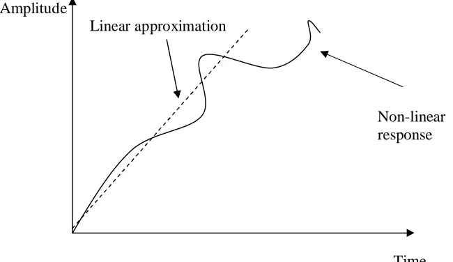
There are two reasons for this. In all cases, the modeling of a system requires a lot of parameters to be considered and applied. Therefore, the system is complex. However, some of the parameters values needed to model the system are small. That is why most researchers would prefer to model their applications in a linear approximation, which is simpler and in some instances effective.

However, in most cases the linear control theory is not suitable for real life

Figure below shows how a non-linear response can be approximated to a linear response.

Amplitude

Linear approximation

Non-linear response

[image:17.612.175.500.160.348.2]

Time Figure 1: Difference between linear and non-linear response

1.2 Data Acquisition

In a paper ‘Attitude Estimation Using Low Cost Accelerometer and gyroscope’ presented by Young Soo Suh, it shows the two different sensors which is the accelerometer and gyroscope that exhibits poor results when use separately to

determine the attitude which is referred as the pitch angle or roll angle. The factor that contributes to the deviation of the desired result of the gyroscope is due to the drift term. Since the drift increases with time error in output data will also increase.

One of the disadvantages of using accelerometer individually is that the device is sensitive to vibration since vibration contains lot of acceleration components. One solution that Young suggested is that a low pass filter is required to limit the high frequency.

However, the gyroscope can combine with accelerometer to determine the pitch or roll angle with much better result with the use of Kalman filter.

1.3 Kalman Filter

Chapter 2: Introduction

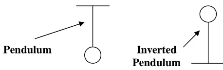
2.0 Balancing Wheeled Robot Concept

Imagine a 2D diagram of an inverted pendulum on the wheel cart. If say, the pendulum falls to the left, the cart should move to the left to try and keep it upwards. This is the same explanation if the pendulum falls to the other side.

[image:19.612.174.403.251.323.2]

Pendulum Inverted Pendulum

Figure 2: Inverted and non-inverted pendulum

2.1 Balancing Process

The figures below show the various position of the robot could be in.

Vertical axis

Figure 3: Equilibrium or Balanced State

Tilted Angle Robot Axis

2.2 System modeling

One of the very first steps for a control system engineer to able to control a system successfully is to understand the system first. An engineer can understand the system better through modeling the system in a free body diagram. In this balancing wheeled robot the modeling is divided into two parts. The first is the wheel model and the second is the chassis model.

After modeling the parameters are combined accordingly in the form of equation. With that the model can be represented by a set of equations in a state space form and controlled using control system theory.

2.2.1 Wheel modeling

Right wheel Left wheel

Pr _θ

wh Pr θwh

Hr Hr

Hfr Hfr

x, x& x&& x, x& &x&

Figure 5: Free body diagram of the wheel

Using the Newton’s law of motion, sum of the forces on the x-direction,

ΣFx = Ma

Cr Mwh

Summing up the moment around the centre of the wheel,

ΣM = Jα

Cr- Hfr*r = Jwh

θ

&

&

wh (11)

Rearranging equation (11),

Hfr = r -wh wh r

J

C

θ

&

&

₍₁₅₎

For the right wheel substitute equation (11) into (10),

Mwh&x& =

r

-wh wh r

J

C

θ

&

&

_{-Hr (16)}

For the left wheel,

Mwh&x& =

r

-wh wh l

J

C

θ

&

&

_{-Hl (17)}

Because the linear motion is acting on the centre of the wheel, angular motion can be transformed into linear motion by simple transformation.

θ

&

&

_whr =x&&,

θ

&

&

wh= _r

x&

&

(18)

θ

&

_whr = x&,

θ

&

wh= _r

x&

(19)

For the right wheel,

Mwh&x&=

r

C

r_-

r

J

wh

For the left wheel,

Mwh&x& =

r

C

l_-

r

J

wh

2 x&&- Hl (21)

Summing up equation (20) and (21),

2(Mwh+

r

J

wh

2 )x&&=

r

C

r₊

r

C

l_{- (Hl + Hr) (22)}

2.2.2 Chassis Modeling

θ

wh

x&

& (Cl + Cr)

J

θ

&

2

rc

Mrcg I

θ

&

&

rc

Hl+Hr

Pl+Pr

Figure 6: Inverted Pendulum Free body diagram

Sum of forces perpendicular to the chassis or pendulum

ΣFperpendicular = Mrc&x&cosθrc

(Pl+Pr)sinθrc + (Hl+Hr)cosθrc - Mrcl

θ

&

&

rc- Mrcg sinθrc = Mrcx&& cosθrc (23)

(Hl+Hr) + Mrcl

θ

&

2

rcsinθrc - Mrcl

θ

&

&

rccosθrc = Mrcx&& (24)

Sum of moments around the centre mass of the pendulum

∑

M = Jα , where α =

θ

&

&

rc

-(Pl+Pr)l sinθrc - (Hl+Hr)l cosθrc- (Cl+Cr) = Jrc

θ

&

&

rc (25)

Rearranging equation 25,

-(Pl+Pr)l sinθrc - (Hl+Hr)l cosθrc = Jrc

θ

&

&

rc+ (Cl+Cr) (27)

Multiplying equation (23) by – ell,

[-(Pl+Pr)sinθrc - (Hl+Hr)cosθrc]l+ Mrcgl sinθrc + Mrc

l

2

θ

&

&

rc= -Mrcl &x& cosθrc (28)

Substitute equation (27) into equation (28) to eliminate (Pl+Pr) and (Hl+Hr) term and rearranging the same terms,

Jrc

θ

&

&

rc+ (Cl+Cr) + Mrcgl sinθrc+ Mrc

l

2

θ

&

&

_rc = -Mrcl x&&cosθrc (29) To eliminate (Hl+Hr) term for the second equation, equation (24) is inserted into Equation (22) and rearranging the same terms,

(2Mwh+

r

J

wh

2

2

_{+ M}

rc)&x&=

r

C

r₊

r

C

l_{+ M}

rcl

θ

&

2

rcsinθrc - Mrcl

θ

&

&

rccosθrc (30)

Equation (29) and (30) are non-linear equations, and to get linear equations, some linearising or assumption are taken. Let θrc= π + δ, where δ is the small angle from the vertical upward direction. Therefore, cosθrc = -1, sinθrc = - δ and

t

d

rc

2 2

The linearised equation representing the whole system is, Jrc

δ

&

&

rc+ (Cl+Cr) - Mrcgl δ + Mrc

l

2

δ

&

&

_rc = Mrcl x&& (31)

(2Mwh+

r

J

wh

2

2

_{+ Mrc)&x&=}

r

C

r₊

r

C

l_{+ Mrcl}

δ

&

&

_rc (32)

Rearranging the state space representation,

δ

&

&

_rc=

(

)

l

M

J

C

C

l

M

J

M

l

M

J

M

rc rc r l rc rc rc rc rc

rcgl l _x

2 2 2 + + − + +

+ δ && (33)

        + + + +         + + =

r

J

M

M

C

C

r

J

M

M

M

wh rc wh r l rc wh rc wh rc r l x 2 2 2 2 2 2

δ

&

&

&

& (34)

The state space equation is obtained as below after substituting equation (33) into (32) and equation (34) into (31) in the form of:

                                  − − + − + − +                                                         + − + − =              

C

C

M

M

l

M

J

M

l

M

J

M

l

M

l

M

J

l

M

l

M

J

l

M

l

M

l r rc rc rc rc rc rc rc rc rc rc rc rc rc rc rc rc r l r l l r l r x x g g x x 1 1 0 0 1 1 0 0 0 0 0 1 0 0 0 0 0 0 0 0 1 0 2 2 2 2 2 2 2 2 2 2 2 2 ϕ ϕ δ δ ϕ ϕ δ δ & & & & & & & & (35)

where ϕ=

M

r

J

M

rc

wh wh+ 2 +

2 2

and output of y = Cζ

                    = δ δ & & x x y 0 1 0 0 0 0 0 1 (36)

Applying the feedback equation:

u = r –

            4 3 2 1 ] [ x x x x h g f e (37) Whereby x1, x2, x3 and x4 are the states of the state space equation

The feedback equation is the equation that is about to be inserted into the main system, with coefficients e,f,g, and h are the arbitrary chosen values to be experimented (by trial and error) in order to get the robot to balance properly.

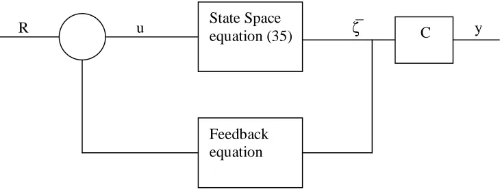
Finally the overall balancing robot control system is shown in the figure below.

[image:27.612.150.515.365.505.2]

R u ζ y

Figure 7: Balancing robot control system

The term or variable u represents the driving speed of the motor to lift the robot chassis upright. In order to drive the robot chassis upright the motor need to have the required minimum speed to do the task.

The non-linear state space equation is difficult to derive as there are many variables that State Space

equation (35)

Feedback equation

2.3 Approach

The balancing robot can be controlled using the state space equation with high level language programming such as C. However, after gaining much understanding of the robot system it is logically possible that the balancing robot can be controlled by using the assembly language programming, even though it is quite simplistic as compared to the state space equation previously derived in the modeling section.

The following strategy is applied in the control of balancing robot.

a)Data acquisition time

The time the microcontroller takes to collect and execute the data obtained. Theoretically if the microcontroller can acquire data and applying control strategy faster than the response of the robot chassis tilts the robot will appear to be balanced and more stable.

b) The non-linearity control

Applying a control strategy limits the overshoot. For instance, there is no accurate prediction that the motor would not output more speed when in fact the speed required to control (programmed) is lesser. That is why to be on the safe side a few lines of control to limit that possible non-linearity behavior.

c) Proportional band control

Chapter 3: Hardware

3.0 Motor Selection

There are basically two types of motor that are in consideration initially. There are a few reasons why the car wiper motor, which is one of the permanent magnet DC motor, is chosen over stepper motor.

The first is that the stepper motor does not turn on the shaft fast enough. That is the speed of response is slow. This could be detrimental to the balancing robot as the speed that the robot tilts is quite fast and need a motor that could match or have faster

response than the robot chassis to lift the chassis to the upright position.

Secondly, the rating speed (in r.p.m) of the stepper motor is not as high as the

permanent magnet DC motor. This aspect is also essential in the balancing robot project as heavier robot needs more motor speed from the motor to lift the chassis balanced state.

3.1 Speed Calculation

This section focuses on the how to calculate the required speed of the motor to lift the chassis of the balancing robot upright. The rated speed of the motor has to be

sufficiently high in order to balance the weight of the robot. If the weight of the robot is more than the motor can handle the robot will not be able to standstill.

Acceleration needed = 5ms-2

Force to accelerate the 2kg is F=ma, F= 2*5ms-1

= 10N (5 N per wheel) Wheel radius = 0.045m

Power required from motor would be P = v * F = 2 *10

= 20W , that is two 20W motors

Assuming the motors will on average operate at ½ their rated voltage, this leads to a factor of 4 reductions in the power output of the motor (from its rated power).

P= V2/R = (1/2V)2/R = 1/4V2/R

So that is 20W (needed) * 4 = 80W motors.

Given some tolerance of 5% of the required power of the motor; therefore a motor power rating of about 84W is required.

3.2 Motor capacity

After finalising the required speed of a motor needed the next step would be confirming the motor capacity of a motor practically. The information can be obtained by reading

the angular rate or speed and power from the motor’s datasheet. Since the car wiper

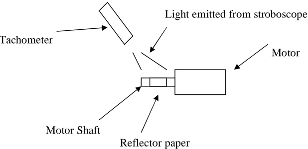
motors that obtained is from the spare parts shop another method is needed to get the information. This can be by using a stroboscope/tachometer to measure the angular rate.

3.2.1 Speed measurement

Light emitted from stroboscope Tachometer

Motor

Motor Shaft

[image:31.612.136.445.306.456.2]

Reflector paper

Figure 8: Speed measurement using tachometer/stroboscope

3.2.2 Results

Determining the characteristics of the wiper motor: Motor O (Side wire)

Voltage, V Current , A Angular speed, rpm

12V 1.3A 3100 rpm

10V 1.26A 2500 rpm

8V 1.05A 1900 rpm

Motor O (Centre wire)

Voltage, V Current , A Angular speed, rpm

12V 0.7A 2100 rpm

10V 0.68A 1780 rpm

8V 0.6A 1360 rpm

Table 1 : Motor O speed characteristics

Motor X (Side wire)

Voltage, V Current , A Angular speed, rpm

12V 1.8A 3000 rpm

10V 1.7A 2300 rpm

8V 1.6A 1770 rpm

Motor X (Center wire)

Voltage, V Current , A Angular speed, rpm

12V 1.22A 2085 rpm

10V 1.2A 1700 rpm

8V 1.12A 1300 rpm

Table 2 : Motor X speed characteristics

3.4 Robot Chassis Design

3.4.1 Robot Weight

It is important to consider the overall weight of the robot that one is about to build. This would seriously affect the wheel base design of the robot. The base and the wheel might bend outwards if the overall weight of components is too high for the wheel base to handle.

The drop down list of the total weight contributed:

Quantity kg/quantity Total weight (kg) Sealed lead acid battery 2 1 2

Aluminum - 0.5 0.5 Wiper motors 2 0.5 2

Printed Circuit Boards 4 0.02 0.08 Total = 4.58kg From the total weight anticipated the robot requires a strong wheel base.

3.4.2 Materials

Since the aluminum is strong, light and affordable it is preferably chosen as the material to build the robot base and chassis.

3.4.3 Robot Response

3.4.4 Gears Selection

The tooth gear pulley is chosen ahead of the sprocket type. This is because the tooth gear pulley is more durable and the quietest choice. The tooth belt pulley consists of two aluminum gears and a suitable length of belt. This method is easy to use and do not require special skill to mount on the robot.

[image:34.612.256.411.211.316.2]

Figure 9: Aluminum Gear mounting

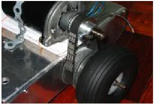
3.4.5 Motor Mounting

Since the wiper motor is quite heavy and a tooth gear pulley is required, it is best that the motor is mounted on top of the robot wheel base. In addition to that ball bearing is embedded into the aluminum side plate in an axis parallel to the motor shaft. This is to reduce the amount of friction imposed on the shaft and this enable the shaft to turn smoothly.

[image:34.612.255.410.517.620.2]

3.4.6 Aluminum rod fabrication

This step is taken to ensure the portability of the robot. The top and middle rods can be disconnected anytime the user wants.

[image:35.612.142.510.172.278.2]

Figure 11: Aluminum rod fabrication and mounting

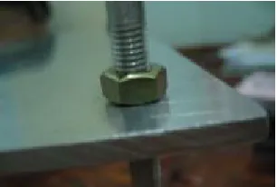
3.4.7 Rigidity

This type of tightening is to ensure that the robot do not wobble while balancing.

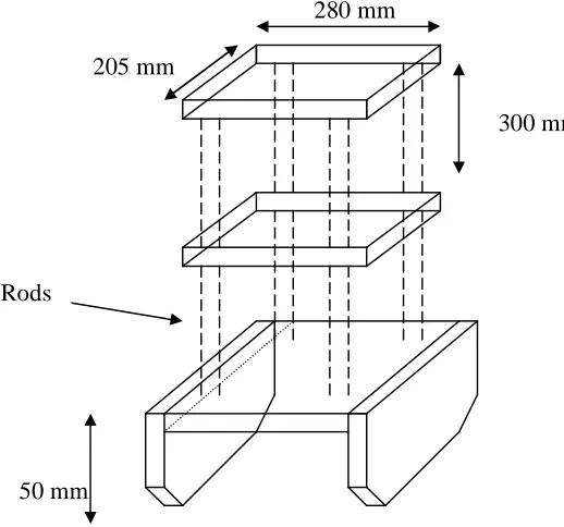
[image:35.612.258.411.433.536.2]

3.4.8 Robot Chassis construction

The chassis of the robot will be constructed of the following designs:

280 mm 205 mm

300 mm

Rods

50 mm

[image:36.612.177.436.148.390.2]

The mounting of the motor to the wheel

Figure 13: Robot Chassis DC wiper Motor

Gear teeth Shaft

Wheel Bearings in each plate

Gear teeth

[image:36.612.138.481.455.623.2]

Chapter 4: Sensors

The feedback block of the balancing robot control system consists of sensors that provide information for the robot to move accordingly. There are two types of sensor used in this project, which are the gyro and the accelerometer.

4.1 ADXRS 300 Gyro

A person might be curious on how the ADXRS gyro measure data to provide important information to the balancing wheeled robot. It is a general statement that gyro

[image:37.612.242.425.359.468.2]

measures angular rate of turn data. ADXRS gyro obtains this data by measuring the coriolis acceleration.

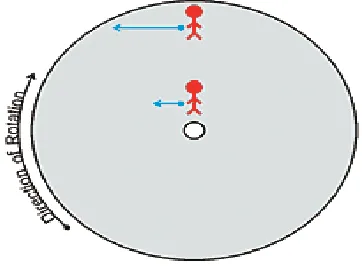
4.2 Coriolis acceleration

[image:38.612.242.423.241.374.2]

Imagine a person standing on a rotating platform near to the center trying to maintain his position to the ground by walking against the rotation at a given speed. Whereas if a person were to maintain his position at the outer rotating platform (away from the center) he has to increase his movement speed. The increase in speed is termed coriollis acceleration (John Green et al, March 2003).

Figure 16: Coriolis acceleration on earth (Source: John Green et al, March 2003)

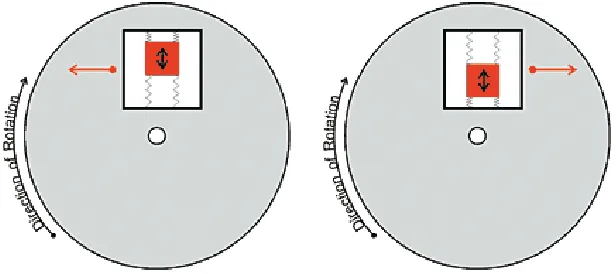
4.3 Coriolis acceleration on gyro

Figure 17: Gyro rotation behaviour (Source: John Green et al, March 2003)

4.4 Measuring coriolis acceleration

[image:39.612.180.488.129.266.2]

The figure below shows the cut off structure of the ADXRS 300 gyro. The structure frame containing the mass is tethered to the substrate perpendicular to the resonating motion (John Green et al, March 2003). The ADXRS primarily utilises the coriolis sense fingers to ‘read’ the amount of force applied by the mass to it, which in turn ‘translates’ the force into the voltage reading.

Figure below is the complete structure of the ADXRS gyro placed on the moving plate.

Figure 19: Complete inner gyro structure (Source: John Green et al, March 2003)

4.5 Advantages

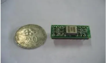
There are quite a number of reasons why this gyro sensor is chosen over the other sensors such as tilt meters and gyro for helicopters. The reasons are as follows:

i) Small in size

There is no need to worry about space. Since the gyro is so small that is only about the size of a coin the user can place the gyro on a small empty space on the robot.

ii) Samples available for free (from www.analogdevices.com)

This is great for any researchers that are keen on researching but short of funding. Analog devices provide this golden opportunity for anyone to try hands-on.

iii) Has internal conditioning on-chip

iv)Readily available for interfacing with microcontroller chip

There is no need to include extra circuits to interface the ADXRS 300 gyro with microcontroller chip as the signals are compatible with each other.

4.6 Axis selection

[image:41.612.139.421.286.409.2]

There are a few axes that can be used. There are named Yaw Axis, Roll Axis and Pitch Axis as shown in figure (A) below. In the balancing robot application only one axis is used. This can be the roll axis in figure (B).

4.7 Mounting

[image:42.612.207.511.232.520.2]

Due to the fact that measurement of coriolis acceleration is most sensitive when mounted parallel to the ground surfaced the gyro has to be mounted on like the one in the figure(B) above onto the robot. The mounting can be as shown below:

Figure 21: Gyro mounting

Gyro

Gyro axis

4.8 ADXRS Gyro as tilt meter

Based on the graph given below the range of values from 2.5 to 4.75 volts can be assigned for clockwise direction tilt and from 2.5 to 0.25 volts the values can be allocated for anti-clockwise direction. For instance, when the microcontroller receive an input on 4.0 volts the chassis will tilt clockwise direction and motor will turn anticlockwise to lift the chassis back up and vice versa.

Figure 22: Gyro characteristic curve

4.9 Measurement Range

The ideal measurement range of the graph above does not apply to the practical

measurement range. Initially, the measurement range of the gyro is only within 2.3 to 3 volts. Therefore, the method of extending the range is by adding a resistor between the pins CMID and SUMJ of the gyro. This can be found in the data sheet as attached in appendix C4. As found out the measurement range is only from 1.8 volts to 4.9 volts. As a result some adjustment has to be made to enable the microcontroller to measure the voltage values.

0.25v

4.75v

2.5v Tilt

4.10 ADXL Accelerometer

The purpose of this accelerometer is to be examined whether it can be used as an alternative to find the tilt angle. The second purpose of accelerometer can be considered to use with the gyro chip to stabilize the angular reading drift. This is because it may have an important property, which is the duty cycle to hold the data for a specified period of time before the next sampling edge to calculate and replace the old value.

4.11 Calibration

With reference to the data sheet attached at the appendix C3.There are a few electronic components values that needed to be determined before mounting on the printed circuit board designed as attached at the appendix B1.

The primary function of the Rset resistor is to set the PWM period of the accelerometer output, T2. The equation is given in the equation below:

T2 = Rset/125MOhm

4.11.1 Power supply decoupling

Vdd

Rextra

Cdc

[image:44.612.144.424.462.619.2]

Rextra = 100 Ohm or less. Cdc = 0.1uF

Figure 23: PCB power supply coupling Vdd

4.11.2 Capacitors

The capacitors Cx and Cy act as the filtering system to reduce the external noise that might affect the overall performance of the accelerometer.

Choosing the low pass filter bandwidth to be 100Hz Using the equation: F-3dB=1/(2π (32KOhm)*C(x,y)) Therefore, the capacitance value would be = 0.05uF

4.11.3 Calculation

The calibration of ADXL 213 is done by utilizing the earth’s gravity as a reference input. The X and Y axes are properly aligned horizontal to the earth such that both axes experience 0g. A microcontroller is told to read the duty cycle output T1 and period T2 from each of the axes.

The accuracy can be improved by average the readings of T1 and T2. These values are used as the fixed values to be used in calculating the acceleration after calibration mode.

Zcal = (T1max – T1min)/2

The bit scale factor is to be found next. This is to determine the resolution (in bits) of the acceleration calculation as shown below:

4.11.4 Software Approach

T2actual is the measurement of T2. This formula offsets the 0g value for changes in T2 due to drift. The steps below are actually the method that is used to sample the edges of the output pulse of the accelerometer output.

T2

T1

Xout

[image:46.612.133.432.201.296.2]

Ta Tb Tc

The flow chart below illustrates the sampling of the output edges

As can be seen above only the output pulse at X pin is being sampled. This is because one axis is sufficient in this application. After sampling the time values the

Acceleration and tilt value of axis can be found by using the formula below:

Acceleration = K*(T1-Zactual)/T2actual Zactual = (Zcal * T2actual)/T2cal

Full program listing is attached at appendix D Timer is started

at Ta

Time at point Tb is recorded

Time is for T1 is recorded. T1= Tb-Ta

Time at point Tc is recorded

Time for T2 is recorded T2=Te-Ta

Is samples = 8?

4.12 Overall Balancing Program

4.12.1 Programming Approach

The ADXRS 300 Gyro output is in the form of analog values. Therefore, the Analog to Digital Converter (ADC) Module of the microcontroller is being utilised.

Since the resultant registers storage is of 10 bits wide and the maximum voltage used is 5V therefore the assigned analog voltage to digital form is as shown in table 3.

One bit value is : (2^10)/5 = 1023/5 = 204.6 or equal to 205

Analog (v) Multiplier Digital

1 205 205

1.5 205 308

2 205 410

2.5 205 513

[image:48.612.129.541.303.395.2]

3 205 615

Table 3: Analog to digital conversion

The resultant value is being stored in ADRESH and ADRESL registers.

After that the computer program will calculate the reading error from the reference, which is 3V. Then the direction to control will be determined. The program will appropriately choose the correct subroutine, based on error reading calculated to send the appropriate amount of PWM signal to control the motor. In the way it is

Chapter 5: Stability Analysis

There are some points need to be taken into consideration. There are a few things that could be done in order to properly balance the robot.

5.1 Differential Drive Motor Control (While Standstill)

The method being used here is to manually calibrate the speed of the two differential drive motors such that the shaft not only turns in one direction but with the same speed as well.

The calibration of the two wiper motors are done prior to mount the gyro and accelerometer onto the robot chassis. This is one important step before balancing the robot.

The robot will be quite impossible to balance and might wobble around.

5.2 Sensor Fusion

Both the gyro and accelerometer can be used to measure tilt data. However, only the gyro is used to measure the tilt while the accelerometer can be used as a ‘stabiliser’ to provide stability. There are three important properties that can be utilised from the accelerometer.

The accelerometer provides a true measure of tilt. For example, the accelerometer will output a digital pulse when the device is in steady state condition. Similarly,

accelerometer will change its output accordingly when the device rotates. In other words, the accelerometer will only change its output when the device changes direction.

Unlike the accelerometer the gyro is sensitive to drift, which the value of the output changes with respect to time. For instance, when the gyro rotate to a position, the gyro will give a reading, however, the reading will quickly return to steady state value as there is no angular turn.

No

Yes

T(ms) delay Accelerometer duty cycle sensor output

Gyro output analog voltage

Include accelerometer sensor to compare

Microcontroller output signal to h-bridge

H-bridge output PWM signal to motor to balance the robot

5.3 Averaging

Since the gyro outputs data at a high rate the sensor data is quite unstable. In other words, the reading is not linear and it oscillates. That is why the reading needs to be averaged.

This is one method of reducing the non-linearities. For example let the original data output at a rate of 400Hz and if the data is averaged for eight samples. Therefore the output rate would be 400Hz/8 = 50Hz.

5.4 Differential drive motor control (While traveling)

There could still be deviation of the actual trajectory when the robot is traveling, even though initial calibration as in section 5.1. This is analogous to a situation whereby when a person is driving a car with the steering wheel set such that the car moves in a straight direction. The person just sits there without holding the steering wheel while the car is in motion. After some time, the steering will move and the car moves side ways.

Chapter 6: Motor Control

6.1 Pulse Width Modulation

[image:54.612.150.485.265.388.2]

PWM output is basically a series of pulses with varying size in pulse width. This PWM signal is output from the h-bridge circuit to control the wiper motor. The difference in pulse length shows the different output of h-bridge circuit controlling the output speed of the motor.

Figure 25: Pulse Width Modulation waveform

Figure above shows the varying pulse length of the pulse width modulation (PWM) scheme. Let’s say that the PWM frequency is about 50 Hertz, with a period cycle of 20ms. Therefore assuming that the T1 and T2 length values are 15ms and 5ms respectively, the duty cycle can be calculated as below:

Duty cycle = T1/(T1+T2) * 100% = 15/20 * 100% = 75%

Therefore if the maximum rating speed of the wiper motor is about 1000 rpm, then the controlled speed would be 750 rpm.

If suddenly the h-bridge circuit wants to control the half the speed of the motor as in part 2 of figure (25) then the duty cycle value can be calculated as:

T1 T2 T1 T2

6.2 H-bridge design

6.2.1 Introduction

H-bridge circuit is a widely known circuit for controlling the direction spin and speed of DC motors. This is how the H-bridge circuit works. Let’s denote one rotation is clockwise and the other direction spins as counter clockwise. Basically, the circuit consists of two p-channel MOSFETS (A & B) and two N-channel (C & D) MOSFETS. In order to turn the motor clockwise, the MOSFETS A and D are turn on while

MOSFETS B and C are turn off at one instant. The same goes for counter clockwise direction whereby MOSFETS B and C are turn on while the MOSFETS A and D are turn off. This is best illustrated in the figures below.

Step 1: Motor clockwise turn

12V

A B

C D

[image:55.612.199.484.366.577.2]

0V

Figure 26: Motor clockwise turn Current flowing clockwise CEMF current

Step 2 : CEMF current flow

12 V

[image:56.612.226.447.118.326.2]

0V

Figure 27: CEMF current flow

If the motor stops and starts to turn the other direction, which is counter-clockwise the opposite CEMF current will flow subsequently as above (Dennis Clark, pg191) . As can be seen the freewheeling diodes serves to protect the MOSFETS from being damage by the CEMF current. That is why there is a tendency that one vertical parallel ‘leg’ shorting when the motor starts to turn the motor the other direction immediately. This is not an ideal situation as it will damage the parallel MOSFETS. Therefore some delay time is needed to allow the CEMF current to finish flowing before starting the counter-clockwise turn as shown in figure 28.

Step 3: Motor counter-clockwise turn

12 V

A B

C D

[image:57.612.217.474.105.313.2]

0V

Figure 28: Motor counter clockwise turn

6.3 Design consideration

Design consideration 1: Free-wheeling diodes

Dc motors are very powerful motors and because of that the motors can be term as powerful inductors. Inductors in nature tend to resist change in current. When turning off an inductor, current will gradually go to zero. However, the inductor will try to keep the current flowing. If the current is goes to zero faster, the harder the inductor will try to keep the current. This means current may shoot up higher thus resulting in high voltage across the inductor. The voltage, termed Counter Electro Motive Force (CEMF) is undesirable for the switching transistors which may in the end malfunction.

Since there is CEMF voltage there will also be CEMF current flowing in the transistors. Therefore clamping diodes (4 of them) are inserted as shown in figure. Instead of flowing into the transistors the will flow along the diodes path to ground. The clamping diodes can help limit the amount of high CEMF voltages to a low and desirable 0.3 to

Design consideration 2: Transistors or MOSFET

Consider the motor operate at 12V is about 2A.The value 2A can be compared with the rated drain current Id of MOSFET, which is 23A and has as can be seen, has lots of tolerance so that it will not overheat.

Design consideration 3: Opto-isolator

Opto-isolator is being considered here for high current design. This is to completely isolate circuitry of the microcontroller from the noisy motor circuitry. It is also used to switch the gate of a MOSFET on and off. The important characteristics of the Opto-isolator is the fast rise and fall times. This is to make sure that the MOSFET is fully switched on fast. The below calculation can be used to check whether an opto-isolator is suitable for an application.

Let’s say that the wanted PWM frequency is 50Hz, therefore the period = 1/Freq = 20ms

10% duty cycle = 20ms *0.1 = 2ms 100% duty cycle = 20ms * 1 = 20ms

Given the specification from the opto-isolator 4n26 (used in this project): Turn on time = 10us

Turn off time = 10us Total delays = 20us

Therefore, since the total delays of the opto-isolator is able to switch on and off the MOSFETS fully and is suitable for use.

Design consideration 4: totem pole transistor as MOSFET driver

6.4 Totem-pole circuit

+12V

T1

0V T2

[image:59.612.249.442.138.331.2]

0V

Figure 29: Totem-pole and P-channel Mosfet

N- Channel Mosfet OFF ON BUZ10

P- Channel Mosfet ON OFF MT8

Totem-pole T1-ON,T2-OFF T2-OFF,T2-ON T1-NPN 2N3904

T2- PNP 2N3906

Optoisolator ON OFF 4N26

Table 3: H-bridge circuit components operation

‘high’ -5V/12V , ‘low’ -0V

From the above configuration the P-channel MOSFET will conduct or turn on when the opto-isolator outputs a ‘high’ signal, which then turn on the transistor T1 and the transistor T2 will then automatically switches off.

Meanwhile, the N-channel MOSFET will turn on when the opto-isolator outputs a ‘low’ signal. This signal will then turn off the transistor T1 and the transistor T2 will

[image:59.612.129.542.381.463.2]

P-channel MOSFET Vg = 0V , Vs =12V

ON (Vgs = 0V) OFF (Vgs = 12V)

N-channel MOSET Vg = 12V , Vs =0V

ON (Vgs = 12V)

[image:60.612.131.538.94.149.2]

OFF (Vgs = 0V)

Table 4: MOSFET’s operation The operations of MOSFETs are summarised as above table 4.

6.5 Unwanted situation

Referring to the figure 29 above MOSFET B and D should not turn on at the same time. Even though the programmer can program exactly such that only MOSFET A and D turn on and MOSFET B and C turn off there is a possibility that the MOSFET will fail in two situations below:

6.6 Experiment

Bread boarding one n and p channel MOSFET circuit to test whether can turn the motor on or off. This experiment is also to determine which PWM frequency signal that can be used to drive the motor. Appropriate frequency is needed such that motor shaft would turn on smoothly without any jerky movement. In other words, the frequency must not be too low.

The MOSFET gate input is measured using oscilloscope to note whether pulse train shape is formed.

Positive battery polarity

Signal A from MCU

Motor positive polarity

Figure 30: N-channel MOSFET motor driver

6.7 Results

6.7.1 Pulse Train

The left hand side photo indicates the pulses output from the microcontroller pin.

Voltage/div = 2.5 volts Time/div = 10ms

Opto-isolator

[image:61.612.142.498.272.390.2]

6.7.2 Current Surge

During the operation of the wiper motors there is a current surge whenever the motor starts to turn. Instead of the usual pulse waveform voltage spikes can be seen as 4 division space high. This is the motor running at rated 12v without gearing down. Imagine what would happen if the motor is geared down such as the ratio of 3. Current would shoot up three times higher. This would seriously damage the h-bridge circuit. Therefore, it is suggested that the voltage is ramped up to the voltage required within the short period of time such as 500ms.

6.7.3 Noise isolation

[image:62.612.134.304.521.645.2]

Photo on the left shows the cleaner pulse train on the microcontroller circuitry.

Figure 32: Clean pulse train waveform

Chapter 7: Microcontroller & Software

[image:63.612.234.451.226.422.2]

The type of microcontroller used is the PIC 16F877A that can be bought from microchip website www.microchip.com. The diagram of the microcontroller is as shown below:

The table below some of the important features of the PIC16F877A

Table 5: Comparison of microcontroller features (Source: PIC 16F877A, Microchip)

7.1 Reasons

Reasons why PIC16F877A is chosen:

i) Many input output ports to choose from – 5 all together ii) Huge memory space – Nearly four hundred bytes

iii) Has Analog to Digital modules to convert analog voltage (from sensors) to digital value.

iv) Interrupt feature

[image:65.612.192.467.70.527.2]

Figure 35: Microcontroller memory (Source: PIC16F877A, Microchip)

PIC microcontrollers have two separate blocks of memory. One of them is the program memory and memory for file registers (PIC16F877A, Microchip). The program

memory shown in the figure above represents the total amounts of program

7.3 Time consideration

7.3.1 Oscillators

There are four different types of clock oscillators that can be used with the PIC microcontroller. It is listed as follows:

a) RC - resistor/capacitor

b) XT – crystal or ceramic resonator

c) HS – high speed crystal or ceramic resonator d) LP – low power crystal

The crystal or ceramic resonator is used because it is accurate and reliable. An example value for this crystal oscillator is 4 MHz.

Although the time to process one cycle looks like 1/4x10^6 = 0.25us it is actually not. The actual time for the processor to execute one instruction cycle is 1us. In other words, executing each instruction line takes 1us.

7.4 Software

[image:67.612.136.542.174.483.2]

One of the advantages of using the assembly program (MPLAB) is that the user gets to know in detail how much time used for every cycle executed.

7.5 Arithmetic Operation

Arithmetic Operation in assembly is different from what is used in high level language such as C. The four types of operations are shown and work out below. There will be a comparison of the C language and the respective addition, subtraction, multiplication and division.

The main difference is that programming is C is easier. However, by programming in assembly language a person can get to know how the computer operates the arithmetic operations.

Subtraction in C

Answer = 280 -8 = 272

Subtraction in Assembly

00000001 00011000 - 00000000 00001000

00000001 00010000 (= 272)

Multiplication in C

Answer =16*150 =2400

Multiplication in assembly

Assuming the multiplication in the 150*16 W=16 (00010000)

Rrf hi&lo (00000000 X1001011) , Carry = 0 (answer : 0)

No carry

Rrf hi & lo ( 00000000 0X100101), Carry =1 (answer:0)

carry! Hi+w (=00100101)

Rrf hi & lo ( 00010010 10X10010), Carry = 1 (answer:16*2= 32)

carry! Hi+w (=10110111)

Rrf hi & lo ( 01011011 110X1001), Carry = 0 (answer:16*2+16*4= 96)

no carry

Rrf hi & lo ( 00101101 1110X100), Carry = 1 (answer:0)

carry! Hi+w =(00010001)

Rrf hi & lo ( 00001000 11110X10), Carry=0 (answer: 16*2+16*4+ 16*16=352)

No carry

Rrf hi & lo ( 00000100 011110X1), Carry =0

No Carry

Rrf hi & lo ( 00000010 0011110X), Carry = 1 Carry! Hi+w (=00111110)

Rrf hi & lo ( 00011111 00000000), Carry=X (answer: 16*2+16*4+ 16*16 +16*128 = 2400)

In assembly it is just shifting the registers of 150 (8 bit) value in 9 times and multiply the result as shown above. Values with more than 255(8 bit) can also be done the similar way as above. It is just that have to shift 17 times and multiply.

7.5.1 Trade-off

There are two major trade-offs that the programmer might face in using the assembly language. One is the level of tediousness. Programming the arithmetic operations can be time consuming and difficult to check for errors.

Chapter 8: PCB design consideration

There are several rules to be followed in designing a Printed Circuit Board (PCB). This is to make sure that the circuit to be created works properly by not having it affected by any unwanted interference (i.e noise) or current (in Amperes) free-flowing without any obstruction.

The main considerations are:

i) Components Arrangements

Components are arranged uniformly parallel or 90 degrees to each other.

ii) Conductor width

The copper tracks on the circuit board use the suitable track width. The current flow through the tracks is the main consideration. The higher current needed to flow the wider

track width is needed. (Electronic Measurement Workbook, USQ)

iii) Conductor length

Conductor’s connection from one point to another should be as short as possible. The longer the conductor length the more disadvantage to the circuit be. This is because longer conductor length will act a transmission lines, which is susceptible to interference and noises from the external environment.( Electronic Measurement Workbook, USQ)

iv) Pad sizes

Chapter 9: Discussion & Conclusion

9.1 Results

There are a few experiments that are tried and tested. It is as follows:

9.1.1 Gyro mounting

When testing the gyro at the laboratory the gyro exhibits a fast response. For instance, the faster the gyro rotates the faster the reading being output. Due to the fact that the gyro measures the rate of turn, and when the gyro stay still the gyro will output a steady state reading, which is 3.0V. Initially, the motor buzzing and after a while it keeps buzzing.

9.1.2 Accelerometer

In the experiment with the accelerometer alone the robot could not balance. There is a possibility that the response time is slow and could not output the signal to the motors to turn.

9.2 Reasons

The robot does not manage to balance by itself. There might be a few reasons for this.

i) Unsuitable Control

ii) Does not provide the actual angle

As for the gyro as the sensor and it might not be too good in directly reading the values. Instead, we could try in adding an integrator block in whereby after integration the angular rate data would become the angular data. With this, the accelerometer might not be needed. This could be done in assembly such that when the time the robot takes to tilt the microcontroller is used to record the time and

subsequently control the robot by lifting the chassis back up in the amount of time.

iii) Programming skill

There is a possibility that the programming skill may not up to the mark since this is

the first time such a tedious program is being written.

9.3 Incomplete tasks

9.3.1 Gyro-Accelerometer Combo

9.4 Conclusion

9.4.1 Recommendation for Future Work

Researchers could build on what is researched until now. There are a few experiments that are unaccomplished. That is the main drawback that hampers the overall project as concrete results is unable to attain. Therefore appropriate conclusions are not able to achieve.

References

Anderson, D.P, ‘Nbot, a two wheel balancing robot’, Viewed 28 February 2005 <http://www.geology.smu.edu/~dpa-www/robo/nbot>

Steve Hassenplug, 2002, ‘Steve’s Legway’, Viewed 4 March 2005 <http://www.teamhassenplug.org/robots/legway/>

Dean Kamen ,2001, Viewed 7 March 2005 <http://www.segway.com>

John Green,David Krakauer, March 2003, New iMEMS Angular Rate Sensing Gyroscope, Viewed 12 April 2005,

<http://www.analog.com/library/analogDialogue/archives/37-03/gyro.html>

Peter Hemsley, 32-bit signed integer maths for PICS, Viewed 2 April 2005 <http://www.piclist.com/techref/microchip/math/32bmath-ph.htm>

30 Jan2002, Mosfets and Mosfet's drivers,

<http://homepages.which.net/~paul.hills/SpeedControl/Mosfets.html>

Rick Bickle, 11 July 2003,‘DC motor control systems for robot applications’, Viewed 15 April

<http://www.dprg.org/tutorials/2003-10a/motorcontrol.pdf>

Carnegie Mellon, 26 August 1997, ‘Control Tutorials for Matlab’, The University of Michingan, Viewed 25 February 2005

<http://www.engin.umich.edu/group/ctm/PID/PID.html> <http://www.boondog.com/tutorials/mouse/mouseHack.htm>

Martin Rowe, 11 January 2001, Measuring PWM motor efficiency, Test & Measurement World, Viewed 14 April 2005

<http://www.reed-electronics.com/tmworld/article/CA180848.html > Gerry, 6 Ferbruary , Tilt sensors for your Robot, Viewed 2 March 2005

2001 Microchip Technology Inc, PIC 16F87X data sheet, Viewed 14 February 2005 <www.microchip.com>

2004 Analog Devices, Inc, All rights reserved, ADXLS213, viewed 15 February 2005 <www.analogdevices.com>

2004 Analog Devices, Inc, All rights reserved, ADXRS300, viewed 15 February 2005 <www.analogdevices.com>

David Bension, version 4, Easy Microcontrol’n, A Beginners’ guide to using PIC Microcontrollers, Square 1.

Dennis Clark and Michael Owings, ‘Building Robot Drive Trains’, McGraw Hill Companies.

D.W.Smith, 2002, PIC in Practice, Newnes, An imprint of Elsevier Science

Naoji Shiroma, Osamu Matsumoto, Shuji Kajita, Kazuo Tani, ‘Cooperative Behavior of a Wheeled Inverted Pendulum for Object Transportation’, Proceedings of the 1996 IEEE/RSJ International conference on Intelligent Robots and Systems ’96, IROS 96, volume:2, 4-8Nov. 1996 Pg(s): 396-401 vol.

Grasser, Felix, Alonso D’Arrigo, Silvio Colombi & Alfred C. Rufer, 2002, ‘JOE: A Mobile, Inverted Pendulum’, IEEE Transactions on Industrial Electronics, vol 49. Young Soo Suh, ‘Attitude Estimation using Low Cost Accelerometer and Gyroscope’, Proceedings of the 7th Korea-Russia International Symposium, KORUS 2003,Pg(s) 423-427.

Albert-Jan Baervaeldt and Robert Klang, ‘A Low-cost and Low-weight Attitude

Estimation System for an Autonomous Helicopter’, Halmstad University, Sweden, Pg(s) 391-395.

Yongjun Hou, Greg R.Luecke, October 5-8 2003, ‘Control of the Tight Rope Balancing Robot’, Proceedings of the 2003 IEEE International Symposium on Intelligent Control, Houston, Texas, Pg(s): 896-901.

Alessio Salerno and Jorge Angles, ‘The Control of Semi-Autonomous Two-Wheeled Robots Undergoing Large Payload-Variations’, Proceedings of the 2004 IEEE International Conference on Robotics & Automation, New Orleans, LA, Pg(s): 1740-1745.

Prof. John Billingsley, Mechatronics Practice Unit, Viewed 11 May 2005 <http://www.usq.edu.au/course/material/eng3905/>

Dr.Tony Ah Fock, Power Electronics study book 1 and 2, University of Southern Queensland.

Paul E.Sandin , “Robot Mechanisms and Mechanical Devices Illustrated” , The McGrawHill companies.

J.J. D’Azzo, C.H. Houpis, Feedback Control System Analysis and Synthesis, second edition, McGraw-Hill International Editions. (ISBN 0-07-Y85150-6) Pg11

‘Inverted Pendulum’, Microrobot NA, Viewed 27 February 2005 http://www.microrobotna.com/pendulum.htm

Appendix A:

FACULTY OF ENGINEERING AND SURVEYING

ENG4111/4112 Research Project PROJECT SPECIFICATION

FOR: HO, KHOON CHYE (RANDAL)

TOPIC: BALANCING WHEELED ROBOT

SUPERVISORS: Mr. Mark Phythian (USQ)

Dr. Izham Bin Zainal Abidin (Uniten, Malaysia) ENROLMENT: ENG4111-S1, XP, 2005

ENG4112-S2, XP, 2005

PROJECT AIM: This project aim is to build a robot that can balance itself on two wheels without falling.

SPONSORSHIP: Individual / USQ PROGRAMME: Issue A, 21 March 2005

1. Research information on designing a two wheel balancing robot by identifying the type of programming software to use and selecting control methods to be applied on the robot.

2. Design and assemble two-wheel robot base.

3. Understand, write and troubleshoot MATLAB programming software on determining the behavior of robot and torque needed by motor to balance the robot in the upright position.

4. Analyze and understand the process flow of the motor and chassis controlling program.

5. Write and troubleshoot PIC programming software on the controlling of motor and chassis of robot.

6. Design Printed Circuit Board for motor controller and sensors.

8. Add and design extra feature for the robot that can follow lines while traveling.

AGREED:

________________(Student) ______________, _____________ (Supervisors)

Appendix B

Accelerometer Acquisition program (MPLAB

)

List p=16F877a

include "p16f877a.inc"

__config _cp_off & _wdt_off & _xt_osc & _pwrte_on

;Reading Accelerometer duty cycle value

;This subroutine collects and calculates T1X, T1Y and T2 ;T1X is represented by registers T1XHi and T1Xlo ;T1Y is represented by registers T1YHi and T1Ylo ;T2 is represented by registers T2Hi and T2lo

T1XEndlo equ 46h

T1XEndHi equ 47h

T1Ybeginlo equ 48h

T1YbeginHi equ 49h

T1YEndlo equ 50h

T1YEndHi equ 55h

T1YHi equ 56h

T1YLo equ 81h

T1XHi equ 82h

T1XLo equ 83h

T2Hi equ 84h

T2Lo equ 85h

ZXcalHi equ 86h

ZXcalLo equ 87h

ZXActualHi equ 88h

ZXActualLo equ 89h

u_term_lo_acce equ 95h

u_term_hi_acce equ 96h

KHi equ 97h

KLo equ 98h

; Start at the reset vector org 0x000

goto start org 0x0004

incf Timer1H

bcf INTCON,T0IF

bcf INTCON,RBIE

clrf PORTA

clrf PORTB

bsf STATUS,RP0 ;Bank1

movlw B’00000011’ ;Set up the I/O ports

movwf TRISA

movlw B’00010000’

movwf TRISB

movlw B’00001111’

movwf OPTION_REG

bcf STATUS,RP0 ;Bank0

bsf INTCON,GIE

Movlw b'00100011'

Movwf T1CON

Movlw b'00000101'

Movwf CCP1

bsf INTCON,GIE

EdgeA btfsc PORTA,0

Goto EdgeA

EdgeB btfss PORTA,0 ;Look for the high transmission at Ta

Goto EdgeB ;Keep looking for high transmission

Clrf TMR1L ;Start timing

Clrf TMR1H

Bcf PIR1,TMR1IF ;Enabling the timer1 overflow interrupt bsf PIE1,TMR1IE

EdgeC btfsc PORTA,0 ;Look for the low transmission at Tb Goto EdgeC ;Keep looking for low transmission Movf TMR1L,w ;Record and save the time in register T1X Movwf T1XEndlo

Movf TMR1H Movwf T1XEndHi

EdgeD btfsc PORTB,2

Movf TMR1L,w ;Record and save the time in T1Ybeginlo Movwf T1Ybeginlo

Movf TMR1H,w Movwf T1YbeginHi

<