An improved boundary element method for analysis of profile polymer extrusion

(1)

E L S E V I E R P I I : S O 9 5 5 - 7 9 9 7 ( 9 7 ) O O O 6 0 - X

An improved boundary element method for

analysis of profile polymer extrusion

T. Nguyen-Thien a, T. Tran-Cong a'* & N. Phan-Thien b

aFaculty of Engineering and Surveying, University of Southern Queensland, Toowoomba QLD 4350, Australia bDepartment of Mechanical and Mechatronic Engineering, The University of Sydney, Sydney NSW 2006, Australia

(Received 19 February 1997; accepted 29 May 1997)

An improved boundary element method for non-linear viscoelastic flow analysis is reported. In this method, the domain integral representing the non-linear effects is calculated using a more efficient approximating technique. This is achieved by first transforming the domain integral into a form that can be approximated by particular solutions to the original problem. These particular solutions are in fact expressed as a linear combination of radial basis functions, whose coefficients are found by data fitting technique. As a result, the numerical computation of the volume integral is eliminated and a significant reduction of CPU time is achieved. The routines are tested with simple flows and then applied to solve complex three-dimensional direct and inverse extrusion problems of polymeric fluids, such as thermoplastic melts. Inverse extrusion process, where an extrusion die profile needs to be computed for a given profile extrudate, is a very important practical engineering application which is successfully analysed by the present method. Relative to a previous BEM implementation where the volume integral is computed directly using numerical quadratures, a CPU time reduction ranging from 40 to 70% is achieved. © 1997 Elsevier Science Ltd.

Keywords: Boundary element method, domain integral transformation, particular solution, profile polymer extrusion.

1 I N T R O D U C T I O N

Boundary element methods (BEM) have become popular techniques for solving boundary value problems in solid and fluid mechanics. Many linear problems involving partial differential equation (PDE) such as potential flow (the Laplace equation), linear elasticity (Navier's equation) and viscous creeping flow (the Stokes equation) have been solved successfully using BEM. Obviously, for the problems involving homogeneous PDE this technique has cer- tain advantages over the finite element and the finite difference methods because it requires only discretization o f the boundary of the domain, thus reducing the dimension- ality of the problems by one. Unfortunately, this advantage is greatly offset in non-linear problems such as viscoelastic flows. In these problems, the non-linearities can be formu- lated into a body force term and the problem can be solved

*To whom correspondence should be addressed.

81

iteratively. At each stage of the iterative process, a linear problem is solved, with the non-linear terms estimated from the results o f the previous iteration. 1-3 The resulting integral equations include domain integrals. These integrals are usually computed by numerical quadrature techniques which require domain discretization. 4"5 However, a draw- back of this procedure is the high demand o f CPU time in the computation of the domain integral, which is about 6 0 - 65% of the total CPU time required for a three-dimensional extrusion problem using a coarse mesh such as M S H I . When a fine mesh (such as MSH2) is used, this percentage is even higher. When the number of volume nodes is large (for a fine mesh) this procedure is apparently inefficient. Moreover, it is inconvenient from the numerical point of view, especially near corner points where the stresses are infinitely large. 6

(2)

82

T. Nguyen-Thien

et al.

been used so far belong to either methods of particular solutions or methods of transforming domain integrals to boundary ones. The concept in both methods is similar in principle; the difference is in the way the total solution for the problem is obtained. In the former method, particular solutions satisfying the inhomogeneous PDE are first found, and the remainder of the solutions satisfying the homogeneous PDE with appropriate boundary conditions, which must be adjusted to ensure the correct boundary conditions for the total solution, is obtained. Then the total solution is found by adding the particular solutions to homogeneous ones. 6'1°' I I In the latter method, the divergence theorem or the reciprocity theorem is applied instead to convert domain integrals (also called pseudo-body forces) into the boundary ones. 7-932

The functions used to represent the non-homogeneous part of the problem could be chosen among a great number of approximants. A good choice, however, is important for numerical efficiency. Radial basis functions in recent years have become popular for multidimensional interpolation. 13. Zheng e t al. 6"14 and Zheng and Phan-Thien 12 showed some advantages and successful results of the radial basis functions in the particular solutions methods, as applied to some inhomogeneous potential problems. We also prefer the use of radial basis functions in this study.

The main purpose of the present work is to extend the study of three-dimensional extrusion of viscoelastic fluids 535 using the methods of particular solutions. 1° In the next section we briefly recall the basic equations govern- ing viscoelastic flow problems and their integral equation representation, followed by a derivation of the approximate pseudo-body force using radial basis functions. Next the details of the numerical treatment and solution scheme are described, which are validated with some test results involving simple flows. The method is then applied to study complex three-dimensional direct extrusion and inverse extrusion flows of viscoelastic fluids. The efficiency of the method is demonstrated by CPU time-saving ranging from 40 to 70%.

is the upper-convected derivative of the extra stress tensor, with L the velocity gradient tensor and L x its transpose. With the introduction of the relaxation time, a new dimen- sionless group, the Wiessenberg number, arises. It is defined as

Wi= k'~,

where ~, is a typical shear rate.

In BEM applications, eqn (1) in conjunction with eqn (2) is written as

o = -

pl +

2~pD + e (4)

where 2~lpD represents the total (arbitrary) linear part of the stress tensor and e the non-linear part. From this equation and balance of mass and momentum, we obtain the following integral equation:

Cij(x)uj(x) = ~nUij* (x,

y)tj(y) dI'(y)

- f~Dt~(x,y)uj(y)

dr(y)

_ JfDeJk(Y )

Ou~(x,y)

dfl(y) (5) cgx k

where u is the velocity field, t the traction field, u*(x,y) and t*(x,y) are known kernels (Stokeslet and its associated traction field, see, for example, Tran-Cong and Phan-Thien 5'15 and Tran-Cong16). The last integral on the RHS of eqn (5), considered as a pseudo-body force, does not introduce any unknown. The use of gaussian quadrature formulas to cal- culate this integral, however, as mentioned above, could be time consuming, and sometimes it is practically impossible for studying complex problems such as extrusion process at high Wiessenberg numbers, especially at refined mesh. Alternatively this domain integral can be calculated approximately using particular soulutions, as described in the next section.

2 B O U N D A R Y I N T E G R A L F O R M U L A T I O N

We consider a steady, isothermal flow of viscoelastic fluid with a single relaxation time, where the stress tensor can be arbitrarily decomposed as: 5

a= - p l +

2~TsD + T (1)

Here p is the hydrostatic pressure which arises due to the incompressibility constraint, 1 is the unit tensor, Os is 'sol- vent' viscosity, D is rate of strain tensor, r is the extra- stress tensor which is governed by a differential constitutive equation of the type

X AT _{~ - + R = 0} ₍₂₎

in which 3, is the relaxation time, R is model dependent, and

AT Jr

-- q- u . V r - LT - TL + (3)

At

at

3 A P P R O X I M A T I O N O F T H E V O L U M E I N T E G R A L

The volume integral in eqn (5) can be converted onto the boundary, using the divergence theorem after integrating by parts as follows:

f

ou~(x,

b i = JneJk(y)

aXk Y) dfl(y)

= [aoejk(y)uij(x,y)nk

dF(y)

fDu~.(x,

Y) 0ej~(x, y)

-

Oxk

df/(y)

(3)

A

i

' - - n ' ~ , x

I Ty=0. ! Vx= I •

I Tz-"O.,I " ~ V y = 0 .

~ ' - - ~, % v ~ .

vy=o. i

.

~Tx=O. ~

~,._-o. i

IIS,1

,

,trio.,

i

I ' ""~" I

~

k.Tz---O.l h

I , I / \

-.:.2.2.].:.:.:.2.2.:.:.:.:.[.I.:.2.:.2.:[:.:.:::::::~:::.2::::."

". ~ . /

:i!iiii!i!iiiiiii !!i!i!iii! !ii!ivx o !:!

x -_ "':::::~:2:2:2:2:::I::2::I:::2:2:I:2Vy=0.:22222~22:2:2::2:1 -.

Fig. 1. Boundary conditions for Couette flow. V and T are velocity and traction vectors.

in which u p is defined as

u p = - ~ u*'x _{D ij( , y )}

"

0ej,(x, Y)

~

_dfl(y)

= - J V~(x,y)~j(y) dfl(y) (7)

where

1 0ej,(x, y) (8)

~PJ(Y)- 2 Oxk

and

I'ij(x, y) = 2 u i j ( x , Y)

Parton and Perlin 17 have proved that the solution for u p in eqn (7) can be found by solving the Navier equations

(

1

p ~2uP )

k, 1 - - S - ~ v v ' u + = - 2~,(x) (9) #

Here ~ is the Poisson's ratio. We will consider the limiting

case where 1, ---* 1/2 in the final results, since this limit is regular.

To transform eqn (9) into the biharmonic equation we use the 'Galerkin' form o f solution given by

u p = V V . G - - 1 V2 G (10)

2(1 - x,)

where G is the Galerkin vector (see, for example, Phan- Thien and Kim18). Substitution of eqn (10) into eqn (9) yields the following equation:

V2V2G = f (11 )

where

f = - 2 -~ 0 2 )

#

If a function G satisfying eqn (11) can be found then the corresponding u p is determined by eqn (10). Note that in this final form of the particular solution, the limit of ---, 112 is not singular. One way to find G is to approximate f

X

" : : : : : : :

============================================

: : : : : : : : : : : r : : : :

~ - i i i i i i i V ~ - i : i : i ! ! i ! : i : i : ! : ! : ! i ~ - ! : ~

~:.:.:.:.:.:.:.:.:.:.:.:.:.:.:.:T-~.:.-:.--:-...-y ~

ITx=O. I )TxffiO. Ii ~ L

=

I,,.._~ I

ivy-~., I

I

^'1

F

I ' q l

, v ~ , t

IVy=°'I

/

i * ~ : 1 ' - - - , i ~Vz---0.1 I ~

B ...~..:.:...:.:...~_~j

[ h

• ...-...:.:.:.:. ==========================================

[image:3.576.98.466.74.280.2] [image:3.576.102.473.556.738.2]

(4)

84 T. Nguyen-Thien et al.

Table 1. M a x i m u m differences of velocity and stresses between solutions obtained from the two methods and analytical solutions for Couette flow using a coarse mesh MSI-I1 (note that P1 = N T D B E M and P2 = N T D B E M 9 6 )

Wi % Av .u max I %Ar~,I ma~, %At ~:( m~ I % S AV

P 1 P2 P 1 P2 P 1 P2

0.1 0.51 0.50 6.65 6.51 2.48 2.62 40

0.2 0.55 0.61 5.46 5.56 2.67 2.86 42

0.3 0.67 0.71 5.26 5.35 3.12 3.27 40

0.4 0.74 0.81 5.37 5.45 3.55 3.85 43

0.5 0.93 0.92 6.05 6.25 4.07 4.26 42

0.6 1.05 1.15 6.35 6.41 5.02 5.2 40

in terms of radial basis functions if:

N

f/(r) = y .

Olin~/(~'n)

(13)

n = ]

in which i = 1, 2, 3 for three-dimensional problems, N is the number of distributed points in the domain and

I r - r ~ l

rn = (14)

where r~, ~n are suitably chosen constants and ~b is a function of a single variable] 2. Now eqn (1 l) reduces to, if its right-hand side is replaced by a radial basis function (and therefore a particular solution is also a radial basis function), the following:

1 O ( ~ 2 O ( 1 0 ( ~ 2 0 ~ ) ) )

~2~\ ~ \ g ~

=~(~)

(15)

When the radial basis function ~b is chosen to be exp( - ~2) for three-dimensional problems, a particular solution of eqn (15) is given by

1 ( ( ' ) v/~erf(~) + exp( _ ~2) _ 2 )

(16)

The Galerkin vector in (10) corresponding to this particular solution will be given by

N

Gi(r) -= E 4ffr.)ai (17)

n = l

(see Coleman et al. 1° for more details).

Finally, with the substitution of the derivatives of G i from eqns (15), 0 and (17) into eqn (10), the displacement u p can

be written as 1

u p ~- aiq~l - 1 - p(o~i4~2 +

~,i~,k~k4~3)

where

4,~ - q ~ " + 2_4¢ r

(18)

(19)

1

~b 2 ~- -~b' (20)

F

1

~ 3 ~ ' ' - 7~ (21)

r

in which ? i = O~'lOx,.

4 N U M E R I C A L I M P L E M E N T A T I O N

A decoupled technique, similar to that reported by Bush 3 is implemented here. The procedure for finding the extra- stress (the non-linear part) is similar to that of Tran-Cong and Phan-Thien 5 and the details will not be repeated here. The new feature of the present method is the way in which the domain integral is computed. The data fitting techniques will be used instead of numerical quadrature techniques.

Ifain, fin and rn in eqns (13), (14), 0 and (17) are known from eqns (19)-(21) and (18), the pseudo-body force b in eqns (6) and (7) is also determined. In principle, the three parameters can be found by using available non-linear data- fitting techniques. However the calculation is performed only by iteration and therefore such a scheme could be

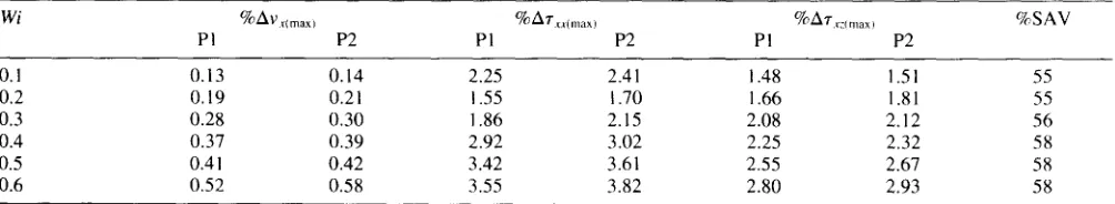
Table 2. M a x i m u m differences of velocity and stresses between solutions obtained from the two methods and analytical solutions for Couette flow using a fine mesh M S H 2 (note that P1 = N T D B E M and P2 = N T D B E M 9 6 )

Wi %AY ~(maxl %Ar~(,,a~l %Arx:, ,,ax~ %SAV

PI P2 PI P2 PI P2

0.1 0.13 0.14 2.25 2.41 1.48 1.51 55

0.2 0.19 0.21 1.55 1.70 1.66 1.81 55

0.3 0.28 0.30 1.86 2.15 2.08 2.12 56

0.4 0.37 0.39 2.92 3.02 2.25 2.32 58

0.5 0.41 0.42 3.42 3.61 2.55 2.67 58

[image:4.576.36.539.102.196.2] [image:4.576.36.538.659.751.2]

(5)

[image:5.576.49.539.98.194.2]

Table 3. Maximum differences of velocity and stresses between solutions obtained from the two methods and analytical solutions for Poiseuille flow using a coarse mesh MSH1 (note that PI = NTDBEM and P2 = NTDBEM96)

Wi

%Avx(max) %ATxx(max) %AT"xz(max ) %SAV

P1 P2 P1 P2 P1 P2

0.1 1.43 1.54 1.10 1.05 1.81 2.01 41

0.2 1.42 1.50 1.05 1.06 1.85 2.2 42

0.3 1.30 1.43 1.02 1.06 1.80 2.3 42

0.4 1.10 1.05 1.04 1.05 1.90 2.3 43

0.5 1.00 0.92 1.02 1.04 1.85 2.1 43

0.6 0.85 0.71 1.00 1.02 1.85 2.1 43

time consuming. Alternatively we can use linear data-fitting techniques by choosing/3, and rn

apriori

and leave o~in to be determined. Zheng e t al. 6"14 and Coleman

et al.~°

obtained good results following this approach. Recommendations for /3~ and r , are also given. In this work rn are chosen to be suitably distributed points in the domain (here we use the points resulted from a typical FE-type discretization). The /3n for each point are chosen to be the average distance from its immediate neighbours multiplied by a weighting factor, and the weighting factor can vary in a range from 0.5 to 2.0 by numerical experiments. ~° In order to obtain accurate solutions, i3~ (or the weighting factor) must be carefully chosen. This matter will be discussed in the next section.

To find oti, one can use either a collocation method or a least-square fitting method. Both of those methods result in a set of linear algebraic equations in which c~i, are unknown. The use of the gaussian distribution as the basis functions makes the system matrix effectively sparse, for which either the Gauss elimination (GE) or an iterative solution method can be used, such as the conjugate gradient method (CGM) 19 which has been known to be more efficient for large systems. The results shown in the next section were obtained with both GE and C G M methods. The differences in the results by the two methods are in the range o f 0 . 0 1 - 0.05%, which must be due to the iterative nature of the C G M method.

5 N U M E R I C A L R E S U L T S

5.1 T e s t p r o b l e m s

In this section we show some test results obtained from the procedure described above. The code was tested in some simple flows (Couette and Poiseuille flows) for which

analytical solutions are known. The pseudo-body force was calculated using gaussian quadrature formulas; 5 the same procedure is adopted here. For each problem a coarse mesh, MSH1 (with 73 boundary nodes and 79 domain nodes) and a fine mesh, MSH2 (with 709 boundary nodes and 1549 domain nodes) were used.

Couette and Poiseulle flows o f an upper-convected Max- well fluid are used to test the program. The boundary conditions for the two flows are illustrated in Figs 1 and 2. The velocity and stress fields are obtained analytically by solving the field equations with appropriate boundary con-

ditions. 21 Field variables are non-dimensionalized

according to

t~ t X'---- X_, u'----U, 7"' 7"

---~' a ---U

7 - -

a

where t is time, x is the position vector, u is the velocity vector, r is the extra stress tensor and ~ is the viscosity. X is the fluid relaxation time, a is a typical length and U is a typical flow speed. Then, for Couette flow, the velocity field v and stress field 7 are given as

V ~

[!

t/p

, 7 ~

L2wi%~

10

For Poiseuille flow, we have

V =

~h 2

~ - ~ ( 1 - z 2)

0

[

2~pWiz 2 0 - z %

0 0

L - Z~p 0 0

[image:5.576.37.540.660.753.2]

In these formulas 5' denotes shear rate,

Wi

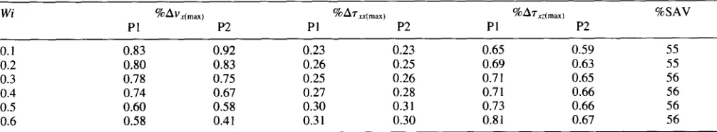
= ~,'i' is the

Table 4. Maximum differences of velocity and stresses between solutions obtained from the two methods and analytical solutions for Poiseuille flow using a fine mesh MSH2 (note that P1 = NTDBEM and P2 = NTDBEM96)

Wi

%Avx(max) °~AT"xx(max ) °~mTxz(max ) %SAV

P1 P2 PI P2 PI P2

0.1 0.83 0.92 0.23 0.23 0.65 0.59 55

0.2 0.80 0.83 0.26 0.25 0.69 0.63 55

0.3 0.78 0.75 0.25 0.26 0.71 0.65 56

0.4 0.74 0.67 0.27 0.28 0.71 0.66 56

0.5 0.60 0.58 0.30 0.31 0.73 0.66 56

(6)

I I I I I

Fig. 3. A refined mesh MSH2 for a square die.

W e i s s e n b e r g number, X is the relaxation time and c~ is the pressure gradient in the direction of the flow (for Poiseuille flow only).

To simplify the test problems we choose in these examples y = l , ~p = 1, c~ = 1, h = 1 and U = 1. The values of /3~ in eqn (14) are chosen via the weighting

-1.5

-2

-2.5

-3

-3.5

-4

NTDBEM-MSH1 NTDBEM96-MSH1 o

NTDBEM-MSH2 K NTDBEM96-MSH2 =

-4.5

-7 -6 -5 -4 -3 -2 -1 0

Iteration(current-last)

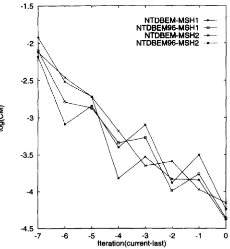
Fig. 4. Rate of convergence (Wiw = 0.225). Note that a CM of O(10 -3 ) is achieved in about five iterations.

8

u) 30

25

20

10

~ITDBEM96-MSH1 ~ITDBEM96-MSH2 ~

~

(a)

0 L i i i i

0.1 0.2 0.3 0.4 0.5 0.6 0.7

Wiw

Fig. 5. Swell ratios as a function of Wiw: (a) across OA; and (b) across OB (see Fig. 3.)

factor, which is 1.0. Although the weighting factor can be chosen in the range from 0.5 to 2.0, it is found that the accuracy o f the solution is sensitive to the choice of this parameter. The best value is in the range o f 0 . 9 - 1 . 1 for Couette and Poiseuille flows. Similar influence of the weighting factor is found in studies by C o l e m a n et aL l° and Jackson 2°. To confirm the accuracy of the programs, studies are carried out with different values o f Wi. For each value o f Wi the convergence measure, which is less than 10 -6 , is obtained after two to three iterations for Couette flow and four to six iterations for Poiseulle flow. The convergence measure (CM) is defined by

1

(u7 - u7

C M = I, I i=1

1 (22)

where ui is t h e / - v e l o c i t y component at a node, N is the total number of nodes, n is the iteration number. Tables 1 - 4 show the m a x i m u m differences in percentage between analytical solutions and those obtained by N T D B E M and NTDBEM96. The times that can be saved by using the new routine (in comparison with the old one) are also presented in the last column o f these tables.

[image:6.576.40.277.72.367.2] [image:6.576.305.533.76.323.2] [image:6.576.43.272.481.728.2]

(7)

[image:7.576.39.536.99.187.2]

Table 5. Die shape relative to a required square extrudate as a function of

Wi

in percentage (note that the data for NTDBEM are

from Tran-Cong and Phan-Thien 15)

Wi Across OB Across OA

W/w

NTDBEM NTDBEM96 NTDBEM NTDBEM96

0.05 0.1124 - 19.3 - 19.0 + 1.9 + 1.7

0.10 0.2248 - 21.0 - 20.5 + 0.8 + 0.5

0.15 0.3372 - 23.8 - 23.4 - 1.3 - 1.8

5.2 Extrusion problems

In this section we show some results o f study o f extrusion o f M P T T fluid through a square die. The results are c o m p a r e d with those obtained b y Tran-Cong and Phan-Thien 5'~5 for a coarse mesh MSH1 (with 166 boundary nodes and 349 volume nodes discretization). The boundary conditions are as follows. At the die inlet, a Newtonian velocity profile is prescribed and the flow is allowed to develop downstream before reaching the die exit. The free surface o f the extrudate downstream from the die exit is traction-free. A no-slip condition is assumed on the die walls. Extrudate swell is the

principal phenomenon under investigation here. For

geometry other than circular or planar, 'swelling ratio' is not uniquely defined. In the present problem, a typical ratio o f the distance from the centreline to the extrudate surface over the corresponding distance from the centreline to the die surface is defined as the local swelling ratio. F o r the square die, two typical ratios are reported here. One is measured along OA and the other is along OB as shown in Fig. 3.

W e also use Wiw (the W e i s s e n b e r g n u m b e r based on a wall shear rate at a point far upstream, Wiw -~ 2.25 Wi for a square die) for convenience. W i t h a refined mesh M S H 2 (with 544 boundary nodes and 1794 d o m a i n nodes) shown in Fig. 3 it is difficult to carry on the analysis with N T D B E M because o f high d e m a n d o f CPU time (it takes from 1 5 - 2 0 h to finish one iteration on a Silicon Graphics Indigo2 machine with a MIPS R4400 C P U and 128 M b y t e s o f R A M ) . The program N T D B E M 9 6 , with the new routine

1.3 1.2 1.1

1

0.9 0.8 0.7

0.6

I

0.5 0.4 0.3

0.2 ÷

0.4

I I i I i

T x x T z ~

I / x

0.6 0.8 1 1.2 1.4

Weighting factor 1.6

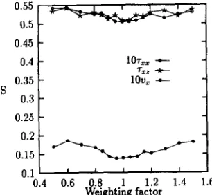
Fig. 6. Numerical solution 'S' for Couette flow (Wi = 0.1) as a function of weighting factor. Note that the solutions are taken at

the node labelled as A in Fig. 1.

for the approximation o f the d o m a i n integral, gives the solutions in a relatively short time. Fig. 4 shows the rate o f convergence o f the extrusion analysis with Wiw = 0.225 using both N T D B E M and N T D B E M 9 6 . The swelling ratio as a function o f Wiw is presented in Fig. 5. As can be seen from the figure, the results differ by less than 1.0% (MSH1) and 0.3% (MSH2). Note that with the finer mesh used here (MSH2) we stop the simulation using N T D B E M (i.e. the old implementation) after the first three Wis values because o f high CPU demand. W i t h the present improved implementation (NTDBEM96), we could continue the simulation at a much lower cost. However, we encounter a p r o b l e m o f convergence. It appears that the problem fails to converge at a lower Wi number when a finer mesh is used. For example, with MSH1, N T D B E M 9 6 converges up to

Wiw = 1.01 and only up to Wiw = 0.68 with MSH2. This is a separate issue which will be further investigated.

The weighting factor in this problem is chosen to be 0.6 which is the mid-point o f the best range o f 0 . 5 5 - 0 . 7 5 found experimentally for the extrusion problem. The time required to finish every iteration by both programs is recorded. The C P U time which the new routine can save is 5 5 - 6 0 % for the coarse mesh MSH1 and 6 3 - 7 0 % for the fine mesh MSH2. F r o m results o f the test problems (Tables 1 - 4 ) and the extrusion problems it is found that relatively more time (i.e. higher percentage) is saved as meshes are refined, which is advantageous.

Table 5 shows some indicative results obtained by using the same procedure for an inverse p r o b l e m (the results are in

0.55 0.5 0.45 0.4 0.35 0.3 0.25 0.2 0.15 0.1

0.4

lOr~ --- 10v~ -4--

I I I I I

0.6 0.8 1 1.2 1.4 1.6

Weighting factor

Fig. 7. Numerical solution 'S' for Poiseuille flow (Wi = 0.1) as a function of weighting factor. Note that the solutions are taken at

[image:7.576.336.489.568.709.2] [image:7.576.70.228.570.710.2]

(8)

comparison with those obtained by Tran-Cong ~6 and Tran- Cong and Phan-Thien 15 using quadrature formulas). In this problem it is required to compute the die geometry that will produce a given extrudate geometry (square cross-section in this case). This is a typical engineering problem which is still largely solved by trial and error experimentation. Given that the extrudate geometry is fixed (in contrast to the direct extrusion problem), the values shown in Table 5 are measures of the computed die geometry relative to the extrudate. Negative values indicate that the required die is smaller than the extrudate which is consistent with the die swell phenomenon, especially at higher Wi numbers. At lower Wi numbers when the material behaviour is close to Newtonian, we observe some local contraction of the extrudate as indicated by the positive values shown in the table. The time saving in this problem is almost the same as in the direct extrusion problem.

5.3 The choice of the weighting factor

As mentioned earlier, the choice of the weighting factor is a difficult problem which is determined by appropriate numerical experiments. We note the following:

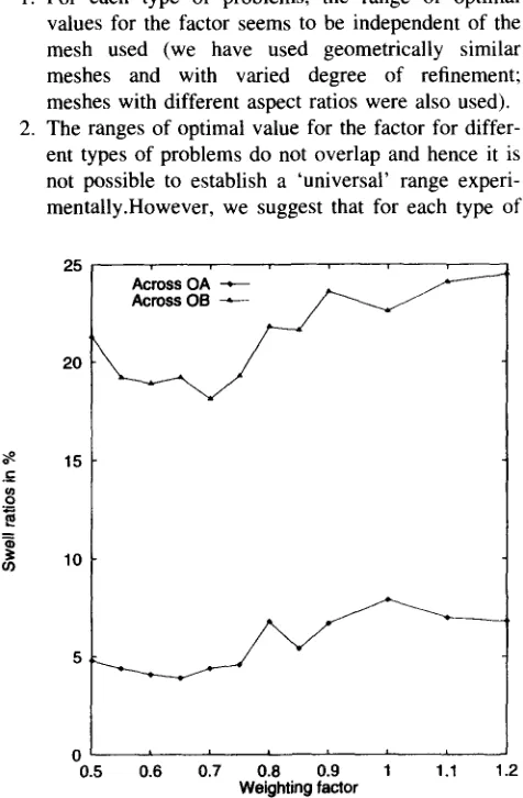
1. For each type of problems, the range of optimal values for the factor seems to be independent of the mesh used (we have used geometrically similar meshes and with varied degree of refinement; meshes with different aspect ratios were also used). 2. The ranges of optimal value for the factor for differ-

ent types of problems do not overlap and hence it is not possible to establish a 'universal' range experimentally.However, we suggest that for each type of

problem, we might be able to establish a valid range for the weighting factor for subsequent routine analyses. The basis for this idea is shown in Figs 6 - 8 where it can be seen that approximately correct solutions correspond to a 'flat' region in the plot of numerical solutions vs weighting factor. Furthermore, it appears that this region is the neighbourhood of the extremum of the numerical solutions with respect to the weighting factor. The optimum value for the weighting factor can then be chosen to be roughly in the middle of this 'flat' region, which has been done in this study.

6 C O N C L U D I N G R E M A R K S

Routine engineering analysis of three-dimensional polymer extrusion process, especially the inverse process where a die geometry is to be computed for a given extrudate profile, is practically very important in reducing the high cost involved (trial and error die manufacturing and long lead- time). Direct BEMs have been successfully applied to this kind of analysis. S'15'16 However, more efficient techniques are required, and provided here in this work, in order to analyse larger problems. The results reported here show that the efficiency of the method has been significantly improved. More importantly, efficiency gain is greater for larger problems. This work has demonstrated that larger practical plastic extrusion analyses can be done on desktop machine (a Silicon Graphics Indigo2 with a MIPS R4400 CPU and 128 Mbytes of RAM was used in this work).

25

2 0

o~ 15 ._.q.

~= 1 0

Across O A --,,---

0 I I I i I L

0.5 0.6 0.7 0.8 0.9 1 1.1 Weighting factor

Fig. 8. Numerical solution for the extrusion problem at Wi,~ =

0.225. Note that the labels OA and OB are defined in Fig. 3.

A C K N O W L E D G E M E N T S

This work is supported by Australian Research Council Grants. T. Nguyen-Thien is supported by an AusAID Scholarship. This support is greatfully acknowledged. We would like to thank the referees for their helpful comments.

R E F E R E N C E S

I. Bush, M.B. & Tanner, R.I. Numerical solution of viscous flows using integral equation method. International Journal

of Numerical Methods of Fluids, 1983, 3, 71-92.

2. Bush, M.B. & Phan-Thien, N. Three dimensional viscous flow with a free surface: flow out of a long square die. Jour-

nal of Non-Newtonian Fluid Mechanics, 1985, 18, 211-218.

3. Bush, M. The application of boundary element method to some fluid mechanics problems, Ph.D. Thesis, The Univer- sity of Sydney, Australia, 1983.

4. Bush, M. Prediction of polymer melt extrudate swell using a differential constitutive model. Journal of Non-Newtonian

Fluid Mechanics, 1989, 31, 179-191.

[image:8.576.37.275.365.728.2]

(9)

6. Zheng, R., Coleman, C.J. & Phan-Thien, N. A boundary element approach for non-homogenous problems. Computa- tional Mechanics, 1991, 7, 279-288.

7. Banerjee, P.K., Ahmad, S. & Wang, H.C. A new BEM For- mulation for the acoustic eigenfrequency analysis. Inter- national Journal of Numerical Methods in Engineering, 1988, 26, 1299-1309.

8. Patridge, P. W., Brebbia, C. A. & Wrobel, L.C. The Dual Reciprocity Boundary Element Method. Computational Mechanics Publication and Elsevier Applied Science, London, 1990.

9. Tang, W. Transforming Domain into Boundary Integrals in BEM. Springer, New York, 1988.

10. Coleman, C.J., Tullock, D. & Phan-Thien, N. An effective boundary element method for inhomogeneous partial difer- ential equations. ZAMP, 1991, 42, 730-745.

11. Ingber, M.S. & Phan-Thien, N. A boundary element approach for parabolic differential equations using a class of particular solutions. Applied Mathematical Modelling,

1992, 16, 124-132.

12. Zheng, R. & Phan-Thien, N. Transforming the domain integrals to the boundary using approximate particular solutions: a boundary element approach for non-linear problems. Applied Numerical Mathematics, 1992, 10, 435-445. 13. Powell, M. J. D. The theory of radial basis fuction

approximation in 1990, In Advances in Numerical Analysis, ed. W. Light. Clarendon, Oxford, 1991, pp. 105-209. 14. Zheng, R., Phan-Thien, N. & Coleman, C.J. A boundary

element approach for non-linear boundary value problems. Computational Mechanics, 1991, 8, 71-86.

15. Tran-Cong, T. & Phan-Thien, N. Profile extrusion and die design for viscoelastic fluids. In Simulation of Materials Pro- cessing: Theory, Methods and Applications, ed. S-F. Shen, P. Dawson, Balkema. Rotterdam, 1995, pp. 183-189. 16. Tran-Cong, T. Boundary element method for some three-

dimensional problems in continuum mechanics. Ph.D. thesis, The University of Sydney, Sydney, 1989.

17. Parton, V. Z. & Perlin, P. I. Mathematical Methods of the Theory of Elasticity. Mir, Moscow, 1984.

18. Phan-Thien, N. & Kim, S. Microstructure in Elastic Media Principle and Computational Methods. Oxford University Press, Oxford, 1994.

19. Stoer, S. & Bulirsch, R. Introduction to Numerical Analysis. Springer, New York, 1976.

20. Jackson, I.R.H. Radial basis functions: a survey of new

results. In The Mathematics of Surfaces I11, ed.

D. C. Handscomb. Oxford University Press, Oxford, 1989, pp. 115-133.