Stochastic simulation for planning optimal log hauling operations

(1)

OPTIMAL LOG HAULING OPERATIONS

by

NEIL ROSS ADA

A thesis submitted for the degree of Doctor of Philosophy of the Australian National University.

(2)

ORIGINALITY OF THESIS

(3)

Log transport operations are becoming more complex and there are increasing opportunities to apply Operations Research techniques to their planning and evaluation. A stochastic simulation model representing log hauling operations was developed and statistically validated in a case study of haulage to a centralized mill from several forest blocks.

Theoretical distributions are presented for the elements of the log hauling cycle and the loadweights of the trucks in the case study. The results of a separate study of the frequency and duration of log truck breakdowns are also presented.

The simulation model was used in conjunction with a mixed- integer programme to plan optimal log hauling operations for delivery of 8 000 tonnes of wood per week to a central mill from nine forest blocks. The simulation studies shewed substantial yearly savings with increases in gross vehicle weight limits, adoption of double shifts for trucks and loaders and reduction in the loading times. The results of an evaluation of leasing or purchasing for equipment procurement is also presented. The simulation studies indicated that leasing was more cost effective.

(4)

I wish to thank my supervisor Don Stodart for his interest and guidance throughout the study. His criticisms and advice are most appreciated. I would also like to thank Ken Groves for his advice and Brian Turner for his advice since arriving in the department and his criticism of the draft thesis. The following also deserve mention:

- Professor D.M. Griffin and the Forestry department for the provision of facilities to carry out the study.

- Professor I.S. Ferguson for his helpful advice at the beginning of the stud/’.

- Joe Miles and Terry Johnson for their invaluable advice and assistance in the use of the computing facilities. The Department of Primary Industry for the Postgraduate Research Award which financed the project.

- Australian Newsprint Mills Ltd and its personnel, especially Curly Humphries and Terry Beath for providing access to records and advice.

- Nev Zealand Forest Products Pty. Ltd. for providing access to company records on log truck breakdowns.

- Ian MacArthur of the Harvesting Research Group, Division of Forest Research, CSIRO for advice on truck costs.

- Staff of the Forestry department, particularly Paula Reid for library assistance and tete-a-tetes and Liz Robinson, Beverly Hawkins and Audrey Maher in the front office for a million and one things.

(5)

TABLE OF CONTENTS

Page

ABSTRACT iii

ACKNOWLEDGEMENTS iv

TABLE OF CONTENTS v

LIST OF TABLES xii

LIST OF FIGURES xviii

LIST OF PHOTOGRAPHS xx

LIST OF MAPS xx

LIST OF APPENDICIES xxi

CHAPTER 1 THE TRANSPORTATION OF LOGS 1

1.1 INTRODUCTION 1

1.2 COST PARAMETERS FOR LOG HAULAGE 3

1.2.1 Vehicle Costs 4

1.2.2 Loads Carried by Trucks 4

1.2.3 Speed of Trucks 6

1.2.4 Haul Distance 6

1.2.5 Delays and Breakdowns to Equipment 7

1.2.6 Managerial Efficiency 7

1.3 FORMULATION OF THE STUDY 8

1.3.1 Aims 8

1.3.2 The Abstract Model 9

1.4 OPERATIONS RESEARCH 10

1.4.1 Introduction 10

1.4.2 Classification of Models 11

1.4.3 Simulation 14

(6)

1.5 HARVESTING AND TRANSPORT SIMULATION MODELS 18 1.5.1 Harvesting Simulation Models 18

1.5.2 Transport Models 19

1.6 THE CONCEPTUAL MODEL 20

1.6.2 The Dynamics of Log Haulage Systems 22

1.7 THE CASE STUDY 26

1.7.2 The ANM Operations at Albury,

Nev South Whies 29

1.7.2.1 The overall system 29

1.7.2.2 The harvesting system 31

1.7.2.3 The loading system 32

1.7.2.4 The hauling system 33

1.7.3 The Study Approach 37

CHAPTER 2 DATA COLLECTION AND ANALYSIS 38

2.2 DATA COLLECTION 39

2.2.1 Sources of Data 39

2.2.1.1 The truck drivers 39

2.2.1.2 Truck tachographs 40

2.2.1.3 The loader operators 40

2.2.1.4 ANM weighbridge records 40

2.2.2 Data Collection and Compilation 41

2.3 DATA ANALYSIS 42

2.3.1 Time in the Mill Yard by Trucks 45 2.3.2 Travel Times by Trucks Between the

Landing and the Mill 52

2.3.3 Loading Times for Trucks 62 2.3.4 Travel Times by Trucks Between the

Mill and the Landing 64

2.3.5 Frequency and Duration of Breakdowns

to Trucks 66

2.3.6 Loadweights of Trucks 67

2.4 COSTS OF LOADERS AND TRUCKS 72

2.4.1 Introduction 7 2

2.4.2 Costs of Equipment 74

2.4.2.1 Owning costs 74

2.4.2.2 Operating costs 78

(7)

CHAPTER 3 FREQUENCY AND DURATION OF LOG TRUCK BREAKDOWNS 80

3.2 DATA COLLECTION 81

3.3 DESCRIPTIVE STATISTICS OF FREQUENCY AND

DURATIONS OF BREAKDOWNS 82

3.3.1 Descriptive Statistics for Age

Based Data 83

3.3.2 Descriptive Statistics for Distance

Based Data 85

3.4 FITTING PROBABILITY DENSITY FUNCTIONS FOR

INTERVALS BETWEEN AND DURATIONS OF BREAKDOWNS 89 3.4.1 Distributions for the Intervals

Between Breakdowns (hours) 89 3.4.2 Distributions for the Durations of

Breakdowns 91

3.5 TIME DEPENDENCE OF THE INTERVALS BETWEEN

BREAKDOWNS (HOURS) 97

3.5.1 Testing for Time Dependence 98

3.6 REVIEW 101

CHAPTER 4 THE SIMULATION MODEL 106

4.1 INTRODUCTION 106

4.2 CHOICE OF LANGUAGE 109

4.3 THE CORE MODEL AND ITS ANCILLARY ROUTINES 111

4.3.1 The Core Model 111

4.3.1.1 Morning start up subsysten 114 4.3.1.2 Close weighbridge subsystem 116

4.3.1.3 Loader night subsysten 116

4.3.1.4 Landing subsystem 118

4.3.1.5 Mill subsystem 118

4.3.1.6 Scheduler subsystem 121

4.3.1.7 Home subsysten 123

4.3.2 Ancillary Routines 123

4.3.3 Control Checks in the Model 124 4.4 APPLICATION OF THE CORE MODEL TO

THE ANM SYSTEM 124

(8)

4. 5 . 1 D a t a I n p u t s f r o m F i e l d O p e r a t i o n s 127 4 . 5 . 2 D a t a I n p u t s as M a n a g e r i a l S p e c i f i c a t i o n s 127 CHAPrER 5 V E R I F I C A T I O N A N D V A L I D A T I O N O F T H E

S I M U L A T I O N M O D E L 129

5.1 INrRODUCTION 129

5.2 V E R I F I C A T I O N O F T H E C O R E M O D E L 136 5.2.1 P s e u d o - r a n d o m N u m b e r G e n e r a t o r 136 5 .2.2 S t r u c t u r e o f t h e M o d e l 136 5.2.3 D a t a V e r i f i c a t i o n 137 5.3 V A L I D A T I O N O F T H E M O D E L 140 5.3.1 S t a r t i n g C o n d i t i o n s f o r S i m u l a t i o n Runs 1 40 5.3.2 D a t a P e r i o d s f or V a l i d a t i o n 141

5 .4 P E R I O D V A L I D A T I O N 141

5.4.1 D a t a 141

5 .4.1.1 D a y s w o r k e d b y l o a d e r s 142 5 . 4 . 1 . 2 H o u r s w o r k e d b y l o a d e r s 142 5 . 4 . 1 . 3 M o v e m e n t o f l o a d e r s 143 5 . 4 . 1 . 4 N u m b e r o f t r u c k s 145 5.4.2 T h e A s s u m p t i o n s for t h e P e r i o d

V a l i d a t i o n 146

5.4.3 O u t p u t s o f t h e M o d e l R u n s for

t h e P e r i o d V a l i d a t i o n 146 5 . 4 . 4 R e s u l t s for t h e P e r i o d M o d e l

V a l i d a t i o n 149

5 . 4.4.1 N o v e m b e r 1982: p e r i o d I 149 5 . 4 . 4 . 2 F e b r u a r y 1983: p e r i o d II 155 5 . 4.4.3 J u n e 1983: p e r i o d III 162

5 . 4 . 4 . 4 D i s c u s s i o n 168

5.5 D A I L Y V A L I D A T I O N 170

5.5.1 I n t r o d u c t i o n 170

5.5.2 C o m p a r i s o n o f t h e R e a l a n d

S i m u l a t e d D a i l y P e r f o r m a n c e 171 5 . 5.2.1 N o v e m b e r 2 2 n d 1982 171 5 . 5 . 2 . 2 F e b r u a r y 1 1 t h 1 9 8 3 175 5.5 . 2 . 3 J u n e 2 n d 1983 175 5.5.3 R e v i e w o f D a i l y V a l i d a t i o n 176

5.6 C O N C L U S I O N 178

C H A P T E R 6 E X P E R I M E N T A L A P P L I C A T I O N O F T H E S I M U L A T I O N M O D E L 179

(9)

6.2 OPTIMIZATION OF SIMULATED SYSTEMS 182 6.2.1 Mathematical Programming 183

6.2.1.1 Linear programming 183

6.2.1.2 Nonlinear programming 186

6.3 OUTLINE OF THE EXPERIMENTAL STUDIES 187

6.3.1 Experimental Design 187

6.3.2 Simulation Methodology 191

6.3.3 Assumptions and Constraints 193 6.3.4 Programming and Optimization Procedures 195 6.4 EXPERIMENT Is STUDIES OF GROSS VEHICLE WEIGHTS 200

6.4.1 Aim 200

6.4.2 38 Tonne Gross Vehicle Weight Limit 200

6.4.2.1 Introduction 200

6.4.2.2 Results for four loaders 201 6.4.2.3 Results for three loaders 201 6.4.3 40 Tonne Gross Vehicle Weight Limit 206

6.4.3.1 Introduction 206

6.4.4.1 Introduction 207

6.4.5.1 Introduction 208

6.4.5.2 Results for four loaders 209 6.4.5.3 Results for three loaders 209 6.4.6 Summary of Gross Vehicle Weight Results 209 6.4.7 Review of Gross Vehicle Weight Results 209 6.4.7.1 The effect of gross vehicle weights

on loading and hauling costs 209 6.4.7.2 Three loader versus four loader

operations 215

6.4.7.3 Truck utilization 216

6.4.7.4 Allocation of trucks to loaders 217 6.5 EXPERIMENT 2: EVALUATION OF DOUBLE SHIFTS FDR

BOTH LOADERS AND TRUCKS 217

6.5.1 Aim 217

6.5.2 Methodology 218

6.5.3 Simulation of Two Separate Twelve

Hour Shifts 220

6.5.3.1 Introduction 220

6.5.3.2 Results for twc twelve hour shifts 221 6.5.4 Simulation of Two Overlapping Shifts 222

(10)

6 . 5 . 4 . 2 R e s u l t s for t h e o v e r l a p p i n g shi f t s 2 22 6.5.5. S u m m a r y o f D o u b l e S h i f t R e s u l t s 222 6 . 5 . 6 R e v i e w o f D o u b l e S h i f t R e s u l t s 223 6 . 5 . 6 . 1 T h e e f f e c t o f d o u b l e s h i f t s o n

l o a d i n g a n d h a u l i n g c o s t s 223 6 . 5 . 6 . 2 L o a d e r u t i l i z a t i o n 223 6 . 5 . 6 . 3 T r u c k u t i l i z a t i o n 226 6 . 6 E X P E R I M E N T 3: A S S E S S M E N T O F T H E E F F E C T O F

R E D U C T I O N S IN L O A D I N G T I M E S 227

6 .6.1 I n t r o d u c t i o n 227

6 . 6 . 2 M e t h o d o l o g y 228

6 . 6 . 3 S i m u l a t e d S y s t e m P e r f o r m a n c e w i t h a

M e a n L o a d i n g T i m e o f T w e n t y M i n u t e s 2 2 8 6 . 6 . 3 . 1 R e s u l t s for f o u r l o a d e r s 228 6 . 6 . 3 . 2 R e s u l t s for t h r e e l o a d e r s 229 6 . 6 . 4 S i m u l a t e d S y s t e m P e r f o r m a n c e w i t h a

M e a n L o a d i n g T i m e o f S i x t e e n M i n u t e s 2 29 6 . 6 . 4 . 1 R e s u l t s for f o u r l o a d e r s 229 6 . 6 . 4 . 2 R e s u l t s for t h r e e l o a d e r s 229 6 . 6 . 5 S u m m a r y o f L o a d T i m e R e s u l t s 230 6. 6 . 6 R e v i e w o f L o a d T i m e R e s u l t s 230 6 . 6 . 6 . 1 E f f e c t o f r e d u c i n g l o a d t i m e s o n

h a u l a g e c o s t s 2 30

6 . 6 . 6 . 2 F o u r l oaders v e r s u s t h r e e loaders 235 6.6 . 6 . 3 T r u c k u t i l i z a t i o n 236 6.7 R E V I E W (DF E X P E R I M E N T A L S I M U L A T I O N R E S U L T S 236 C H A P T E R 7 A C O M P A R A T I V E C A S E S T U D Y O F L E A S I N G A N D

P U R C H A S I N G L O G T R U C K S 2 38

7.1 I N T R O D U C T I O N 2 38

7.2 M E T H O D O L O G Y 238

7.3 R E S U L T S 241

7 .3.1 L e a s i n g o f T r u c k s t o S e r v i c e t h e

S h e l l e y F o r e s t B l o c k 241 7 .3.2 P u r c h a s i n g o f T r u c k s t o S e r v i c e the

S h e l l e y F o r e s t B l o c k 241 7 .3.3 L e a s i n g o f T r u c k s t o S e r v i c e t h e

B a t l c w - 1 F o r e s t B l o c k 243 7 . 3 . 4 P u r c h a s i n g o f T r u c k s t o S e r v i c e t h e

B a t l c w - 1 F o r e s t B l o c k 243

7 . 4 R E V I E W 245

C H A P T E R 8 R E V I E W 251

(11)

8.3

8.4 8.5

REFERENCES

8.2.1 The Conceptual Model 252

8.2.2 Data Collection 253

8.2.3 Fitting Probability Density

Functions 254

8.2.4 Choice of Language 254

8.2.5 Validation of Log Transport

Simulation Models 255

8.2.6 Optimization of Log Hauling

Operations 256

8.2.7 Summary 256

APPLICATIONS OF THE MODEL 257

8.3.1 Introduction 257

8.3.2 Operational Experiments 258

8.3.2.1 Gross vehicle weight limits 258 8.3.2.2 Double shifts for trucks and

loaders 253

8.3.2.3 Load times 259

8.3.2.4 Review 260

8.3.3 Equipment Procurement Procedures 261

MODELLING LOG TRUCK BREAKDOWNS 262

FURTHER APPLICATIONS OF THE MODEL 263

8.5.1 Introduction 263

8.5.2 Nav Applications 264

8.5.3 Future Research 265

268

(12)

LIST OF TABLES

Number Title Page

1.1 Costs of log haulage from ACT forests under

two load limits 5

1.2 Quantifiable properties of the truck fleet

in a generalised hauling system 25

1.3 Quantifiable properties for loaders and

unloaders in a generalised hauling system 27 2.1 Goodness of fit statistics for the best

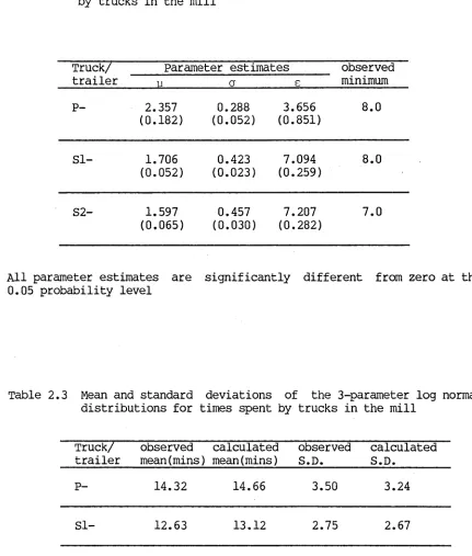
distributions for time spent by trucks in the mill 48 2.2 Parameter estimates (standard errors in

brackets) for the 3-parameter log normal distribution representing times spent by

trucks in the mill 51

2.3 Mean and standard deviations of the 3-parameter log normal distributions for

times spent by trucks in the mill 51

2.4 Goodness of fit statistics for the best distributions for travel times from forest

blocks to the mill 57

2.5 Parameter estimates (standard errors in brackets) for the 3-parameter log normal distribution

for travel times fron forest blocks to the mill 60 2.6 Means and standard deviations of the 3-parameter

log normal distibutions for travel times from

forest blocks to the mill 61

2.7 Analysis of variance for times for loading

trucks at landings under four loaders 63 2.8 Times for loading trucks at landings 63 2.9 Cycle times and travel times to and from

the mill for forest blocks 65

2.10 Goodness of fit statistics for nett loadweights

by truck/trailer combinations 71

2.11 Parameter estimates (standard errors in brackets) for the normal and 3-parameter log normal distributions for nett loadweights

of truck/trailer combinations 73

(13)

3-parameter log normal distributions for nett

loadweights of truck/trailer combinations 73 2.13 Summary of costs of trucks and loaders adopted

for the simultion studies 77

3.1 Descriptive statistics for durations of

breakdowns of two age classes of trucks 84 3.2 Descriptive statistics for intervals between

breakdowns of two age classes of trucks 86 3.3 Descriptive statistics for durations of

breakdowns of three classes of distance

travelled by trucks 87

3.4 Descriptive statistics for intervals between breakdowns of three classes of distance

3.5 Goodness of fit statistics for intervals between breakdowns of three classes of

distance travelled by trucks 92

3.6 Parameter estimates (standard errors in brackets) of three distributions of the intervals between breakdowns for three classes of distance

3.7 Goodness of fit statistics for durations of

breakdowns for three classes of distance travelled

by trucks 95

3.8 Parameter estimates (standard errors in brackets) of the 3-parameter log normal distribution

for the durations of breakdowns for three classes

of distance travelled by trucks 96

3.9 Serial and ranked serial coefficients for the

intervals between breakdowns for each truck 101 5.1 Comparison of the means and standard deviations

used as input for the distribution and the simulated output for the time spent by trucks

in the mill 138

5.2 Comparison of the means and standard deviations used as input for the distribution and the

simulated output for nett loadweight of trucks 138 5.3 Comparison of the means and standard deviations

used as input for the distribution and the

(14)

5.4 Comparison of the empty factors and the means and standard deviations used as input for the distribution and the simulated output for

travel-full times 139

5.5 Results for period I validation: number of loads

delivered per day 150

5.6 Results for period I validation: number of

tonnes delivered per day 150

5.7 Results for period I validation: number of

trucks used per day 151

5.8 Results for period I validation: hours worked

by trucks per day 151

by loader 71 per day 152

5.13 Results for period I validation: percentage of

loads delivered from NSW and Victoria 154 5.14 Results for period II validation: number of loads

5.15 Results for period II validation: number of

5.16 Results for period II validation: number of

5.17 Results for period II validation: hours worked

(15)

5.22 Results for period II validation: percentage of

loads delivered from NSW and Victoria 160 5.23 Results for period III validation: number of loads

5.24 Results for period III validation: number of

5.25 Results for period III validation: number of

5.26 Results for period III validation: hours worked

5.31 Results for period III validation: percentage

of loads delivered from NSW and Victoria 167 5.32 Daily validation November 22nd 1982: comparison

of loads delivered and hours worked 172

5.33 Daily validation February 11th 1983: comparison

of loads delivered and hours worked 173

5.34 Daily validation June 2nd 1983: comparison of

loads delivered and hours worked 174

5.35 Number of occurrences for various differences between actual and simulated loads delivered

per day 177

5.36 Number of occurrences for various differences

(16)

6.3 Summary program tableau for optimization model 199 6.4 Results for 38 tonne gross vehicle weight

experiment using four loaders 202

6.5 Operating statistics of trucks and loaders for the 38 tonne gross vehicle weight experiment

using four loaders 203

6.6 Results for 38 tonne gross vehicle weight

experiment using three loaders 204

6.7 Operating statistics of trucks and loaders for the 38 tonne gross vehicle weight experiment

using three loaders 205

6.8 Simulated weekly wood deliveries and costs over a five day period for the gross vehicle weight

experiment 210

6.9 Simulated utilization of loaders over a five day

period for the gross vehicle weight experiment 211 6.10 Simulated utilization of trucks over a five

day period for the gross vehicle weight

experiment 212

6.11 Loader schedule and locations for the two

separate twelve hour shifts 221

6.12 Simulated weekly wood deliveries and costs over a five day period for the double shift experiment

using three loaders 224

6.13 Simulated utilization of loaders over a five day period for the double shift experiment using

three loaders 224

6.14 Simulated utilization of trucks over a five day period for the double shift experiment using

three loaders 225

6.15 Simulated weekly wood deliveries and costs over

a five day period for the load time experiment 231 6.16 Simulated utilization of loaders over a five

day period for the load time experiment 232

6.17 Simulated utilization of trucks over a five day period for the load time experiment

7.1 Leasing and depreciation costs per day with

(17)

various hours travelled by trucks

7.2 Cost per tonne of wood delivered from the Shelley and Batlcw-1 forest blocks under specified quotas

7.3 Comparison of the cost per tonne of delivered wood for various tonneage quotas and numbers of trucks frcm two forest blocks

246

248

(18)

LIST OF FIGURES

Number Title Page

1.1 Schematic diagram of a generalised hauling system 24 1.2 Sequential processes and exogenous noncontrollable

parameters of the conceptual model 28

2.1 Average time spent by trucks in the mill for one load for the three truck/trailer combinations for

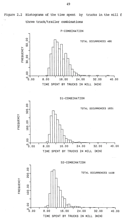
each week of the data collection period 47 2.2 Histograms of the time spent by trucks in the

mill for the three truck/trailer combinations 49 2.3 Location of the compartments for which data

existed and delineation of forest blocks 53 2.4 Histograms of travel times to the mill 56 2.5 Average nett loadweights of each truck/trailer

combination for each week of the data

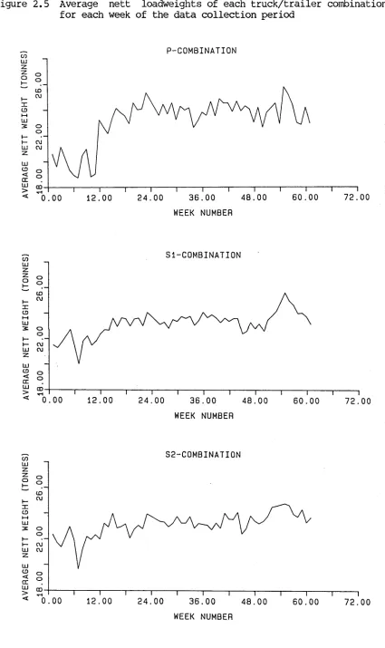
collection period 68

2.6 Histograms of the gross vehicle weights for

each truck/trailer combination 70

2.7 Economic life of a truck 75

3.1 Histrograms of the intervals between breakdowns (grouped data) for short, medium and long classes

of distance travelled by trucks 90

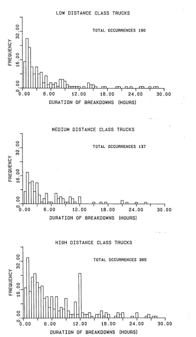
3.2 Histograms for the durations of breakdowns for short, medium and long classes of distance travelled

by trucks 94

3.3 Cumulative number of breakdowns against the

cumulative number of hours worked for each truck 100 3.4 Histograms for the intervals between breakdowns

for short, medium and long classes of distance

travelled by trucks 103

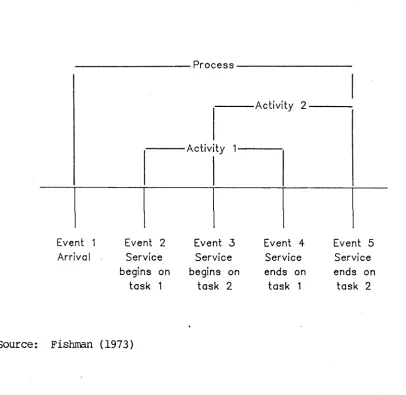
4.1 The relationships between the event, process and activity oriented mechanisms for scheduling

the next event 108

(19)

4.5 Flowchart of the loader night subsystem 117

4.6 Flowchart of the landing subsystem 119

4.7 Flowchart of the mill subsystem 120

4.8 Flowchart of the scheduler subsystem 122

6.1 Simulated total weekly cost against the gross

vehicle weight allowed 214

6.2 Simulated costs per tonne of wood against

the gross vehicle weight allowed 214

6.3 Simulated total weekly cost against the mean

time to load a truck 234

6.4 Simulated costs per tonne of wood against the mean

time to load a truck 234

7.1 Cost per tonne of wood delivered from the Shelley

forest block under the leasing systan for trucks 242 7.2 Cost per tonne of wood delivered from the Shelley

forest block under the purchasing system for trucks 242 7.3 Cost per tonne of wood delivered fron the Batlcw-1

forest block under the leasing system for trucks 244 7.4 Cost per tonne of wood delivered from the Batlcw-1

(20)

LIST OF PHOTOGRAPHS

Plate Title Page

1.1 A 410 Prentice loader 34

1.2 A prime mover with a tri-axle skeletal trailer 36

1.3 A prime mover with a pig trailer 36

LIST OF MAPS

1.1 The area of supply for the ANM mill 30

(21)

LIST OF APPENDICES

2.1 Forms distributed to loader operators and

truck drivers 278

2.2 List of distributions fitted to the data 281

2.3 Mean and standard deviation of the 2- and

3-parameter log normal distributions 282

3.1 Costs for trucks and loaders 283

5.1 Verification of a check run 285

5.2 Listing of the model as used in period validation 288

5.3 Example of a data deck as used in period validation 305

5.4 Comparison of the actual and simulated performance

for the daily validation 309

6.1 Listing of the model as used in experiments 361

6.2 Example of a data deck used in experiments 373

6.3 Determination of sample size 377

(22)

THE TRANSPORTATION OF LOGS

1.1 INTRODUCTION

Nowadays, transport of logs throughout Australia is almost universally by road. It was not of course always so and without doubt, changes and developments that can now be appreciated in an historical perspective will continue to be part of future log haulage systems.

In the early part of the century, sawmills were located as close as possible to the forests to minimize the haulage distance. Bullock teams were commonly used to haul logs from the forest to the mill, sometimes for distances up to 11 kilometres (Simmons 1977). Draught horses with their greater strength, intelligence and more amicable disposition were also used, particularly in hauling the more valuable wood. Bullocks and horses were still used until recently in some parts of New South Wales, because of low volumes of timber per hectare and the small size of the harvesting and transport operations. Horses were used in many parts of the Cypress pine areas of Barradine district while the crack of the bullock whip was heard until 1974 at Bulahdelah (Golding 1974).

(23)

down the rivers and lakes to the coastal ports of Tea Gardens and Port Stephens. The punts were too slow however, and the paddle wheel driven droghers replaced them. Larger loads were carried by the droghers which, since they were equipped with cranes, were not dependent on port facilities as were the punts (Simmons 1977). While the boats provided a ready second phase of transport there were many forests which relied on horses and bullocks to haul directly to the mill.

After the closer forests had been logged and haul distances were beyond the animals' endurance, other hauling systems such as tramways were developed. Initially, the trolleys that carried the logs were pulled by horses along steel capped wooden rails, but as the distance from the mill to the accessible timber increased, a light locomotive running on steel rails was found to be economic. These railway lines extended several kilometres into the forest and were fed directly by bullock teams or winches driven by a steam donkey engine (Johnson 1980).

(24)

Since the first motorised trucks were introduced during the i930's, there has been a steady improvement in their power and performance (Golding 1974 and Johnson 1980) and the modern truck, capable of hauling large loads at high speeds, is now the most efficient for hauling from most landings to mills. There has also been a trend for amalgamation of small individual haulage operations with increasing truck fleet sizes.

The increasing fleet sizes have brought the need for new management techniques. This study is concerned with this need and seeks to make a contribution to the development of techniques to improve the management and operation of truck fleets.

1.2 COST PARAMETERS FOR LOG HAULAGE

In Australia, the transportation of logs has always been a major component of the cost of delivering wood to processing plants. The haulage costs are often second only to the stumpage or royalty (the cost of the standing wood to the user) and usually ranges from 8 to 29 per cent of the total logging costs (FORWOOD Report 1974). Excluding stumpage, these percentages translate to 26 to 42 per cent of the logging costs. Ada (1979) gave for pine plantations in the A.C.T. a range of 18 to 46 per cent for costs excluding stumpage. In the United States and New Zealand, transport costs of 50 to 60 per cent of the total logging costs seem to be the norm (Conway 1976 and Logging industry Research Institute 1978).

(25)

would be expected, given the diversity of log hauling operations, there is conflict in the literature on the most important parameters affecting log hauling costs. However, it is possible to find broad agreement on the major components of hauling costs. The following main components will be briefly discussed:

1. Vehicle costs

2. Loads carried by trucks 3. Speed of trucks

4. Haul distance

5. Delays and breakdowns to equipment 6. Managerial efficiency.

1.2.1 Vehicle Costs

Martin (1971) suggested that the most important components of log hauling costs were the hourly wage of truck drivers, the purchase price of the truck and the maintenance and repair costs. However, in 1985, with increasing fuel costs and interest charges, the variable costs of the truck and the opportunity cost in considering the purchase of a truck are also important. If a truck is purchased, then the service life of that machine also becomes an important component of the fixed costs of owning the truck.

1.2.2 Loads Carried by Trucks

(26)

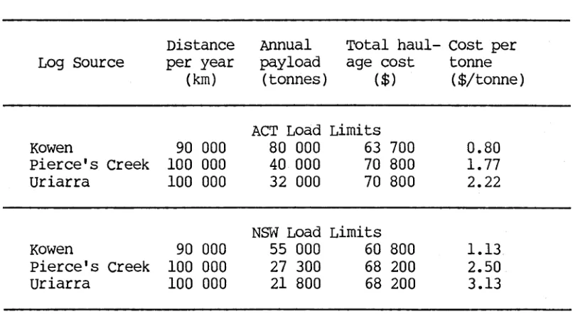
allowed. He compared the cost of log haulage by a typical 5-axle semi-trailer under the 48 tonne gross vehicle weight (gvw) limit imposed by the Forests Branch in the Australian Capital Territory (ACT), with the statutory limit (36.4 tonnes gvw for a 5-axle semi-trailer) imposed at the time in New South Wales (NSW) (Table 1.1). The higher limits for the ACT compared with NSW showed a significant saving in the cost per tonne of hauling woods from these forests; 33 cents per tonne, 73 cents per tonne and 91 cents per tonne for trips from Kowen, Pierce's Creek and Uriarra forests respectively. However a study of loads in Australia and New Zealand showed that some log haulers were not maximizing the load in order to minimize the cost (Ridley 1978). He found wide variations in payloads, "influenced by the attitudes of drivers to fines for overloading and the nature (piece size) of the load carried."

Table 1.1 Costs of log haulage from ACT forests under two load limits

Log Source

Distance

per year

(km)

Annual

payload

(tonnes)

Total haul

age cost

($)

Cost per

tonne

($/tonne)

ACT Load Limits

Kowen

90 000 80 000 63 700 0.80

Pierce's Creek

100 000 40 000 70 800 1.77

Uriarra

100 000 32 000 70 800 2.22

Kowen

90 000

NSW Load 55 000

Limits

60 800 1.13

Pierce's Creek

100 000 27 300 68 200 2.50

Uriarra

100 000 21 800 68 200 3.13

[image:26.533.85.488.469.690.2]

(27)

1.2.3 Speed of Trucks

Matthews (1942) and Shaw (1974) state that the single most important factor affecting the haulage costs for a particular truck is the speed at which the truck operated. However, they noted that a low standard of road only influenced the speed of the truck for that stretch of road, but the payload affected the entire cost of the trip. A study by the New Zealand Logging Industry Research Association (LIRA 1978) concluded that the most significant method to reduce log transport costs was to maximize the distance run per unit time of operation.

1.2.4 Haul Distance

(28)

1.2.5 Delays and Breakdowns to Equipment

Delays and breakdowns also increase transportation costs. Conway (1976) suggests that delays account for up to 20 per cent of the total cycle time and that the actual percentage varies with the haul distance. Smith and Tse (1977) agreed and state that the most serious delays occurred on the landings, either waiting in a queue or waiting for wood to arrive. They suggested a need for improved despatching or better selection of the number of vehicles required.

1.2.6 Managerial Efficiency

The management of log trucks or truck fleets is also a significant parameter in hauling costs. Efficient management of trucks can improve truck utilization and reduce the total hauling costs. LIRA (1979) reported a physical device (Truck Control Board) which accurately and continuously simulates the locations of trucks and simplifies and assists in truck scheduling to reduce delays. McCormack (1983) developed a heuristic allocation algorithm for use in a centralized despatch office and demonstrated that in the operation studied, considerable improvements could be made towards equity in the distribution of work amongst drivers. Determining number of trucks is also important in reducing total hauling costs. Too many trucks may produce long queues at landings and the mill, while too few trucks under-utilize the loaders and increase total costs.

(29)

whole operational system must be examined "as increased productivity alone does not necessarily mean reduced total haul costs." Methods to examine the whole operational system are not however straight-forward. Clearly for example, there is the immediate problem of the definition of the whole operational system. Just as clearly, there will be changes and developments in log haulage systems, with innovations and inventions to equipment and system organisation. These may be seen as part of an operational system. Nonetheless, a rigorous examination of an operational system seems the best basis for insights toward improvements to the system and its management and in turn, lead to cost savings in haulage operations.

1.3 FORMULATION OF THE STUDY

1.3.1 Aims

Haulage costs are becoming increasingly important in Australia as large wood product mills with the necessary economies of scale are constructed in bigger towns but with longer haul distances from wood supply areas and as more small mills close to forests are amalgamated into large efficient mills situated further from individual forests. There is already a great diversity in the log haulage operations to mills and as the scale of individual operations rises, the problems of planning and evaluating the operations in terms of efficiency are becoming more complex.

(30)

determined as the formulation and evaluation of a procedure to assess the efficiency of log haulage systems. In general, the procedure defined and adopted was to:

1. develop a stochastic simulation model, of general application, to assess and improve the operational efficiency of log hauling to a centralized mill

2. undertake a case study and obtain data to develop and statistically validate the model

3. apply the model to the case study to plan optimal log hauling operations and compare the cost of haulage when trucks are leased or purchased.

It was necessary to conceptualise a model of log haulage and this was named the "abstract model".

1.3.2 The Abstract Model

The cycle time of a truck, that is, the interval between two successive departures of a truck from the mill, is as follows:

(1) Cycle time = (travel to landing + load time + travel to mill + unload time + associated delays)

The associated delays represent trucks queueing for resources such as the loaders and unloaders, any breakdown or accidents that delay trucks and deliberate idleness by drivers.

(31)

between trucks, loaders and unloaders cannot be predicted deterministically. If the events in (1) are treated separately, the cycle time can be modelled as in (2):

(2) Cycle time = f(travel to landing) + f(load time) + f(travel to mill) + f(unload time)

where f(-) represents a time selected from the function representing the distribution of the times associated with that component of the cycle.

Associated delays would be incorporated into each of the functions for the events.

Using (2), it is possible to model the trucks travelling between the mill and the landing provided that each function is defined.

Operations Research techniques were examined to select appropriate techniques, to synthesize a working model for a truck fleet with trucks interacting with each other but cycling in accordance with (2).

1.4 OPERATIONS RESEARCH

1.4.1 Introduction

(32)

"had it not been for the digital computer, operations research with its large scale computational problems would not have acquired the present promising status."

(Taha 1982)

A common purpose of an Operations Research program is to improve the effectiveness of the total system defined for study (Daellenbach and George 1978) and methods for evaluation of the response of a system to decisions made by management are an essential requirement. The basis of the evaluation of response in Operations Research is the construction and use of models (Phillips et al 1976).

The application of Operations Research to harvesting systems thus requires the development of a model or models of the system to be studied.

1.4.2 Classification of Models

A model is a simplified representation of an observed process which is used to explain or predict the behaviour of the real world process (Mihram 1971). Models may be classified into 3 groups (Fishman

1973 and Taha 1982): 1. Physical

2. Analogue 3. Symbolic

(33)

Analogue models represent a real system with an analogue which behaves in the same way as the real system, for example, an electrical circuit representing a mechanical or hydraulic system. Analogue models are often used to represent dynamic and continuous processes (Emshoff and Sisson 1970).

Symbolic models, also known as abstract or mathematical models, use mathematical relations to describe the status of variables and the operations and interactions between elements of a real system (Filmer 1978). They use a specific and logical language to represent the system.

Radford (1967) suggests that

"the very act of constructing a mathematical model enforces precision since it requires a specific statement of what is meant."

This is often seen as an advantage of mathematical models for not only must the interrelationships between the variables describing the system be specifically defined, but also the assumptions and constraints.

Symbolic models can be further classified as: 1. Static or dynamic

2. Continuous or discrete

3. Deterministic or stochastic.

Static models either omit time from the model or take a 'snapshot' of the system at one point in time, for a given set of conditions

(34)

with the allocation or design of buildings, where the passage of time has no effect on the system. Dynamic models are concerned with systems which have a variable response with the passage of time.

A continuous model has dependent variables which change in a continuous fashion and the objective in modelling is to observe the continuous variation of dependent and independent variables. A chemical reaction is often represented by a continuous model. Discrete models also involve the passage of time but the variables within the system take discrete values. Furthermore, variables change value at discrete points in time which coincide with events that alter the status of variables within the system.

A deterministic system has variables and interrelationships defined by fixed mathematical or logical relationships and no uncertainty is inherent in the outcome of the system. Thus, for a given input, a deterministic model always produces the same output. A stochastic model has uncertainty implied where part of the variation is random (Fishman 1973). Such models respond with an output associated with a certain probability, and thus a range of outputs can be generated for a given input.

(35)

A range of symbolic or mathematical modelling techniques and procedures has developed under the umbrella of Operations Research and include linear programming, integer programming, dynamic programming, decision theory and heuristics and the numerical techniques of simulation.

Previous studies (Ada 1979) had indicated that a simulation model may be appropriate to analyse log hauling systems and further investigations of simulation modelling techniques were therefore undertaken in relation to the general aims defined for the study.

1.4.3 Simulation

Naylor et al (1966) define simulation as

"a numerical technique for conducting experiments on a digital computer, involving certain types of mathematical and logical relationships necessary to describe the behaviour and structure of a complex real-world system over extended periods of time."

Lehman (1977) sees the theoretical considerations as a main reason for study by simulation, since simulation models are often the "outgrowth of theory" as it becomes impossible to describe a problem with mathematical equations and derive analytical solutions. Hypotheses may be evaluated by the use of simulation models and theories may be re-written with more complexity and understanding after simulation analysis.

(36)

costly or impossible to perform and the development of a simulation model is the only feasible approach to enable experimentation. Morgenthaler (1961) lists eighteen reasons for and benefits from the use of simulation.

One major benefit is that the modeller must view the problem in terms of the total system and this may avoid such problems as suboptimization (Bare 1971, Newnham 1973 and Kleijnan 1974). Another is the compressing or expanding of time, for example a model may simulate in only seconds what are years in the real world system. Thus, there may be replication and development of experiments with the model in only a fraction of the real world time. Simulation models also enable examination of a real world process over very short intervals of simulated time, much shorter than would be possible in the real world

(Fishman 1973).

Naylor et al (1966) suggest that the observation of the real world and the design of the corresponding simulation model may in themselves lead to a better understanding of the system, perhaps proving more valuable than the results of the simulation experiments. Once the model is constructed, it can be used in experiments to analyse different systems as many times as desired and in turn, the output can be used in further analysis. This output can be collected from the model much more cheaply than from the real world (Schmidt and Taylor 1970).

(37)

involves all the statistical complications involved in design and analysis of experiments. Optimization is not inherent within simulation and other Operations Research techniques may be necessary for this purpose.

A major difficulty of simulation is the validation of the model. Validation compares the output from the model with the performance of the real system and is a measure of the reality of the model. However, there are no universally accepted statistical procedures that can be used to validate all system models and validation may rest finally on acceptance by the modeller of the model as a realistic simulator (Van Horn 1971). A simulation model may parallel reality very closely, so that the model becomes as complex as the system being studied. This may be seen as an advantage but it can be a disadvantage if

"the assumptions incorporated in the model are complex and their mutual independence are obscure, (then) the simulation program is no easier to understand than the real process."

(Dutton and Starbuck 1971)

Thus, simulation is not a panacea. It is inherently an abstraction and simulation output only provides estimates of the response variables and the models usually only compare alternative systems rather than generating the optimal alternative.

1.4.4 Methodology of Model Development

(38)

interactions between the variables that comprise the system (Naylor et al 1966, Mize and Cox 1968, Emshoff and Sisson 1970 and Phillips et al 1976):

1. Definition of a problem or problems in an operational system and a statement of the objectives of the study

2. Formulation of a conceptual model 3. Data collection and processing

4. Construction of the computer program to run the model 5. Verification and validation of the model

6. Experimentation and analysis of the results 7. Implementation of the results.

The number of steps and their order is dependent on each particular problem. However, the general sequence of steps is common to all problems (Emshoff and Sisson 1970).

The first step, that is, definition of a problem and a statement of objectives, is of course fundamental. The objectives usually arise from managers seeking improved efficiency. However, the objectives of the study may be stated in only qualitative terms by the managers and the modeller must then translate these into a quantitative basis, known as the objective function.

(39)

"problem formulation is a sequential process that usually calls for continuous and progressive reformulation and refinement of the experimental objectives throughout the duration of the experiment".

(Naylor et al 1966)

1.5 HARVESTING AND TRANSPORT SIMULATION MODELS

1.5.1 Harvesting Simulation Models

Simulation techniques have been successfully applied to harvesting models concerned with the extraction of wood to the roadside, but most of the models have concentrated on the simulation of the harvesting technique. The transport of wood from landing to the mill has not received detailed attention. The following harvesting models included transport from landings and were assessed in relation to their application to this study:

1. Timber Harvesting and Transport Simulator (THATS) (Martin 1975) 2. Auburn Pulpwood Harvesting System Simulator (APHSS) (Goulet et al

1979)

3. Forest Harvesting Simulation Model (FHSM) (Webster 1975)

4. Full-tree Chipping and Transport Simulator (FCTS) (Bradley et al 1976)

5. Harvesting System Simulator (HSS) (O'Hearn et al 1976).

(40)

efficient simulation-oriented languages now available. Finally, many of the models were too restrictive. Some, such as the APHSS model were deterministic in nature and only gave averages as results while THATS advanced time in fixed intervals of one minute, which for the transport phase, was inefficient.

1.5.2 Transport Models

The literature search revealed only two major transport models directly related to the aims of this study. The first was a model simulating the hauling of cane to mills in the sugar cane industry (Sorenson and Gilheany 1970). This model embodies many of the principles of a log hauling simulation model and is reviewed below.

(41)

The other model was developed by the Pulp and Paper Research Institute of Canada (PAPRICAN) (Routhier 1974). The model is based on the GASP (Routhier op.cit.) language and was developed for the analysis of pulpwood and sawlog hauling systems with trucks travelling from one or several loading areas to one mill site. The model simulates breakdowns and repairs for trucks, loaders and unloaders and supplies spare machines to replace those broken down, input data for loading, unloading and haul times are empirical normal distributions. There is no description of the road classification, input data on the duration of breakdowns for machines follows an exponential distribution. The program was tested against a company trucking fleet and found to be a reasonable representation of the system (Routhier op.cit.).

The review of simulation models associated with wood transport showed that most are associated with harvesting systems and that with one exception, the transport phase from the roadside to the mill was not well developed. The exception was the PAPRICAN model. While this model is a dedicated wood transport simulator, it has limitations as a basis for a generalised wood transport model for application to Australian log hauling systems. Only three loading zones are permitted in the model with a maximum of fifteen trucks. It was concluded that it was necessary to develop a new generalised model.

1.6 THE CONCEPTUAL MODEL

1.6.1 Introduction

(42)

the recognition of system variables (Karplus 1977, Osbourne and Watts 1977 and Hillier and Lieberman 1980). These matters are therefore a part of the formulation of the conceptual model of the system which is

"a concise, systematically organised statement of the process, including the specification of the input and the output, the processes and the subprocesses involved, the variables and constants and the data organisation".

(Lehman 1977)

The model can be specified as dynamic or static, continuous or discrete and deterministic or stochastic. The constraints imposed by costs, nature of the system and technology help determine both the system variables and interactions that may be modelled. These, in relation to the objectives of the model, will indicate the appropriate level of detail adopted to simulate reality.

In formulating the conceptual model, it is essential for the modeller to be familiar with the system to be studied. The modeller then knows how it works and is better able to define the variables, parameters and the underlying theory of their behaviour. Emshoff and Sisson (1970) suggest approaches to identify the critical variables in an unfamiliar system:

1. the flow approach

2. the functional approach 3. the state-change approach.

(43)

into the sequence in which they occur. The state-change approach identifies processes which change the state of the system and the times at which they occur.

"Variables" are quantifiable properties of the system that take on different values during the simulation while "parameters" are "quantifiable properties that control the behaviour of the system variables according to the functional relationships which specify the behaviour of the model" (Osbourne and Watts 1977). Parameters have only one value during a simulation run, but can be changed between runs.

The variables and parameters of a system can be classified as exogenous or endogenous. "Exogenous" parameters and variables are the specified inputs of the model and are independent of the model. They can be classed as controllable or noncontrollable. The former can be modified by management and the latter are generated by the environment of the model system. "Endogenous" parameters and variables are the output of the simulation model with their values determined by the interactions within the model.

However, an element of a system may be classified as a parameter or variable, exogenous or endogenous, controllable or noncontrollable, depending on what part of the system is studied, the level of detail required and the objective of the simulation model.

1.6.2 The Dynamics of Log Haulage Systems

(44)

responses of the system to decisions on the operation of the system. Therefore, a simulation model for the study of such a system must be both dynamic and stochastic.

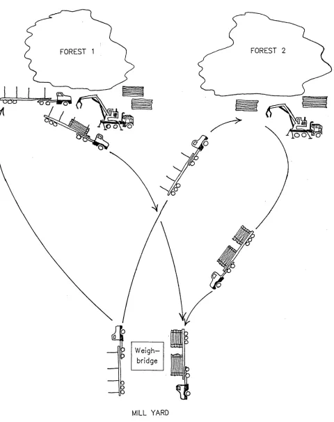
The state-change approach suggested by Emshoff and Sisson (1970) can be used to identify the relationships, variables and parameters of consequence in a log hauling system. These are shown in Figure 1.1. The status of the system changes only at discrete points. For each truck, these are when a truck arrives at the landing, when it starts loading, when it leaves the landing, when it arrives at the mill, and so on. The predicted wood flow from the landing to the mill is thus a result of the sequential processes among the trucks, loaders and unloaders.

Thus, the state-change approach enables identification of processes at the landing and the mill which change the state of the system. Since these changes occur at discrete times, an appropriate method of simulation would be to use a dynamic, stochastic, discrete event-oriented model.

(45)

Figure 1.1 Schematic diagram of a generalised hauling system

FOREST 2 FOREST 1

■oner

Weigh—

[image:45.533.25.505.124.730.2]

(46)

Table 1.2 Quantifiable properties of the truck fleet in a generalised hauling system

ITEM Exogenous non

controllable parameter

Exogenous controllable parameter

Endogenous variable

Number of trucks X

Type of truck/trailer combination

X

Maximum hours allowed to work per day per shift

X

•

Haul times to and from forests

X

Loadweights carried X

Load time of trucks X

Start times of trucks in morning

X

Hours worked by trucks X

Cost of trucking operation

(47)

to start earlier or later. The model produces two endogenous variables, the hours worked by the trucks and the resulting cost of the trucking operation. The quantifiable properties for the loaders and mill are detailed in Table 1.3

The above variables, parameters and processes constituted the conceptual model of a log hauling operation to a centralised mill. The following exogenous noncontrollable parameters would vary in an actual hauling operation and in relation to a conceptual model, were envisaged as random events selected from a frequency distribution of times for that parameter:

1. Haul times to and from forests 2. Load times of trucks

3. Unload or time spent in the mill by trucks 4. Loadweights carried by trucks.

The sequential processes and the frequency distributions for the exogenous noncontrollable parameters are illustrated in Figure 1.2 and are the basis of the conceptual model.

1.7 THE CASE STUDY

1.7.1 introduction

(48)

Table 1.3 Quantifiable properties for loaders and unloaders in a generalised hauling system

ITEM Exogenous non Exogenous Endogenous controllable controllable variables parameters parameters

Number of loaders

x

Time of unloading X

Scheduled hours of work

x

for loader

Start times in morning

x

Opening and closing time

x

of weighbridge X

Hours worked by loader X

Cost of loading operation X

Number of loads and tons X

(49)

[image:49.533.40.507.74.781.2]

Figure 1.2 Sequential processes and exogenous noncontrollable parameters of the conceptual model

Number o f tr u c k s

Number o f loaders

Loader hours FOREST

Weighbridge or m il l hours

LOADER

FIFO QUEUE

Load tim e Loadweight

Travel to m ill

Travel to landing

QUEUE Weigh—

FIFO QUEUE

Mill Yard

Time in m ill

(50)

improvements to an existing system could be evaluated, real rather than synthetic data could be used and the magnitude of the effort in obtaining the real data could be assessed.

Australian Newsprint Mills Ltd. (ANM) were in the process of completing a large centralised pulp and paper mill at Albury, (New South Wales (NSW) at the time this study was initiated. There were several

advantages in using this operation as a case study:

1. It was relatively close to the Australian National University

2. Long haul distances were involved, with up to 200 kilometres one way

3. Several loaders and a relatively large (for Australia) truck fleet were required.

ANM agreed to provide access to their records.

1.7.2 The ANM Operations at Albury, New South Wales

1.7.2.1 The overall system

At maximum annual production, the mill requires 477 000 tonnes of plantation grown softwood to produce 180 000 tonnes of newsprint. The geography of the operations is shown on Map 1.1.

(51)

Map 1.1 The area of supply for the ANM mill

T umut

" --- ^ X

)

Bat low

Holbrook

T umbarumba

Albury

Shel ley

Myrtleford

Softwood plantations

15 30 4,5 Kilometres

Highway

Scale

(52)

mill also imports a small amount of long-fibred semi-bleached Kraft pulp.

The NSW area of supply encompasses five main forests: Bondo, Batlow-Bago, Green Hills, Mannus and Carabost. The average one way haul distance is 206 kilometres. The Victorian area of supply encompasses the forests of Koetong-Shelley, Beechworth, Myrtleford and Bright for which the average one way haul distance is 111 kilometres.

The majority of timber comes from either first or delayed first thinnings. In some operations, both pulp and sawlogs are produced and the logs are sorted within the forest for different destinations. ANM harvests the wood with a mechanical harvesting system. The Kockums Logma system produces timber between 3.6 and 5.4 metres in length. The control of the wood procurement operation is separated into harvesting,

loading and transport operations.

The following brief description of the operations provides a background to the formulation of the study.

1.7.2.2 The harvesting system

ANM employs ten harvesting contractors, each using the Kockums Logma System. The system comprises an 880 feller buncher, an 85-41 Logma processor and an 85-33 forest tractor.