Design and field trial measurement results for a portable and low cost VHF / UHF channel sounder platform for IoT propagation research

Article:

Ball, E. orcid.org/0000-0002-6283-5949 (2019) Design and field trial measurement results

for a portable and low cost VHF / UHF channel sounder platform for IoT propagation

research. IET Microwaves, Antennas & Propagation. ISSN 1751-8725

https://doi.org/10.1049/iet-map.2018.5827

This paper is a postprint of a paper submitted to and accepted for publication in IET

Microwaves, Antennas and Propagation and is subject to Institution of Engineering and

Technology Copyright. The copy of record is available at the IET Digital Library.

Reuse

Items deposited in White Rose Research Online are protected by copyright, with all rights reserved unless

indicated otherwise. They may be downloaded and/or printed for private study, or other acts as permitted by

national copyright laws. The publisher or other rights holders may allow further reproduction and re-use of

the full text version. This is indicated by the licence information on the White Rose Research Online record

for the item.

Takedown

If you consider content in White Rose Research Online to be in breach of UK law, please notify us by

Submission Template for IET Research Journal Papers

Design and field trial measurement results for a portable and low cost VHF / UHF

channel sounder platform for IoT propagation research

E. A. Ball

1 _{Department of Electronic and Electrical Engineering, The University of Sheffield, Sheffield, S1 4ET, UK}

e.a.ball@sheffield.ac.uk

Abstract:Propagation research is vital for informing the design of reliable VHF and UHF communications systems for the Internet of Things (IoT). In this paper, a cost-effective and highly portable system is proposed and then used to obtain propagation measurements in city and suburban scenarios at 71 MHz and 869.525 MHz. The system calculates the received power, power delay profile and channel frequency response. The portable sounding receiver uses readily available parts: an RTL-SDR (covering 27 MHz 1.7 GHz) and a Raspberry Pi with touchscreen. The Pi implements all the channel sounding

signal processing algorithms in Python, in near real-time. Extracted propagation data and models are presented, from example city and suburban field trials incorporating pedestrian and car use.

1. Introduction

Industrial and commercial interest and application of the Internet of Things (IoT) continues to grow, with both standards-based solutions and multiple proprietary systems jockeying for adoption. Emerging systems include NB-IoT and also 802.11ah “HaLow” [1] as well as the commercial LoRa [2] and Sigfox [3] systems. Even though systems are being brought to market, there still exist many fundamental research opportunities for antennas and propagation, in IoT specific use cases. There is also a need for practical systems to evaluate propagation performance and link budgets, for commercial applications and also for use in student teaching. A particular area of valuable research involves long range RF systems that are very low power and low cost, possibly powered by coin cells (e.g. CR2032) and supporting high reliability use cases, with multi-year life expectancy. Such devices could serve, for example, in connecting future city infrastructure or ubiquitous social care and healthcare systems.

VHF spectrum at 55-68 MHz, 70.5-71.5 MHz and 80.0-81.5 MHz has been promoted by Ofcom in the UK for use in IoT applications [4]. In the EU, Short Range Devices (SRD) spectrum in 863-870 MHz is widely employed for generic radio systems [5] and is where many commercial EU IoT systems currently operate. This is comparable to the 915 MHz Industrial Scientific & Medical spectrum widely used in the USA and Oceania.

Future high reliability and novel IoT radio systems may exploit multiple RF bands as well as reconfigurable modulation and cognitive radio aspects. This all requires fundamental, real world, understanding of the radio spectrum occupancy and usage, as well as propagation and noise floor characteristics for the bands.

To assist in the capture of IoT VHF and UHF propagation information, a low-cost, portable and frequency-agile system has been created and is described in this paper. The system consists of a fixed transmitter and a pedestrian portable Channel Sounding Receiver (CSR) [6]. The CSR allows near real-time capture and display of the channel

response in operational environments, such as urban canyons or remote rural locations. The CSR system is built using an RTL-SDR and Raspberry Pi 3B (R-Pi) with touchscreen- all powered by a USB battery power pack. The RTL-SDR imposes a maximum RF capture bandwidth (BW) of 2 MHz, but this is considered sufficient for our IoT propagation measurements since IoT radio systems for long range tend to not use multi-megahertz RF BWs (often significantly less).

This paper continues in section 2 with a discussion of IoT propagation; the channel sounding hardware used in section 3; channel sounding algorithm design in section 4 and lab testing of the system in section 5. Section 6 presents example measurements from a small scale city field trial campaign, followed in section 7 with results from a suburban measurement campaign. Section 8 presents models for the extracted propagation path loss data, suitable for use in IoT link budgets. Section 9 presents values for RMS delay spread, estimated from the field trial results.

The contributions of this paper are: 1) creation of a novel, low-cost, portable, near real-time channel sounding platform, 2) development of efficient algorithms for extracting the channel power delay profile and frequency response, 3) usage of the system to obtain example propagation data in suburban and city environments; leading to simple propagation models for use in IoT system design.

2 devising and creating novel future IoT systems, which may

address un-met use cases. The VHF and UHF spectrum is particularly attractive for long range communications, though antenna efficiency is often challenging. VHF and UHF propagation has been extensively studied over the years, for both commercial and military uses (e.g. [8], [9], [10]). There have also been investigations into short range applications [11].

Previously reported VHF and UHF RMS delay spreads have been observed to be typically in ranges of 100 ns to 2 µs at distances of up to 2 km in various urban settings [12], [13], [14], [15] though occasionally reaching 5 µs when indoor-outdoor transitions are included [16]. In contrast, the delay spreads in mountainous regions at VHF have achieved 8 µs [13] to 30 µs [17]. Propagation from devices with antennas near to ground, using VHF spectrum, has been shown to include significant path loss effects due to building roof line knife-edge diffraction [18].

Traditional path loss models focus on broadcast or cellular systems so are not relevant or representative of the use cases for IoT. New research is now developing propagation models for VHF systems that are close to ground for short range outdoor applications [19], [7], [15] and indoor-outdoor transitions [20], but the need for a compact and portable low cost CSR is clear, to provoke and enable further research.

Short range communications research has shown that multipath effects are less significant at VHF [19], [20] due to the reduced size of scatterers compared to the wavelength, manifesting itself as propagation with low delay spread.

In a general RF communications system it is highly desirable to use a symbol duration significantly longer than the RMS delay spread, since channel equalisation can be avoided. Such possible reductions of complexity are vital to cost-effective IoT applications. Since reported RMS delay spreads are typically less than 2 µs therefore implies a 20 µs minimum symbol duration would be desirable.

The CSR system proposed in this paper can be used to investigate and characterise propagation delay spread and channel conditions for any use case in the field and, although currently focused on 869 MHz and 71 MHz bands, could be deployed to measure anywhere within the frequency range of the RTL-SDR and companion transmitter or signal generator.

3. Channel Sounding Receiver Hardware

The channel sounding system consists of a transmitter and receiver. The transmitter is either an RF vector signal generator or a dedicated companion channel sounding transmitter (both are operated at a fixed location). The Channel Sounding Receiver (CSR) is highly portable and incorporates a display for channel impulse Power Delay Profile (PDP) and frequency response. In the tests presented here an Agilent E4437B signal generator is used as the TX signal source, loaded with waveform files created to suit the CSR. A dedicated companion transmitter has also been created and demonstrated at 71 MHz, which is the subject of future papers. The hardware used to make the CSR consists of:-

• Raspberry Pi 3B

• Raspberry Pi 7” or 3.5” touchscreen & case • NooElec RTL-SDR with 0.5 ppm reference oscillator

• 5.4 Ahr portable USB battery pack

Fig. 1. RTL-SDR & 7” Touchscreen CSR, showing example 869 MHz channel PDP and frequency response.

Fig. 2. RTL-SDR & 3.5” Touchscreen CSR, 869 MHz

antenna attached.

The complete cost for the 3.5” touchscreen CSR variant is circa £85, making it extremely cost-effective for both research in VHF / UHF propagation and teaching applications. Both CSRs are shown in operation in Figs. 1 and 2. The use of a USB extension lead is important since it allows the RTL-SDR and its associated antenna to be placed optimally for the propagation trial and also helps separate it from sources of RF interference in the R-Pi. Ferrite clamps on both the USB cable and RG316 coax were also found to be essential: further reducing interference from the R-Pi that can otherwise desensitise the RTL-SDR, particularly at 71 MHz.

4. Channel Sounding Algorithm

The transmitting signal generator is used to illuminate the channel with a known BPSK modulated Pseudo Random Binary Sequence (PRBS). The same PRBS sequence is used in the CSR to perform a correlation against the received signal and thus extract the channel response. The CSR performs all the Digital Signal Processing (DSP) on the captured IQ data

waveforms using Python and is able to display the extracted time domain and frequency domain plots to the user in near real time (under 5 seconds).

4.1 PRBS M-Sequence Selection

3 sounding activity, which avoids the need for any spreading

code acquisition stages prior to sounding and thus reducing complexity. It is also beneficial to avoid the need for any frequency acquisition stage after data capture; further reducing complexity. Although the R-Pi is a capable platform for code development and execution, the avoidance of the above stages helps minimise the processing time in the field. The need for carrier frequency acquisition can be avoided by recognising that if the phase rotation of the RX IQ data (due to frequency errors) is less than 180 degrees over one complete PRBS frame then BPSK signals can be demodulated without error. The limiting relationship between maximum PRBS frame length and overall frequency error (composite of RX oscillator error and TX carrier error) is shown in (1).

(1)

In (1),

is the duration (seconds) of a single PRBS frame

Intermediate Frequency (IF). The worst-case frequency errors are 0.5 ppm for the RTL-SDR and 1 ppm for the ESG4437B TX signal generator. The RTL-SDR is capable of sampling IQ data at 2 Msample/s, which would provide a direct conversion captured RF BW at the carrier of 2 MHz. To obtain the maximum channel temporal detail requires maximum illuminated BW, so a BPSK bitrate of 1 Mb/s was chosen, thus occupying the 2 MHz IF BW to the first sinc nulls. Clocking the PRBS symbols at 1 Mb/s and applying (1) predicts the CSR should tolerate IF frequency errors of up to 978 Hz. To achieve this long term would require GPS-lock of the TX signal generator and CSR, which is inconvenient. The RTL-SDR uses an internal temperature compensated crystal oscillator and the ESG4437B has a temperature controlled oven, so perceived carrier drift is minimal in practice, which allows the considerable simplification of applying an experimentally determined carrier offset correction to the TX signal. This ensures that the overall error at the CSR IF is manually controlled to below 978 Hz. The ESG4437B internal reference has proven to be very stable after warming up, hence this initial correction approach has proven acceptable for the duration of all measurement campaigns so far.

4.2 Correlation Technique in Channel Sounding Receiver

The CSR’s main task is to perform a correlation between the received IQ data and the known TX PRBS sequence. This correlation can be performed in the time domain, but this is not computationally efficient. A more computationally efficient alternative is to perform the correlation of the two signals via the frequency domain [21], [22], [23] using convolution and then return the result back to the time domain. It is this Fast Fourier Transform circular convolution (matched filter) approach that is employed in the CSR, described in (2).

In (2), H(f) and G(f) are the Fourier transforms of time series h(n) and g(n) respectively and * denotes complex conjugation.

C is the resulting cross-correlation array of the time series, resulting from the Inverse Fast Fourier Transform (IFFT) operation. Python code in the R-Pi interfaces to the RTL-SDR as well as implementing the required DSP algorithms and thus providing near real-time visualisation of the delay spread and frequency response of the propagation channel at a particular location. The CSR algorithm was written in Matlab and Python, allowing students to follow and modify the code. The RTL-SDR’s internal RX gain is set to 49 dB and configured to capture samples representing 32 full PRBS frames, storing the captured data to file for analysis. The CSR algorithm to be described is based on a simplified version of those used in [21], [22], [23].

In the following descriptions, variables holding arrays of samples are italicised and in bold. Assume there are N complex samples per received PRBS frame (PRBS sequence length 511, oversampled by factor 2, i.e. N = 1022). The RX data from the RTL-SDR is partitioned into segments of length 2N: rx_sequence_2N[1..2N], which facilitates robust detection of at least one strong correlation peak, regardless of time offset in the captured RX data, compared to the TX PRBS. The overall captured RX data file is then processed in 16 such segments, each of length 2N samples, using the following pseudo-algorithm [6]:

1. Since the FFT input data must be periodic in time and the RX data is processed in lengths of 2N, the TX correlation sequence of length N (for matched filtering) must be extended with zeros to length 2N:

tx_sequence = concatenate [PRBS, zeros(N)]

2. Compute the FFT of the time domain TX sequence:

T = FFT(tx_sequence). This can be calculated in

advance since it is fixed.

3. Select segment K in turn (0..15) of length 2N samples from the captured RX data rx_data:

rx_sequence_2N = rx_data[K2N : (K+ 1)2N-1]

4. Compute the FFT of Kth time domain RX segment:

R = FFT(rx_sequence_2N)

5. Compute the conjugate of the frequency domain representation of received data:

Rconj = conjugate(R)

6. Compute the delay profile for segment K by element-wise multiplying Rconj & T and then taking inverse FFT: time_response = IFFT(Rconj

.

7. Finally, compute the delay profile magnitude of segment K: time_response_mag =

abs(time_response)

4 responses can then be summed to produce a composite

channel frequency response for the CSR’s location. The sinc response of the BPSK signal is imposed on the RX channel spectrum, requiring steps be taken to equalise it. The RTL-SDR was also found to add further non-linearity as a function of RX signal level. Thus, amplitude equalisation was required to address both issues. The BPSK frequency domain response, for use in equalisation (after inversion), at FFT bin x out of N is given by (3).

(3)

From lab characterisation of the RTL-SDR, exponent n is selected based on the magnitude of the maximum time domain RX signal correlation peak, Cp, using (4a) or (4b).

ln

(if Cp< 4500) (4a)

(if Cp> 4500) (4b)

Cp is the maximum value seen in time_response_mag array and also directly represents the RX RF power at the test location. The conversion of the correlation peak value Cp to an equivalent RF RX power is performed using (5).

log dBm (5)

The conversion offset value of -159.8 dBm in (5) was found experimentally during lab calibration and represents the composite gains of the RTL-SDR hardware and cable losses.

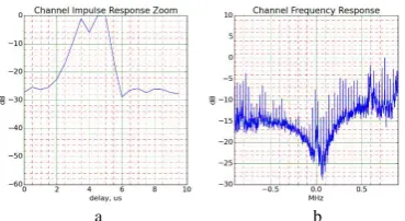
5. Testing of the Channel Sounding System Prior to field use of the sounding system, it was subject to performance testing and calibration. Tests using a simulation model of a reflective channel were performed first, to validate the CSR algorithms. The simulated channel consisted of a primary ray with 1 reflection of delay 53 µs and with the same amplitude. The correctly extracted impulse response is presented in Fig. 3a with a primary signal visible at 100 µs offset and 1 reflection with path delta of 53 µs. Fig. 3b shows the corresponding frequency response of the simulated channel. A 53 µs delay in the channel model should present itself as spectral peaks and nulls with a period of 18.9 kHz and this matches well with Fig. 3b.

The ability of the CSR to resolve emulated reflections was also tested. Here, the ESG4437B produced the CSR’s PRBS modulated BPSK signal and the signal from a separate (unsynchronised) VHF channel sounding transmitter were attenuated and then combined - representing a primary path with 1 random reflection delay. The CSR was then used to extract the impulse response from the resulting composite signal. Since the signal generator and TX sounder were not synchronised, the time separation between impulses is random for each test. Fig. 4 shows the CSR captured impulse response for the 2 equal amplitude signals, resolved at 53 µs apart. With the two signals at the same level, significant spectral nulling occurs, as would be expected. The nulls are visible in Fig. 4b, with 18.5 kHz spacing, which agrees well with the expected 18.9 kHz due to a reflection delay of 53 µs and also with the results of Fig 3.

a b

Fig. 3. Channel response with 1 simulated reflection at 53µs

delay, from a 100 µs primary signal.

(a) PDP, (b) Frequency response with 18.6 kHz null spacing

a b

Fig. 4. Channel response for cabled emulation system, both

signals at -95 dBm.

(a) PDP, (b) Frequency response with 18.5 kHz null spacing

a b

Fig. 5. Channel response for emulation system: signal

generator at -105 dBm & sounder TX at -95 dBm.

(a) PDP, (b) Close up of frequency response

a b

Fig. 6. Channel response for emulation system: signal

generator at -115 dBm & sounder TX at -95 dBm.

(a) PDP, (b) Frequency response

5 Fig. 5b shows circa 6 dB of ripple. As a final reflection

emulation test, the emulated path amplitude difference was increased to 20 dB, resulting in the impulse response shown in Fig. 6. The resulting channel response has circa 3 dB of passband ripple and the spectral nulls are now 15.5 kHz apart, which agrees well with the expected 15.4 kHz due to the 65 µs reflection delay.

Overall, the above results show that the CSR system is working as expected. Note that in all time domain PDP figures, the absolute time delay of the primary correlation peak is random, due to the random initial M-sequence alignments between the TX and CSR RX. The CSR RX power measuring accuracy was tested with conducted signals, prior to use in the field. Table 1 presents the results of the CSR calculating the RX power, using (5).

Table 1 CSR RX Power Test

Conducted RF RX power at 71 or 869 MHz

(dBm)

CSR detected power at 71 MHz (dBm)

CSR detected power at 869 MHz (dBm)

-80 -75 -76

-90 -87 -87

-100 -99 -100

-110 -109 -110

-120 -121 -122

-130 -131 -131

When a conducted signal without a reflections is received, the CSR is expected to produce a flat channel response and single correlation peak. This is confirmed for both bands in Figs. 7 and 8, using a test signal of -90dBm.

a b

Fig. 7. 71 MHz Conducted channel response (-90dBm). (a) PDP, (b) Frequency response

a b

Fig. 8. 869 MHz Conducted channel response (-90dBm). (a) PDP, (b) Frequency response

The lab measured conducted sensitivity of the CSR is -125 dBm at 71 MHz and -130 dBm at 869.525 MHz, both for a displayed 10 dB correlation peak to noise ratio.

6. City Field Trials

One of the main purposes of the CSR is to facilitate rapid measurements of channel response and path loss in portable and mobile use cases. The frequencies investigated were centred on 71 MHz and 869.525 MHz, representing the two IoT bands of interest. To support pedestrian portable field tests, a commercial 868 MHz sleeved dipole whip antenna and a custom 71 MHz loop antenna were used, as shown in Fig. 9. For each case, the CSR test antenna was held at arm’s length and with the radiating structure approximately at the operator’s head height.

Initial field trials of the CSR in a pedestrian mobile test route through Sheffield city centre (53°22’50”N, 1°28’40”W) produced early results, select examples of which are reported in this section. The TX modulated source was the ESG4437B signal generator feeding a VHF folded dipole, or UHF whip, as appropriate, both mounted on a first floor office window.

The bespoke 71 MHz loop antenna had a BW of circa 200 kHz, which superimposed its response onto the extracted propagation channel response. The imposed BW limit can be seen, for example, on Fig. 10b. (This unwanted frequency response could be modelled and equalised from the CSR results, if required.)

Fig. 9. Portable RX test antennas for 869 MHz (whip on left)

and 71 MHz (loop on right).

a b

6 a b

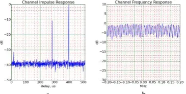
Fig. 11. 71 MHz Channel impulse response (190 m). (a) PDP, (b) Frequency response

Fig. 10 show an example channel impulse PDP and frequency response for measurements at 71 MHz with the CSR circa 76 m from the TX source. Fig. 11 show channel delay and frequency response for measurements at a non-line-of-sight street location circa 190 m from the sounder TX. Note the in-band tone interference on the extracted channel frequency response of Fig 11b.

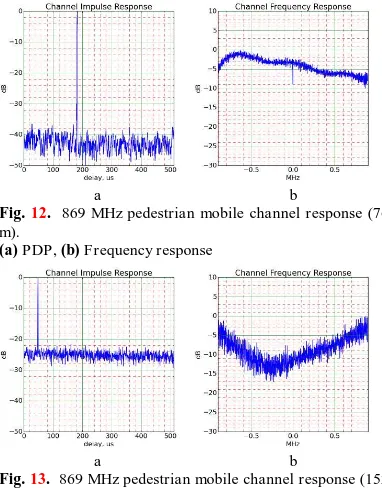
Measurements were then taken on the same pedestrian mobile route incorporating the same test locations, using 869.525 MHz. The UHF test antenna used was broad band, so gave negligible shaping to the recovered spectrum. Fig. 12

shows an example channel responses extracted for a measurement location. The slope of the channel frequency responses suggests a sub 1 µs delay spread, which is plausible since no echo signal was seen resolved in the time domain. Delay spread calculations based on all observed PDPs are presented in section 9.

a b

Fig. 12. 869 MHz pedestrian mobile channel response (76

m).

(a) PDP, (b) Frequency response

a b

Fig. 13. 869 MHz pedestrian mobile channel response (152

m).

(a) PDP, (b) Frequency response

a b

Fig. 14. Example interference observed in 71 MHz city tests. (a) MS2712E time domain (zero span), (b) Close up of

resulting frequency response from CSR

Fig. 13 shows a single broad null, again suggesting a delay spread of significantly less than a 1 µs. As before, no echo is seen with delay exceeding 1 µs. Most of the measurements made during this test route showed a broadly flat channel response.

Although the delay spreads in the 71 MHz and 869 MHz examples are expected to be low (due to short distances), interesting channel frequency responses are still observed, which can inform use case link budget design. Extracted channel path loss models using the data are presented in section 8.

During the city tests, several locations were noted where interference was present (usually seen on the channel frequency response). During a subsequent investigation using a portable spectrum analyser (Anritsu Spectrum Master MS2712E) and antennas, the presence of sources of RF interference at various CSR field test locations was confirmed; with observed RX powers up to -100 dBm at 869.5 MHz and -80 dBm at 71 MHz (measured in a 10 kHz BW). The interference was often elaborate and intermittent, presenting as both an increase in white noise as well as additional random periodic events. A time domain example from a site with only periodic noise is shown in Fig 14a, as captured on the MS2712E and showing a periodicity of 40 µs. The equivalent channel response recovered by the CSR is shown in Fig 14b, displaying a frequency domain periodicity due to the same interference of circa 25 kHz, as would expected given the time domain signal. The sources of the interference could include commercial and domestic IT and lighting [24] systems as well as other legitimate users of the bands, such as EN 300 220 SRDs.

7 cascaded antenna gains and system conversions are close to

expectations and CSR system operation is acceptable. The 71 MHz loop antenna is directional (maximum gain in the plane of the loop), so select propagation measurements have been performed taking measurements with both 90 degree orientations at each location.

7. Suburban Residential Field Trials

Measurements were also performed around a hilly residential area of Sheffield (53°21’50”N, 1°29’35”W) incorporating mixed housing, trees and vegetation. Two different measurement runs were executed: pedestrian mobile and car mobile. In both cases, the TX antennas were sited 4.3 m above ground at the rear of a dwelling, providing good RF illumination towards both the city and residential areas in the east of the city.

For tests at 71 MHz, a vertically polarised dipole antenna was mounted outside of the dwelling hosting the TX, as shown in Fig. 15. During UHF soundings, the VHF dipole was removed and replaced with a UHF sleeved dipole whip antenna.

7.1 Pedestrian mobile

The pedestrian mobile test route incorporated a journey around the streets near the dwelling. This use case could represent a user installed IoT system, with coverage required around the immediate neighbourhood. The figures presented in this section represent some of the notable channel responses obtained, rather than an exhaustive collection. The actual BW of the 71 MHz RX loop antenna is circa 200 kHz and superimposes its response on the measured channel response, as discussed in section 6.

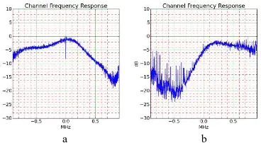
In general, after accounting for the loop antenna’s response, the propagation channel frequency response for the 71 MHz pedestrian mobile scenario was flat - but with some exceptions which are now presented in Figs. 16-17. The deep null on the right of Fig. 16a and on the left of Fig. 16b are in contrast with boosted signal on the other side of their respective plots (compared to the example reference response seen in Fig. 10). This suggests both constructive and destructive signal combination is occurring within the observed frequency range, but with a delay spread that is much less than 1 µs. Fig. 17 shows a deep central null (nulling out the 71 MHz loop antenna’s peak), also with interference. Only one CSR test location provided an observable PDP reflection (value -20 dB). The spectrum for this location was flat, as would be expected for such a weak reflection.

Fig. 15. VHF TX antenna located at the first floor window of

dwelling.

a b

Fig. 16. 71 MHz pedestrian mobile channel response. (a) 198m (b) 314m, with interference

Fig. 17. 71 MHz pedestrian mobile channel response (414

m), with interference.

Fig. 18. 869 MHz pedestrian mobile channel response (107

m).

Measurements were also taken at 869.525 MHz on the same pedestrian test route. Fig. 18 shows a pronounced fade near the band centre and what could be the start of second nulls at +/- 1 MHz. However, at 869.525 MHz the fading was generally flat across the observed spectrum, though sometimes with shallow fades of depth 5dB.

Measurements were made for direct path distances of up to 500 m - with very few observable time domain reflections exceeding the 1 µs resolution, and those that were present always being below -20 dB. This also manifests itself with only a small number of locations presenting with spectral nulls: operation at 71 MHz being more susceptible to such nulls.

7.2 Car mobile

8 IoT system is required to have coverage around a city region.

The CSR RX antennas for 869.525 MHz and 71 MHz were quarter wavelength whips with magnetic mounts in the centre of the car roof. The test route included various elevations with respect to the TX site (differential heights ranging from +83 m to -50 m).

Figs. 19-20 show notable channel responses obtained at 71 MHz during the car test route. Fig. 19b shows the recovered 71 MHz frequency response is notably flatter, due to the use of a broad band UHF whip antenna, rather than the loop. Figs. 19-20 are typical of the VHF PDP and frequency responses in showing broadly flat spectrum and no resolvable reflections, to a 4 km range.

A small number of CSR test locations did present non-flat channel frequency responses, such as Fig. 21. As with previous measurements, the dimensions of the null suggest a sub-microsecond echo delay.

The same car route was then investigated at 869.525 MHz. The majority of spectra collected were either broadly flat or showing only modest shaping due to reflections. For example, Fig. 22 shows circa 5 dB of spectral slope across the measured band whereas Fig. 23 has a slight null of depth less than 5 dB.

There were some distant CSR RX locations providing very good signal levels yet still showing no significant reflections, for example Fig. 24. As also seen in previous tests, some locations did appear to suffer interference, occasionally presenting as tones.

a b

Fig. 19. 71 MHz car mobile channel response (2.87 km). (a) PDP, (b) Frequency response

a b

Fig. 20. 71 MHz car mobile PDP.

(a) 4.05 km, (b) 4.5 km (limit of CSR sensitivity)

a b

Fig. 21. 71 MHz car mobile channel response (418m). (a) PDP, with reflection at -25 dB (b) Frequency response

a b

Fig. 22. 869 MHz car mobile channel response (107 m). (a) PDP, (b) Frequency response

a b

Fig. 23. 869 MHz car mobile channel response (2.71 km). (a) PDP, (b) Frequency response

a b

Fig. 24. 869 MHz car mobile channel response (2.87 km). (a) PDP, (b) Frequency response

9 CSR at longer ranges. However, the paucity of reflections

over all distances is valuable information, possibly supporting the proposal of over-roof knife edge diffraction [18] being a key mechanism.

8. Extracted Propagation Models

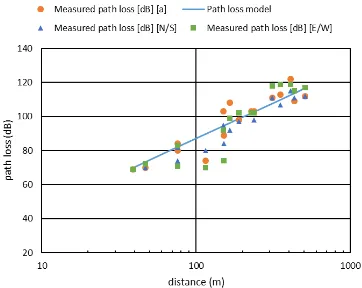
Data was captured from several measurement journeys on each route (1 in summer and 2 in autumn). In addition to the PDP and channel frequency responses, received signal power is also calculated by the CSR, at all the field trial locations. The raw path loss data and proposed straight line approximations are shown in Figs 25-30. Hata small city and suburban path loss models [10] are also included for reference, where applicable. (Note that the lower valid frequency for the Hata model is 150 MHz, so is included only for information on 71MHz figures). The straight line models are all fitted using a least squares approach.

The circled data points on Figs. 29-30 identify locations with a clear Line of Sight (LoS) path to the TX site, which are thus presenting low path loss, compared to adjacent locations. The general observed scattering of the data points is to be expected given the nature of the testing: signal paths partially occluded by various buildings, vegetation and trees, RX antennas at head height and with general movement of vehicles and people in the vicinity of the tests. Furthermore, relatively small changes in the CSR’s location can open up different propagation paths. Additionally, for suburban car tests, locations had to be selected where it was safe to stop.

The data was measured at the same locations (within circa 2m) on 3 occasions: identified on Figs. 26-27 and Figs.

29-30 as [a] in summer, [b] and [c] in autumn. The suburban car based measurements show little variation due to the measurement runs. Autumn pedestrian tests using the 71MHz loop antenna were repeated for loop orientations of North/South (marked [N/S]) and East/West (marked [E/W]) to capture directionality effects on Fig. 25 and Fig. 28. The 869MHz suburban pedestrian tests appear to show a decrease in path loss in autumn; most likely due to the reduced foliage on the test route.

The log-normal (straight line) path loss P model described by (6) is used to fit the measured data to the test scenario distance d; with model-specific coefficients u and n as presented in Table 2.

log dB (6)

Path loss results reported in [19] at 64 MHz measured at 300 m showed losses of circa 97 dB over open flat concrete, 97-108 dB over grass and 100-108 dB for wooded areas. Comparable 71 MHz results presented in this paper show a loss of 96 dB for the suburban pedestrian (and 107 dB for the city scenario) at 300 m.

Fig. 25. City pedestrian 71 MHz path loss data and model.

Fig. 26. City pedestrian 869 MHz path loss data and model.

Fig. 27. Suburban pedestrian 869 MHz path loss data and

10

Fig. 28. Suburban pedestrian 71 MHz path loss data.

Fig. 29. Suburban car 869 MHz path loss data and model

(distant locations with LoS to TX are marked by the circle).

Fig. 30. Suburban car 71 MHz path loss data and model

(distant locations with LoS to TX are marked by the circle).

Table 2 Path loss model coefficients

Propagation scenario n u (dB)

City Pedestrian 869 41 18 City Pedestrian 71 42 3 Suburban Pedestrian 869 42 16 Suburban Pedestrian 71 38 2

Suburban Car 869 26 48

Suburban Car 71 25 20

The Hata small city model at 869 MHz shows good agreement to the fitted model for car mobile data in Fig. 29

(but a 10 dB underestimation in the Hata suburban model). Although the Hata model is not valid below 150 MHz, it is interesting to compare its prediction for the 71 MHz propagation results in Fig. 30 and again it shows good agreement with the small city model at 1km, but is better represented by the Hata suburban model by 5km.

Considering a theoretical, frequency-dependent fixed-loss FL as defined in (7) gives a fixed-loss for 869.525 MHz of 31.2 dB and a loss of 9.4 dB for 71 MHz.

dB (7)

The fixed loss term predicted by (7) overestimates the actual observed loss u for pedestrian scenarios by circa 14 dB at 869 MHz and circa 7 dB at 71 MHz. However, (7) also underestimates the loss u required for suburban car tests by 16.8 dB at 869 MHz and by 10.6 dB at 71 MHz. In the aim of creating a simple to use model, it is proposed that (7) be modified to include an additional fixed loss term that is the mean of the absolute error between (7) and u, i.e. a value 12 dB. The proposed fixed-loss model is shown in (8a) and (8b).

- 12 dB (8a)

+ 12 dB (8b)

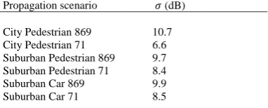
The standard deviation of the error between the measured data and associated fitted straight line model from Table 2 is shown in Table 3.

Table 3 Standard deviation of path loss model error

Propagation scenario (dB)

City Pedestrian 869 10.7 City Pedestrian 71 6.6 Suburban Pedestrian 869 9.7 Suburban Pedestrian 71 8.4

Suburban Car 869 9.9

Suburban Car 71 8.5

Results in [15] for 77.5 MHz propagation measurement in a hilly city, identified a distance-dependent coefficient of 46.4 (aligning well with our city pedestrian model) and a standard deviation of 8.6 dB. Our suburban car results are influenced by significant path loss variations in the small data set. However, shadowing and small-scale fading effects are quite usual in such field measurements and the standard deviation of the data (from the model straight lines) are not out of the ordinary, compared to other trials. The reduced distance-dependent term n of Table 2 may be due to the existence of several near LoS paths existing between the TX and some of the RX sites - even at the furthest range, which may not have existed in [15].

11 more favourable than in pedestrian scenarios, possibly due to

a more uniform azimuth coverage and improved gain at low elevation of the monopole above the car roof ground plane, compared to the hand-held whip or loop antenna. It is also interesting to note that for the suburban car scenario, coefficient n only varies between 25 and 26. Fixed loss term u can be closely represented by (8b) in the suburban car scenario, overall also supporting a simple propagation model.

9. Extracted Delay Profile Models

The CSR produces PDP time domain delay profiles which can be used to extract RMS delay spread. However, the lack of any observable reflections with delays significantly exceeding 1 µs has been remarkable during the field trials. This is in contrast with the findings of several others, as discussed in section 2, but perhaps does support the findings of [19], [20] and extends their applicability. During all the field trials, PDP data has been collected and examples showing close-in views of notable delay profiles on the correlation pulse are presented in Figs. 31–34. The PDPs produced during a conducted measurement are shown in Fig.

35 as a reference.

The PDPs produced from reference radiated measurements over a short range were also captured and found to be the same as in Fig. 35, apart for tests with the 71 MHz loop antenna. The reduced BW of the 71MHz loop antenna slews the PRBS bit transitions and extends the reference pulse, requiring a separate reference PDP for this setup, with 2 µs width at the -10 dB point.

a b

Fig. 31. 869 MHz City pedestrian channel response (47 m). (a) Close-in view of PDP, (b) Frequency response

a b

Fig. 32. 869 MHz Suburban pedestrian channel response

(107 m).

(a) Close-in view of PDP, (b) Frequency response

a b

Fig. 33. 71 MHz Suburban pedestrian channel response (414

m).

(a) Close-in view of PDP, (b) Frequency response

a b

Fig. 34. 71 MHz Suburban car channel response (107 m). (a) Close-in view of PDP, (b) Frequency response

a b

Fig. 35. Closein PDP from conducted measurement at

-90dBm (width of pulse at -10 dB point is 1.25 µs).

(a) 71MHz, (b) 869MHz

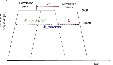
Given the low sample rate, care must be exercised in interpreting the close-in PDPs, when attempting to estimate the number of constituent rays and the delay spread. A small number of locations, such as Fig. 33a for example, do present what seems to resemble 2 PDP peaks. The approach taken in this section considers only the overall width of the recovered single PDP pulse, as a simplified method to estimate the RMS delay spread. By comparing the overall width of the obtained PDP correlation pulse at the -10 dB points to the width of the reference pulse at the -10 dB points, an estimation of the excess delay has been computed for those PDPs showing any pulse lengthening, as expressed in (9).

12 In (9), is 1.25 µs (2 µs for the 71MHz loop) and

is the width of the observed PDP pulse at the same point (i.e. -10dB point). The concept is illustrated in Fig. 36. Since the PRBS bit rate is 1 MHz and the RTL SDR sample rate is 2 MHz, the resolution of the PDP at low delay spreads is very limited, but it is still possible to extract some information. In general, the Mean Excess Delay can be expressed as [26]:-

(10)

is the level of the reflection’s correlation peak at delay Ti, relative to the primary ray. The second moment of the power delay can be expressed as [26]:-

(11)

The RMS delay spread can then be calculated from [26]:-

(12)

Since it was not possible, in general, to resolve the recovered CSR PDP data into distinct pulses, the simplifying model of 2 rays with the same amplitude has been used. Hence, the time separation between the ideal correlation peaks in the PDP is assumed to be the same as the measured difference in width of recovered pulse to reference pulse, D, as illustrated in Fig. 36.

It can then be shown that for this simple 2 ray case, the RMS delay spread simplifies to:-

(13)

Using the above approach, estimates of RMS delay spreads observed in all the measured data have been calculated and are presented in Table 4. However, it should be noted that in the majority of field measurements, no discernible spreading of the PDP correlation pulse was observed at the -10 dB width points. (The lowest discernible value of D observed in the measured data was 0.15 µs.)

Fig. 36. Extracting D from an assumed 2 ray PDP.

Table 4 Maximum and typical observed RMS delay spreads

Propagation scenario Maximum (µs)

Typical ranges (µs)

City Pedestrian 869 0.38 0 - 0.12 City Pedestrian 71 0.25 - Suburban Pedestrian 869 0.88 0 - 0.12 Suburban Pedestrian 71 0.5 0 - 0.25

Suburban Car 869 0.12 -

Suburban Car 71 0.38 0 - 0.12

10. Conclusions & Future Work

The combination of the R-Pi, RTL-SDR and Python DSP code have proved themselves as a valuable, novel system for performing propagation research measurements for modest cost and with high portability. This is important in facilitating focused use case propagation research in the field, allowing extraction of maximum insight at each location. This also allows the rapid evaluation of antenna concepts in the field. The proposed system is also applicable to the teaching of radio propagation; allowing students to witness the effects in near real-time, via the touchscreen.

In addition to the channel power delay response and frequency response, the CSR’s ability to calculate the path loss has allowed the creation of log-normal models for all the field trial scenarios. These extracted models have suggested that a basic 2 ray Reflective Earth distance-dependent model (augmented by a simple frequency-dependent loss term) may be pragmatic for pedestrian portable IoT use cases. A reduced distance-dependent coefficient appears sufficient to allow the model to also be used for the suburban car scenario, with more favourable path loss. The propagation model for suburban car at 71MHz is the most favourable.

It is surprising to note that no significant reflections with delays exceeding 1 µs have been observed, even with field test distances exceed 4 km over Sheffield’s hilly terrain. This suggests the reflective environment in both the city scenario and long-range urban scenario are only subject to reflections immediately adjacent to the primary path. However, the lack of strong reflections exceeding 1 µs does align with the findings of some other researchers as discussed in section 2. The estimated delay spreads based on the correlation pulse lengthening have shown maximum delay spreads below 1 µs. Most of the recovered spectrum profiles have been flat, with only a few examples of deep, wide fading nulls observed (mainly in 71MHz pedestrian operation).

Interference to CSR measurements was experienced in some of the test locations, at both 71 MHz and 869.525 MHz. This is suspected due to domestic and commercial switched mode PSUs, PC equipment and LTE band 20 signals. The CSR’s link budget is degraded by this interference, ideally requiring use of longer PRBS correlation sequences. This, in turn, would require more precise and stable oscillators at the TX and possibly within the CSR, at additional cost and complexity.

13 to capture channel measurements periodically over a longer

interval.

To increase both the RF carrier frequency and the

sounding bandwidth, our next CSR will replace the RTL-SDR with new bespoke RX RF front ends for sub 6 GHz and 28 GHz, coupled to a Red Pitaya FPGA board sampling IQ signals at 125 MHz (hence an effective RF bandwidth of 125 MHz). Additionally, a new companion high BW sounding transmitter will be used. The Red Pitaya will be both controlled and provide RX IQ signals to be analysed to the R-Pi. The R-Pi will implement the same DSP code and graphical interface as described in this paper. The future system will further enable valuable, portable propagation measurements to be performed cost-effectively for new bands of interest.

11. References

[1] Domazetović, B., Kočan, E., Mihovska, A.: ‘Performance evaluation of IEEE 802.11ah systems’. 2016 24th Telecommunications Forum (TELFOR), Belgrade, Serbia, Nov. 2016, pp. 1-4

[2] Lavric, A., Petrariu, A. L.: ‘LoRaWAN communication protocol: the new era of IoT’. 2018 International Conference on Development and Application Systems (DAS), Suceava, Romania, May 2018, pp.74-77

[3] Mroue, H., Nasser, A., Hamrioui, S., Parrein, B., Motta-Cruz, E., Rouyer, G.: ‘MAC layer-based evaluation of IoT technologies: LoRa, SigFox and NB-IoT’. 2018 IEEE Middle East and North Africa Communications Conference (MENACOMM), Lebanon, Lebanon, April. 2018, pp. 1-5 [4] Ofcom, ‘VHF radio spectrum for the Internet of Things (Statement)’. 2016.

[5] Bagal, S., Desai, P., Gulavani, A., Patil, R. A.: ‘Considerations for wireless communication at 868MHz’. 2014 Annual IEEE India Conference (INDICON), Pune, India, Dec. 2014, pp. 1-5

[6] Ball, E. A.: ‘Portable and low cost channel sounding platform for VHF / UHF IoT propagation research’. Loughborough Antennas & Propagation Conference (LAPC 2017), Loughborough, UK, November 2017, pp.1-5 [7] Stewart, J., Stewart, R., Kennedy, S.: ‘Internet of Things – propagation modelling for precision agriculture applications’. 2017 Wireless Telecommunications Symposium (WTS), Chicago, USA, April. 2017, pp. 1-8 [8] Allsebrook, K., Parsons, J. D.: ‘Mobile radio propagation in British cities at frequencies in the VHF and UHF bands’, IEEE Trans. on Vehicular Technologies, 1977, 26, pp. 313-323

[9] Vigneron, P. J., Pugh, J. A.: ‘Propagation models for mobile terrestrial VHF communications’. MILCOM Conference, San Diego, USA, Nov. 2008, pp. 1-7

[10] Hata, M..: ‘Empirical formula for propagation loss in land mobile radio services’. IEEE Trans. on Vehicular Technology, 1980, 29, (3), pp. 317-325

[11] Dagefu, F. T., Verma, G., Rao. C. R., et al., ‘Measurement and characterization of the short-range low-VHF channel’. WCNC Conference, New Orleans, USA, March 2015, pp. 177-182

[12] Pugh, J. A., Bultitude, R. J. C., Vigneron, P. J.: ‘Mobile propagation measurements with low antennas for segmented wideband communications at VHF’. 12th ANTEM Conference, Montreal Canada, July 2006, pp. 1-4

[13] Fischer, J., Grossmann, M., Felber, W., Landmann, M.: ‘A novel delay spread distribution model for VHF and UHF mobile-to-mobile channels’. 2013 7th European Conference on Antennas and Propagation (EuCAP), Gothenburg, Sweden, April 2013, pp. 469-472

[14] Pugh, J. A., Bultitude, R. J. C., Vigneron, P. J.: ‘Propagation measurements and modelling for multiband communications on tactical VHF channels’. MILCOM 2007 - IEEE Military Communications Conference, Orlando, USA, Oct. 2007, pp 1-7

[15] Bedeer, E., Pugh, J., Brown, C., Yanikomeroglu, H.: ‘Measurement-based path loss and delay spread propagation models in VHF/UHF bands for IoT communications’. 2017 IEEE 86th Vehicular Technology Conference, Toronto, Canada, Sept. 2017, pp. 1-5

[16] Karam, M., Turney, W., Baum, K. L., et al.: ‘Outdoor-indoor propagation measurements and link performance in the VHF/UHF bands’. 2008 IEEE 68th Vehicular Technology Conference, Calgary, Sept. 2008, pp.1-5 [17] Safer, H., Berger, G., Seifert, F.: ‘Wideband propagation measurements of the VHF-mobile radio channel in different areas of Austria’. 5th International Symposium on Spread Spectrum Techniques and Applications, Sun City, South Africa, Sept. 1998, pp. 502-506

[18] Sasaki, M., Yamada, W., Sugiyama, T.: ‘VHF band path loss model for low antenna heights in residential areas’. The 8th European Conference on Antennas and Propagation (EuCAP 2014), The Hague, Netherlands, April 2014, pp. 2092-2094

[19] Sizov, V., Gashinova, M., Zakaria, N., Cherniakov, M.: ‘VHF communication channel characteristics over complex wooded propagation paths with applications to ground wireless sensor networks’, IET Microw. Antennas Propag., 2013, 7, (3), pp. 166-174

[20] Dagefu, F. T., Verma, G., Rao, C. R., et al.: ‘Short-range low-VHF channel characterization in cluttered environments’, IEEE Trans. On Antennas and Propag., 2015, 63, (6), pp. 2719-2727

[21] Fannin, P. C., Molina, A., Swords, S. S., Cullen, P. J.: ‘Digital signal processing techniques applied to mobile radio channel sounding’. IEE Proceedings F - Radar and Signal Processing, 1991, 138, (5), pp. 502-508

[22] Charles, S. A., Ball, E. A., Whittaker, T. H., Pollard, J. K.: ‘Channel sounder for 5.5GHz wireless channels’. IEE Proceedings in Communications, 2003, 150, (4), pp. 253-258 [23] MacCurdy, M., Gabrielson, R., Spaulding, E., et al.: ‘Automatic animal tracking using matched filters and time difference of arrival’. Journal of Communications, 2009, 4, (7), pp. 487-495

[24] Landa, I., Blázquez, A., Vélez, M., Arrinda, A.: ‘Indoor measurements of IoT wireless systems interfered by impulsive noise from fluorescent lamps’. 11th European Conference on Antennas and Propagation (EUCAP), Paris, France, May 2017, pp. 2080-2083

[25] Balanis, C. A.: ‘Antenna Theory’ (Wiley Interscience, 3rd _{Edition, 2005)}