An incremental approach to the solution of global trajectory optimization problems

Vasile, M. and Ceriotti, M. and De Pascale, P. (2007) An incremental approach to the solution of

global trajectory optimization problems. In: Advances in Global Optimization: Methods and

Applicaitons, 13-17 June 2007, Mycanos, Greece.

http://

strathprints

.strath.ac.uk/

20168

/

This is an author produced version of a paper published in Advances in Global Optimization:

Methods and Applicaitons, 13-17 June 2007, Mycanos, Greece. This version has been peer-reviewed

but does not include the final publisher proof corrections, published layout or pagination.

Strathprints is designed to allow users to access the research output of the University

of Strathclyde. Copyright © and Moral Rights for the papers on this site are retained

by the individual authors and/or other copyright owners. You may not engage in

further distribution of the material for any profitmaking activities or any commercial

gain. You may freely distribute both the url (

http://

strathprints

.strath.ac.uk

) and the

content of this paper for research or study, educational, or not-for-profit purposes

without prior permission or charge. You may freely distribute the url

(

http://

strathprints

.strath.ac.uk

) of the Strathprints website.

An incremental approach to the solution of global

trajectory optimization problems

Massimiliano Vasile • Matteo Ceriotti • Paolo De Pascale

Abstract This paper presents an incremental approach to the solution of multiple

gravity assist trajectories (MGA) with deep space maneuvers. The whole problem is decomposed in problems that are solved incrementally. The solution of each sub-problem leads to a progressive reduction of the search space. Unlike other similar methods, the search for solutions of each sub-problem is performed through a stochastic approach. The resulting set of disconnected boxes is transformed into a connected collection of boxes through an affine transformation. For MGA problems, the incremental approach increases both the efficiency and reliability of the optimization process. Two relevant examples will illustrate the effectiveness of the proposed method.

Keywords Trajectory optimization · Branch and prune · Multi-gravity assist

trajectories

1Introduction

In recent times there has been a flourishing interest in methods and tools for preliminary mission analysis and design, ranging from low-thrust trajectory design [2, 4], to perturbed geocentric orbits [3], to multiple gravity assist trajectories [10, 11, 13]. In particular, the generation of a large number of mission alternatives that can serve as first guesses for more detailed and sophisticated analyses.

M. Vasile () · M. Ceriotti

Department of Aerospace Engineering

University of Glasgow, James Watt Building (South) Glasgow, G12 8QQ, United Kingdom

e-mail: [email protected]

P. De Pascale

This interest is directly related to the modern approach to space mission design, which steps through phases of increasing complexity, the first of which is always a mission feasibility study. In order to be successful, the feasibility study phase has to analyze, in a reasonably short time, a large number of different mission options. Each mission option requires the design of one or more optimal trajectories. In mathematical terms, the problem can be seen as a global optimization or as a global search for multiple local minima.

A typical example is the optimization of multiple gravity assist trajectories (MGA). In this case a spacecraft exploits the encounter with one or more planets in order to change its velocity vector [8]. For an accurate trajectory model, the number of alternative paths can grow exponentially with the number of encounters. Moreover, finding an optimal planet-to-planet transfer is, in itself, a global optimization problem, due to the high number of local minima.

Solving the problem could be a challenge for every global optimization tool. However, this class of global trajectory optimization problems can be decomposed into sub-problems of smaller complexity and solved incrementally adding one planet at the time. At each incremental step, a portion of the search space can be pruned out. Previous attempts to use an incremental pruning have employed a simplified trajectory representation and a grid sampling of each sub-problem [9]. This approach fails if the accuracy and complexity of the trajectory model are increased, for two reasons: if a course grid and an aggressive pruning are used, many optimal solutions are lost; on the other hand, if a fine grid is used, the computational time becomes unacceptable even for a limited number of planets.

The solution of the MGA problem was already tackled and solved for some specific cases with a hybrid stochastic-deterministic optimizer for black-box problems [13]. In this work, it is proposed a problem dependent approach, in which the grid sampling is substituted with a global search through a stochastic method. Each global search aims at finding not only the global optimum, but also a number of local optima. Then, the neighborhood of each local optimum is preserved and the rest of the search space is pruned out. It will be shown how the proposed stochastic search performs an efficient and reliable global optimization of the whole trajectory. This approach will be compared to the direct application of known stochastic and deterministic global optimization tools.

2Global optimization of multi-gravity assist trajectories

A multi-gravity assist trajectory (MGA) can be defined as a sequence of transfer arcs and swing-bys of gravitational bodies, starting from a departure one to a target one (or a target orbit). Along the transfer arcs, the engine of the spacecraft can be fired to produce a minor change in its velocity vector. Each swing-by, instead, exploits the gravity of the celestial body to produce a major change in the velocity of the spacecraft.

not change, and coincides with the position of the celestial body at the time of the swing-by, in the case of a gravity assist maneuver.

In other words, each maneuver has the effect of introducing a discontinuity in the velocity vector, but not in the position vector. The propelled maneuvers are called deep space maneuvers (DSM) and the generic change in velocity Δv. This particular model of a multi-gravity assist trajectory is called linked-conic approximation since it is made of conic arcs (the transfer arcs) linked together by impulsive changes in the velocity vector (given by the swing-bys).

For each instant of time the position and velocity of the celestial bodies is given by analytical ephemerides, with respect to a heliocentric, ecliptic, inertial reference frame. Therefore, given a sequence of celestial bodies and times of encounter, the position of each gravity assist maneuver is fully determined. For the case under examination, all the celestial bodies are planets. At the departure planet, the velocity of the spacecraft is the sum of the launch velocity and the heliocentric velocity of the planet and is normally limited by the launch capabilities.

2.1Gravity assist model

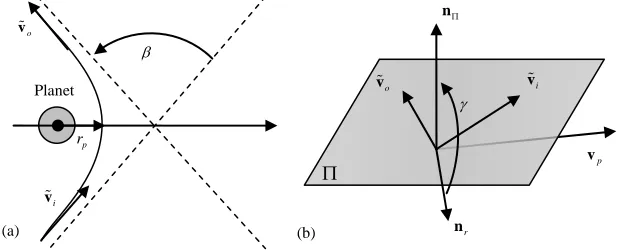
As mentioned above, the effect of the gravity of a planet is to instantaneously change the velocity vector of the spacecraft. The relative incoming velocity vector and the outgoing velocity vector, at the planet swing-by, have the same modulus but different directions; therefore the heliocentric outgoing velocity results to be different from the heliocentric incoming one. The angular difference β between the incoming relative velocity _i and the outgoing on v_%o depends on the modulus of the incoming velocity and on the minimum distance from the center of the planet, or peric ntre r rp [8] (Fig. 1a). In the linked conic model the spacecraft is assumed to follow a

hyperbolic trajectory with respect to the swing-by planet. Both the relative incoming and outgoing velocities belong to the plane of the hyperbola. However in the linked-conic approximation the maneuver is assumed to occur at the planet, where the planet is a point mass coinciding with its center of ma

v_% e

e

ss. adius,

Therefore, given the incoming velocity vector, one angle is required to define the attitude of the plane of the hyperbola Π. There are different possible choices for the attitude angle γ; the one proposed in [14] has been adopted (Fig. 1b): γ is the angle between the normal vector nΠ to the hyperbola plane Π and the reference vector nr

o v%

β

Planet

p

r

i v%

(a)

Π

r n Π n

p v i v% o

v

%

γ

(b)

that is normal to the plane containing the incoming relative velocity and the velocity of the planet vp.

2.2Trajectory Model and Problem Formulation

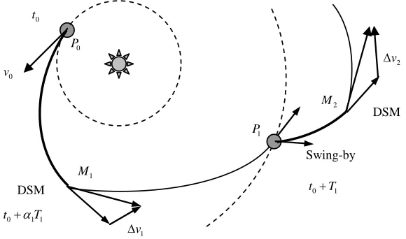
A complete MGA trajectory is divided into a number of phases connecting a sequence of celestial bodies (the full trajectory model is represented in Fi ). Given a sequence of

g. 2

P

N planets, there exist k=1,...,N_P−1 phases, each of them beginning and ending with an encounter with a planet. Each phase k is made of two conic arcs: the first, propagated analytically forward in time, ends where the second, solution of a Lambert’s problem [1], begins. The two arcs have a discontinuity in the absolute heliocentric velocity at their matching point Mk. Each DSM is computed as the vector

difference between the velocities along the two conic arcs at the matching point Mk.

Given the transfer time Tk, relative to each phase k and the variable αk =

[ ]

matching point is at time tDSM k, =tf k, −1+αkTk, where tf k, −1 is the final time of the

phase . The velocity vector at the departure planet can be a design parameter and is expressed as:

1

k−

[

]

0 0 sin cos , sin sin , cos

T

v δ θ δ θ δ

=

v (1)

with the angles δ and θ respectively representing the declination and the right ascension with respect to a local reference frame with the x axis aligned with the velocity vector of the planet, the z axis normal to orbital plane of the planet and the y

axis completing the coordinate frame. This choice allows easily constraining the escape velocity and asymptote direction while adding the possibility of having a deep space maneuver in the first arc after the launch. This is often the case when escape velocity must be fixed due to the launcher capability or to the requirement of a resonant swing-by of the Earth (Earth-Earth transfers). Alternatively it is possible to use a simpler model in which the first leg from P₀ to P₁ is a simple Lambert’s arc

0

P

1

v

Δ

0

v

Swing-by 0

t

0 1

t +T

0 1 1

t +αT

1

P

1

M

DSM

2

M

2

v

Δ

DSM

with no deep space maneuver. In this case the departure velocity is computed a posteriori and the number of optimization parameters and degrees of freedom are reduced. This simpler version of the model is suitable for the assessment of sequences that fly directly to another planet after launch.

Once the heliocentric velocity at the beginning of phase k, which can be the result of a swing-by maneuver or the asymptotic velocity after launch, is computed, the trajectory is analytically propagated until time tDSM k, . The second arc of phase k is

then solved through a Lambert’s algorithm, from Mk, the Cartesian position of the

deep space maneuver, to , the position of the target planet of phase k, for a time of

flight . Two subsequent phases are then joined together using the swing-by model. The complete solution vector for this model is:

k

P

(

)

(2)

0, , , , ,0 1 1, 1, p,1,..., k, k, k, p k, ,..., NP 1, NP

v θ δ t T α γ r T α γ r T ₋ α ₋

⎡ ⎤

= ⎣ ⎦

x ₁

where is the departure date. Now, the design of a multi-gravity assist transfer can be transcribed into a general nonlinear programming problem, with simple box constraints, of the form:

0

t

min ( )

with

f

D

∈

x x

x

(3)

One of the appealing aspects of this formulation is its solvability through a general global search method for box constrained problems. Depending on the kind of problem under study the objective function can be defined as:

( )

1

p

P N

k N

k

f

−

∞

=

= +

∑

x v v v (4)

In the following the relative velocity at the target planet

P N

∞

v will not be included in the objective function.

3An incremental approach

For a function f x

(

)

the global minimum problem can be formulated in the following way:

( )

0: min

D

P f

∈

x x (5)

where D is an n-dimensional hyper-rectangle defining the search space. In some cases the solution vector for has to be ordered according to a temporal criterion. This can

occur when

0

P

( )

f x is the result of an algorithm. In this case the value of f cannot be computed by assigning values to the components of in an arbitrary order. Although all the components are independent and therefore the problem cannot be reduced, the computation of the function f must follow a precise order. Thus Eq.

x

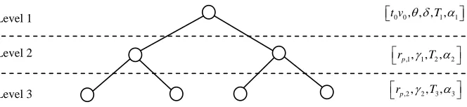
assumes different values depending on the path followed along the graph. Each node can be seen as an independent sub-problem into which can be decomposed, provided that all the preceding sub-problems are solved following a prescribed order. In some special cases, all the problems can be solved in an arbitrary order provided that the value of the function f is computed following the direction of the graph. If problem can be decomposed into m sub-problems that can be solved independently and the value f can be computed as the ordered sum of all the values of all the sub-problems, following the oriented graph, then the problem can be solved incrementally moving along the graph from top to bottom or from bottom to top as shown in . Each sub-problem i is defined on a dimensional slice of D such

that .

0

P

0

P

0

P

Level 1

Level 2

Level 3

,1, ,1 2, 2

p

r γ T α

⎡ ⎤

⎣ ⎦

0 0, , , ,1 1 t v θ δ T α

⎡ ⎤

⎣ ⎦

,2, 2, 3, 3

p

r γ T α

⎡ ⎤

⎣ ⎦

Fig. 3 Tree representation of a MGA trajectory: each node is a stage composing the trajectory

Fig. 3

Fig. 3

i

D

1 2 ... i... m

D=D×D × D ×D

The solution time is the sum of the individual solution times of each sub-problem plus the time to add up all the output values of all the sub-problems by following all the feasible paths along the oriented graph. The incremental solution of problem offers the interesting possibility of reducing the search space D by redefining the size of each slice once the i-th sub-problem has been solved. This means that, even if the problem complexity grows exponentially with problem dimensions, the solution time can be reduced to acceptable numbers.

0

P

i

D

3.1Branch and prune process

Each node of the graph shown in is defined by a value assigned to a subset of . For example, in Fig. 3, the solution vector x has been decomposed into two solution vectors assigned to level 1 and level 2 respectively. Each group of nodes represents a level of the tree. The tree can be branched by systematically decomposing each sub-domain into boxes, such that:

x

i

D q_i

(6)

, 1

i q

i _j

D =

U

The number of nodes per level depends on the number of boxes. Now a number of criteria can be defined to decide whether to prune or to keep one of the boxes at a given level i. In general, a function fi

(

)

Furthermore, since the evaluation of f has to follow a path along the ordered tree composed of connected nodes, the space reduction, or pruning, at a given level i

be evaluated is

1

m q

i

m

=

=

∏

avoid an exponential growth of the number of evaluations. Moreover, the correct evaluation of each box depends on its size and therefore on . If, on the other hand, each node can be decoupled from the others, it can be demonstrated that the complexity of the problem grows polynomially with the number of levels [9]. After the pruning of level i, the feasible domain of the objective function

,

i j

D q_i

f will be:

1 2 ... i i 1 ...

D=D ×D × ×D ×D₊ × ×D_m (7)

where Di is the pruned sub-domain at level i. Then, it may be possible to consider

another function fi+1 and evaluate it on the non-pruned part of all the sub-domains up

to Di+1. The pruning process continues up to the last level m, at which, the actual

function f can be evaluated.

The proposed incremental approach aims, for each level i, at the identification of the basin of attraction of the local optima for the pruning criterion fi. Once the basin

is identified, an enveloping box (or a cluster of boxes) is created around it. Only the solution space within the boxes is preserved and the rest of the solution space at level i

is pruned out. If the pruning criteria are chosen properly, the local optima, and the global optimum, of the objective function f are included in the collection of all the boxes generated at each of the m levels.

3.2Box collection and affine transformation

Although the space reduction improves the computing time, the number of boxes could grow exponentially, if every combination of boxes at each level is considered. A possible solution is to collect all the boxes at each level and sample (or search) the collection instead of each single box individually. The boxes generated at each level i

are generally disconnected, therefore it has been applied a space transformation that maps all the disconnected boxes into a unit hypercube made of connected boxes. The dimensionality of the transformed space is the same as the one of the original space, so is the number of connected boxes in the unit hypercube.

An affine transformation is then used to map each point x in the unit hypercube into a point x in the real space:

(

)

(

)(

)

, ,

u j l j

j j l

u j l j

b b

,

j u j

x x b b

b b

−

= −

− + (8)

for each dimension j of the level under consideration. b bu, l are the upper and the

lower bounds of the box in the unit hypercube which contains x, and are the bounds of the corresponding box in the real space.

,

u l

b b

The value of the pruning function fi at level i is then evaluated by sampling the

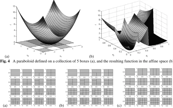
affine space for levels 1 and then mapping the sampled points into the real space. It should be noted that the objective function seen from the affine space is discontinuous even if it is continuous in the real space ( ). This strongly depends on how the boxes are connected in the affine space. However, if the boxes are

,...,i

disconnected or overlapped in the real space, the objective function in the affine space results to be always discontinuous. In addition the number of local minima in the affine space may be larger than in the real space. Although this might seem a pitfall, it should be noted that in practice a good deal of the minima in the affine space are replica of few minima in the real space. As a consequence there is an increased probability to find a good solution.

In order to preserve the same probability of sampling a point in each box of the real space, the partitioning of the unit hypercube should be made in such a way that all the boxes have the same size, and the number of subdivisions along each coordinate is the same. Being the number of dimensions of the generic level i, and the number of boxes on that level, it is possible to meet these two requirements together only if:

i

d q_i

i d

i

t= q

is an integer. t is the number of intervals to consider on each dimension to partition the affine space into hyper-cubes. In all the other cases, it is always possible to have boxes of equal size (for example cutting the hypercube along only one coordinate), but the number of subdivisions per coordinate would be uneven.

i

q

In general, there are infinite ways to partition the affine space in a given number of boxes. Some of them have been analyzed and implemented in this work. Fig. 5 shows how three different algorithms partition the unit hypercube, in a 2-dimensional case. Solution (c) has been chosen for this work, as it is the one which provides regular boxes in most of the cases. The difference is noticeable for 3, 6, 8, 12, 15 boxes. However, the generation of boxes in the real space is arbitrary therefore it is always possible to generate the optimal number of boxes.

(a) (b) (c)

Fig. 5 Three different ways to partition the affine space (in a 2-dimensional case) for a required number of

boxes from 1 to 16

(a) (b)

4Results

The incremental approach was tested on two basic problems with a single gravity assist maneuver: an Earth-Venus-Mars transfer and an Earth-Earth-Mars transfer. Despite the simplicity of these two test cases they are representative of two classes of MGA transfers and well illustrate the complexity of these kinds of problems.

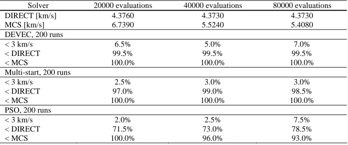
The incremental approach was compared to the direct solution of the whole problem (all-at-once approach) with five different global optimization methods, two deterministic and three stochastic. The two deterministic optimizers are DIRECT (Divided Rectangles, [6]) and MCS (Multilevel Coordinate Search, [5]). The stochastic optimizers are DEVEC, an implementation of Differential Evolution [12], PSO, an implementation of Particle Swarm Optimization [7], and a simple multi-start, which takes a suitable number of samples in the search space and optimizes the best one locally by using Matlab® fmincon. The optimizers were applied with different settings and with an increasing number of function evaluations. In the following, the optimizers are tested for 20000, 40000 and 80000 function evaluations.

The incremental approach uses at each level a random sampling of the solution space with Latin Hypercube, and then runs a local optimization from each sample. The local search is performed by using fmincon. In both test cases the whole problem is decomposed into two levels. After a set of minima for level 1 is found and a set of boxes is generated, the affine transformation is applied to the subspace at level 1 and the incremental approach proceeds by adding the second level.

4.1EVM transfer

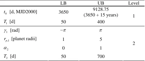
The first test case consists of a transfer from the Earth to Mars exploiting a swing-by of Venus. For this test, a simpler version of the trajectory model was used, with no DSM along the Earth-Venus transfer leg. Therefore the problem has dimension 6 and the bounds of the search space are reported in Table 1.

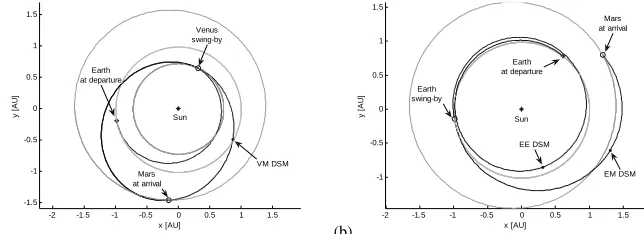
Level 1 computes the first deep space flight phase, while the second adds the swing-by of Venus and the deep space flight to Mars. The objective function f is the total , which is the sum of the relative velocity at departure and the DSM between Venus and Mars. The problem was initially analyzed by running a multi-start on the whole domain. A local search was started from a total of 500 starting points, taken with Latin Hypercube, and the 10 best solutions are shown in . The total number of function evaluations needed to compute all the solutions was 494233. The trajectory corresponding to the best solution is shown in

v

Δ

Table 2

Fig. 9a.

Table 1 Bounds for the EVM test case

LB UB Level

9128.75 (3650 + 15 years) 0

t [d, MJD2000] 3650

1

T [d] 50 400

1

π

− π

[rad] 1

γ

,1 p

r [planet radii] 1 5

2

α 0 1 2

2

The three stochastic global optimizers mentioned above were run on the whole problem for 200 consecutive times. In Table 3 it has been reported the percentage of times the stochastic optimizer finds a solution proximal to solution 1 in . In addition we report the percentage of times the stochastic optimizers find a solution that is better than the deterministic ones. The key point in the proposed incremental approach is not only to reduce the computational cost but also to increase robustness, i.e. increase the probability to find the global minimum.

Table 2

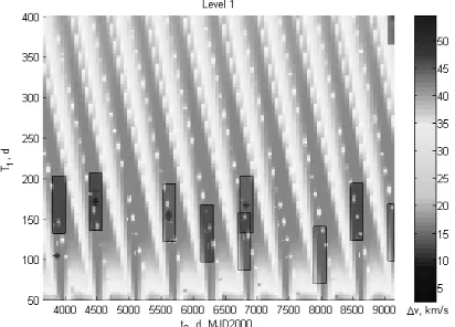
The incremental approach starts at level 1 by looking for all local minima for the objective function f₁ which is the departure relative velocity at the Earth. A local search was started from a total of 20 random starting points and an equal number of boxes were generated. Fig. 6 shows the contour plot of the search space at level 1. The boxes which have been generated by the algorithm are highlighted in dark grey, in semi-transparency. The size of the boxes is arbitrary and was set to a percentage of each dimension.

The multi-start search of the incremental algorithm was able to identify almost one local minimum for each sinodic period. The number of evaluations to find all the 20 boxes was 516. After applying the affine transformation to level 1 and adding level 2, the whole reduced space was sampled with other 20 random starting points, and a local

Table 3 Solutions and performances of different optimizers on the EVM transfer

Solver 20000 evaluations 40000 evaluations 80000 evaluations

DIRECT [km/s] 4.3760 4.3730 4.3730

MCS [km/s] 6.7390 5.5240 5.4080

DEVEC, 200 runs

< 3 km/s 6.5% 5.0% 7.0%

< DIRECT 99.5% 99.5% 99.5%

< MCS 100.0% 100.0% 100.0%

Multi-start, 200 runs

< 3 km/s 2.5% 3.0% 3.0%

< DIRECT 97.0% 99.0% 98.5%

< MCS 100.0% 100.0% 100.0%

PSO, 200 runs

< 3 km/s 2.0% 2.5% 7.5%

< DIRECT 71.5% 73.0% 78.5%

< MCS 100.0% 96.0% 93.0%

Table 2 The 10 best solutions found with the all-at-once approach for the EVM problem

,1 p

r

[radii] 0

t γ1

[d, MJD2000] [rad]

v Δ

[km/s] T1 [d] α2 T2 [d]

Sol.

1 2.9818 4472.013 172.2893 2.9784 1 0.5094 697.61

2 2.983 4473.775 170.5335 2.9859 1.0005 0.8611 698.1473

3 2.9962 4475.217 171.1191 2.853 1.076 0.7292 692.8782

4 3.0393 4480.19 167.5824 2.8044 1.1307 0.6371 692.5669

5 3.1707 4482.079 174.6522 -2.8195 1.1885 0.4608 629.9262

6 3.1708 4482.145 174.6048 -2.822 1.2033 0.4923 629.7778

7 3.1719 4481.964 174.7837 -2.8076 1.106 0.6224 630.7661

8 3.1884 4471.355 171.4453 -3.1416 1.019 0.5334 700

9 3.2217 3872.306 105.6978 2.7087 1 0.545 628.0203

search was run from each one of them for a total of 8827 function evaluations. The result was that:

Fig. 6 Boxes found after analyzing level 1. The space outside the boxes is pruned. The background gives

an idea of the distribution of the local minima

• 90% of the 20 best solutions found with the all-at-once approach have the values of level 1 variables included in one of the boxes;

• The best solution found with the incremental approach is the same as the best known solution, i.e. solution 1 in Table 2.

In addition, the incremental search has been run twenty consecutive times, obtaining always the same result and the same global minimum.

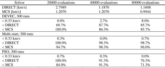
4.2EEM

The second test case consists of an Earth to Mars transfer, through a swing-by of the Earth. This second case is significantly more complicated than the previous one due to the required optimization of the Earth-to-Earth transfer in order to design a correct gravity assist maneuver. The Earth gravity assist is used to increase the kinetic energy of the spacecraft with respect to the Sun when the launch capabilities are limited. In order to gain the required Δv, the spacecraft has to reach the Earth with a relative velocity vector different from the one at departure. Thus, a targeting DSM is required along the Earth-Earth transfer leg. The departure velocity vector depends on the launch capabilities therefore its modulus was set at 2 km/s for this test case, while the declination δ and right ascension θ were left free. Table 4 presents the boundaries for the variables of the problem. Once again the whole problem is decomposed into two sub-problems, corresponding to two levels. Level 1 consists of the Earth-Earth transfer, while level 2 computes the swing-by and the Earth-Mars transfer leg. The objective function f is the sum of the Δv of the two deep space maneuvers.

Due to the higher dimensionality of this test, 5000 starting points were used, leading to about function evaluations. The 10 best solutions are shown in

, and the globally optimum trajectory is represented in

6

9 10⋅ Table

5 Fig. 9b. As in the previous

Table 4 Bounds for the EEM test case

LB UB Level

9128.75 (3650 + 15 years) 0

t [d, MJD2000] 3650

π

− π

[rad] δ

1 2

π

− π 2

θ [rad]

1

α 0.01 0.99

1

T [d] 50 1000

π

− π

[rad] 1

γ

,1 p

r [planet radii] 1 5

2

α 0 1

2

2

T [d] 50 1000

Table 5 The 10 best solutions found with the all-at-once approach for the EEM problem

,1 p

r

[radii] 0

t [d, T1 T2

MJD2000] [d]

v

Δ

[km/s]

δ

[rad]

θ

[rad] α1

1

γ

[rad] 2 [d]

α

0.326 5430.17 -1.883 -0.0031 0.4691 500.065 -2.901 2.937 0.6195 307.900

0.333 6184.04 1.358 0.0266 0.5171 524.750 3.142 3.022 0.4186 244.296

0.346 3650.00 1.341 -0.0032 0.4552 514.730 -2.982 4.438 0.4666 706.343

0.350 3770.54 1.789 0.025 0.2607 383.198 2.875 2.414 0.6642 711.414

0.361 6318.71 1.793 -0.0642 0.2623 383.977 2.749 2.833 0.0288 207.888

0.361 8732.38 -1.768 -0.0018 0.6846 888.721 3.142 3.860 0.7118 766.862

0.368 6323.20 -1.446 0.0083 0.3073 385.862 -3.084 2.758 0.1549 242.328

0.374 6322.99 -1.446 0.0032 0.3163 387.371 3.119 2.815 0.1556 243.481

0.376 5031.64 -1.774 0.0079 0.6778 886.791 -2.800 4.173 0.3367 304.612

0.378 5029.72 -1.774 0.0115 0.679 887.477 -2.762 4.046 0.228 302.372

Table 6 Solutions and performances of different optimizers on the EEM transfer

Solver 20000 evaluations 40000 evaluations 80000 evaluations

DIRECT [km/s] 2.7989 1.1870 1.1608

MCS [km/s] 1.2070 1.2070 0.9944

DEVEC, 300 runs

< 0.33 km/s 0.0% 2.7% 8.0%

< DIRECT 69.7% 87.7% 85.7%

< MCS 100.0% 86.3% 85.7%

Multi-start, 300 runs

< 0.33 km/s 0.3% 0.0% 0.7%

< DIRECT 100.0% 98.3% 98.7%

< MCS 94.7% 98.3% 96.0%

PSO, 300 runs

< 0.33 km/s 0.7% 0.3% 0.0%

< DIRECT 100.0% 91.3% 76.3%

The choice of the objective function f₁ for the incremental approach is trickier than in the previous case. In fact if the sum of the DSM and of v0 is chosen, the

optimizer returns solutions with no maneuver at all. Furthermore, it is known from the physics of the problem that the zero-maneuver solution is a local minimizer even for the whole EEM transfer. Since the gravity assist maneuver requires an accurate timing to reach the swing-by planet with the right incoming conditions, its effect is to narrow down the basin of attraction of each minima. Now a zero-maneuver solution for the EEM case physically corresponds simply to a delayed departure from Earth after the EE leg, with no gravity assist. All the zero-maneuver solutions, therefore, have a much wider basin of attraction.

This can be easily verified by applying a general stochastic global optimizer to the whole EEM problem. The optimizer will return with a higher probability the zero-maneuver solutions if no special condition is imposed on the departure velocity at the Earth. In order to minimize the Δv on the EM leg, the incoming velocity vector at the Earth should be as such to have an outgoing relative velocity vector aligned with the velocity vector of the Earth (maximum increase in the kinetic energy).

A suitable criterion to optimize the first leg can be found by studying the characteristics of the relative velocity vector at the end of the Earth-Earth transfer.

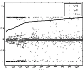
represents the in-plane components (radial and transversal) of the normalized incoming relative velocity vector for the best solutions found with the all-at-once approach. On the same plot the objective function for the complete problem is also represented.

Fig. 7

For the best solutions (from 1 to about 300), the direction of the relative velocity is almost completely radial. Therefore, we took the following function as pruning criterion:

2 2

1 2

h r

v v

f v

v

θ +

= + Δ (9)

which tries to minimize the DSM while maximizing the radial component of the relative velocity before the swing-by, with respect to the other components. Although this criterion was derived for a specific case, it has general validity and applies to two classes of MGA transfers: aphelion rising gravity maneuvers and perihelion lowering gravity maneuvers.

Fig. 7 Normalized in-plane components of the incoming relative velocity vector before the Earth swing-by,

The incremental approach was applied to level 1 starting a local search from 60 random points for a total of 13547 function evaluations. Unlike in the previous case, the edges of the boxes on all the dimensions are a reasonable fraction of the search space, except for the edge along direction , which spans the entire range. The reason is that the orbit of the Earth is almost circular: therefore a different position along its orbit has little influence on the arrival conditions at the end of the Earth-Earth leg.

0

t

Fig. 8a and Fig. 8b show the projection of the boxes along variables of level 1. The red starts represent the 50 best solutions found with the all-at-once approach. After applying the affine transformation to level 1 and adding level 2, the reduced search space was sampled with 30 points and a local optimization was started from each one of them for a total of 32544 function evaluations. The result was that:

• 86% of the 50 best solutions found with the all-at-once approach have the values of the level 1 variables included in one of the boxes;

• The best solution found with the incremental approach is the same best solution in the table.

Even in this case, the incremental approach was run for 20 times obtaining always the same result.

(a) (b)

Fig. 8 Projection of the boxes in level 1 along the direction of the variables t0, ,δ θ (a) and (b). The

stars are the 50 best all-at-once solutions

1,T1

α

(a)

-2 -1.5 -1 -0.5 0 0.5 1 1.5 -1.5

-1 -0.5 0 0.5 1 1.5

x [AU]

y [

A

U

]

Sun Earth

at departure

Venus swing-by

VM DSM Mars

at arrival

(b)

-2 -1.5 -1 -0.5 0 0.5 1 1.5 -1

-0.5 0 0.5 1 1.5

x [AU]

y [

A

U

]

Earth at departure

Mars at arrival

Earth swing-by

Sun

EE DSM

EM DSM

5Conclusion

In this paper we presented an incremental approach for the solution of multi-gravity assist trajectory with deep-space maneuvers. The approach is based on a decomposition of the whole problem in sub-problems that can be solved incrementally. For each sub-problem, a stochastic optimization approach is used to identify the basin of attraction of the local optima with respect to a pruning criterion. Then, a portion of the basin of attraction is enveloped in a set of boxes and the rest of the search space is pruned out. Equivalently it is possible to look for the feasible set according to the pruning criterion. After pruning, the remaining search space for each sub-problem is made of a disconnected set of boxes. An affine transformation is then applied to generate a connected and compact collection of boxes.

The proposed approach has demonstrated to be reliable and efficient compared to the solution of the whole problem all-at-once. In particular the incremental approach provides a significant reduction in the number of function evaluations compared to deterministic methods and an increased reliability compared to standard stochastic approaches. The present implementation makes use of a simple multi-start search. A more effective sampling approach would require the use of a more sophisticated global optimizer and a clustering of all the feasible points according to each pruning criterion.

References

1. Battin, R.H.: An introduction to the mathematics and methods of astrodynamics, revised edition. AIAA Education Series. AIAA, New York (1999)

2. Dachwald, B.: Optimization of Interplanetary Solar Sailcraft Trajectories Using Evolutionary Neurocontrol. Journal of Guidance, Control, and Dynamics 27(1), 66-72 (2004)

3. Gurfil, P., Kasdin, N.J.: Niching genetic algorithms-based characterization of geocentric orbits in the 3D elliptic restricted three-body problem. Computer Methods in Applied Mechanics and Engineering

191(49-50), 5683-5706 (2002)

4. Hartmann, J.W., Coverstone-Carroll, V.L., Williams, S.N.: Optimal interplanetary spacecraft trajectories via a Pareto genetic algorithm. Journal of the Astronautical Sciences 46(3), 267-282 (1998) 5. Huyer, W., Neumaier, A.: Global optimization by multilevel coordinate search. Journal of Global

Optimization 14(4), 331-355 (1999)

6. Jones, D.R., Perttunen, C.D., Stuckman, B.E.: Lipschitzian optimization without the Lipschitz constant. Journal of Optimization Theory and Applications 79(1), 157-181 (1993)

7. Kennedy, J., Eberhart, R.: Particle swarm optimization, Perth, Aust, 1995

8. Labunsky, A.V., Papkov, O.V., Sukhanov, K.G.: Multiple gravity assist interplanetary trajectories. Earth Space Institute Book Series. Gordon and Breach Science Publishers (1998)

9. Myatt, D.R., Becerra, V.M., Nasuto, S.J., Bishop, J.M., Advanced global optimisation for mission analysis and design. Report, ESA Advanced Concepts Team (2004)

10. Pessina, S.M., Campagnola, S., Vasile, M.: Preliminary analysis of interplanetary trajectories with aerogravity and gravity assist manoeuvres. In: 54th International Astronautical Congress, Bremen, Germany, 2003

11. Rogata, P., Di Sotto, E., Graziano, M., Graziani, F.: Guess value for interplanetary transfer design through genetic algorithms. In: 13th _{AAS/AIAA Space Flight Mechanics Meeting, Ponce, Puerto Rico,}

2003

12. Storn, R., Price, K.: Differential evolution - A simple and efficient heuristic for global optimization over continuous spaces. Journal of Global Optimization 11, 341-359 (1997)

13. Vasile, M., Biesbroek, R., Summerer, L., Galvez, A., Kminek, G.: Options for a mission to Pluto and beyond. In: 13th _{AAS/AIAA Space Flight Mechanics Meeting, Ponce, Puerto Rico, 2003}