STELLAR EVOLUTION AND PLANETARY NEBULA EJECTION
PETER ROBERT WOOD
1973
A thesis submitted for degree of Doctor of Philosophy
The work reported in this thesis is that of the candidate alone except where acknowledged in the text and with the exception of the joint papers in Chapters 5 and 6 to which each author contributed equally„
ACKNOWLEDGEMENTS
I would like to thank Dr D.J. Faulkner for his advice and encouragement throughout the course of this work and for suggesting the study carried out in this thesis. I would also like to thank him for helpful criticisms of the drafts of the thesis. Informative discussions with Professor O.J. Eggen and Drs M.S. Bessell, A„R. Hyland, A.W. Rodgers and R.S. Stobie are gratefully acknowledged.
I would like to thank the operators and staff of the A . N 0U 0 computer centre for their excellent service. Thanks also to Mrs Barton for her efficient typing of this thesis.
To my parents and
ABSTRACT
Both the pre- and post-ejection phases of planetary nebulae have been studied« In the pre-ejection phase, the
dynamical properties of the envelopes of four 0,9
asymptotic-giant branch models have been studied« It is found that in a model of luminosity log L/L = 3 042, the envelope
0
pulsates steadily in the first overtone mode« The full-amplitude pulsational properties of this model agree well with those of a mira variable of the same period« In models of luminosity log L/Lq ^ 3 «60, the envelope pulsates in the fundamental mode while simultaneously undergoing a series of relaxation cycles« The properties of these models during relaxation cycles resemble those of the symbiotic stars« A small amount of mass loss
occurred from the models of luminosity log L/L^ = 3 «60 and 4 «14 during the relaxation cycles but no mass loss occurred from a model with log L/L^ = 3 «8 5 « A distinct outward-moving shell
O
which forms in the two most luminous models (log L/L = 3,85 and 0
4 «14) suggests a connection with planetary nebula ejection« In the post-ejection phase, the evolution of the nuclei of planetary nebulae has been studied« A consistent set of evolutionary sequences with masses from 0,5 to l o0 has been constructed, both including and neglecting neutrino energy
losses via the universal Fermi interaction and with a detailed treatment of the abundance profile in the helium burning shell. It is found that when neutrino energy losses are included, shell thermal instabilities occur if M ^ 0,8 M while if
0
neutrino energy losses are neglected, the instability occurs only if M ^ 0 , 7 M , Carbon core burning was not found in the
0
models with M ^ 0»8 M when neutrino energy losses were 0
neglected» FG Sagittae is suggested as an example of a planetary nebula nucleus which is currently undergoing a shell thermal instability» It is proposed that ejection of the hydrogen-rich envelope from a star with a core more massive than 0»9 M will
0
TABLE OF CONTENTS
Page
CHAPTER 1 INTRODUCTION 1
CHAPTER 2 PHYSICAL PROCESSES AND NUMERICAL METHODS
2.1 Introduction 8
2.2 Hydrodynamic Programs 9
2.3 Hydrostatic Stellar Evolution Program 27 CHAPTER 3 STATIC STRUCTURE: AND.. EVOLUTION OF A 0.9 M
ASYMPTOTIC-GIANT BRANCH STAR
3.1 Model Construction 30
3.2 Detailed Structure of Model 4 31 3.3 Structural Change of the Static Models with
Evolution 34
CHAPTER 4 ENVELOPE DYNAMICS OF FOUR 0.9 M ASYMPTOTTC-GIANT BRANCH STARS
4.1 Dynamical Behaviour of Model 1 39 4.2 Dynamical Behaviour of Model 2 46 4.3 Dynamical Behaviour of Model 3 51 4.4 Dynamical Behaviour of Model 4 58
4.5 Variations in Input Physics 61
4.6 Summary and Discussion 65
CHAPTER 5 THERMAL PULSES IN HELIUM SHELL-BURNING STARS 69
I Introduction 70
II Calculations 71
III The Shell-Burning Evolution 72
IV The Thermal Pulse 77
V Discussion 82
CHAPTER 6 THERMAL PULSES IN HELIUM SHELL-BURNING STARS
11 87
I Introduction 88
IT Model Calculations 88
III Discussion 96
SUMMARY 105
1
CHAPTER 1
INTRODUCTION
This thesis consists of numerical studies of two separate aspects of the planetary nebula phenomenon: (1) the mechanism by which planetary nebulae are ejected; and (2) the evolution of the nuclei of planetary nebulae.
In recent years there have been several excellent reviews dealing with the origin and evolution of planetary nebulae and their nuclei (0?Dell 1968, Salpeter 1970, Faulkner 1972), A summary of the important observational information on planetary nebulae, most of it contained in these reviews, is given belows
(1) The nuclei of planetary nebulae evolve in~20,000 years along a path in the HR diagram (the Harman-Seaton sequence) beginning at (log L/L ~4.0, log T ~4.4), evolving to the blue
O e
to log T^ ~ 5 03 and finally declining into the white dwarf region of the HR diagram (Seaton 1966, O'Dell 1968)„
(2) The galactic distribution in the vicinity of the sun suggests an average total mass for nebula and nucleus of ^ 1 „ 2 (O’Dell 1963) 8 However, less massive planetaries
belonging to older population groups also exist (Kaler 1970), One planetary nebula is known in the globular cluster M15
(O’Dell, Peimbert and Kinman 1964), The estimated average nebula mass is ^0,2 (O ’Dell 1962, Seaton 1966, Seaton 1968, Webster 1969, Cahn and Kaler 1971),
1968) so that the ejected envelope probably represents the initial unprocessed material from which the star originally formed. However, a wide range of initial abundances is found in planetary nebulae« The oxygen abundance of the planetary
nebula in the globular cluster M15 is smaller than the usual
oxygen abundance by a factor of ~60 (OvDell, Peimbert and Kinman 1964). Kaler (1970) finds that He/H varies by a factor of 2 while 0/H
varies by a factor of 10 in a sample of 250 planetaries. He also finds that He/H increases slightly as the population type changes from population I to population II. If this effect is real, then it indicates that some mixing of helium from the interior into the envelope occurs in population II planetaries.
(4) Expansion velocities are typically 20 km/sec. Using this fact, Abell and Goldreich (1966) argued that planetary nebulae must be ejected from red-giant stars„ The similarity of the
galactic distributions of roira variables and planetary nebulae (Feast 1968, 1972) also suggests that ejection occurs from the red-giant branch.
(5) The rate at which 1.2 stars are now evolving off the main sequence is close to the rate of formation of planetary nebulae (Abell and Goldrich 1966)« Furthermore, the rate of
formation of white dwarfs is close to the death rate of planetary nebulae (Weidemann 1968, Cahn and Kaler 1971). It therefore
appears that planetary nebula ejection is a stage in the
evolution of most stars o f ^ l . 2 M and that a large fraction of 0
the white dwarfs in the galaxy are cooling planetary nebula nucleic
successful in reproducing the Harman-Seaton sequence. A
necessary property of these models is that they contain only a very small hydrogen rich envelope. For example, Rose and Smith
3
(1970) find that a 0.856 asymptotic-giant, branch star evolves into the region of the HR diagram occupied by planetary nebula nuclei only when the mass of the hydrogen rich envelope has decreased to 0.005 M . Deinzer and von Sengbusch (1970) find that adding a hydrogen rich envelope of mass M > 0.001 to a degenerate helium core causes the hydrogen to burn in a shell with the result that the star moves to a lower effective
temperature. The ejection process must therefore remove all, or almost all, the hydrogen rich envelope from a degenerate red- giant core if the core is to evolve to the high temperature region occupied by the nuclei of planetary nebulae. As pointed out by Osterbrock (1964), the burning of even a small amount of hydrogen will cause the timescale of evolution to be much longer
4
than observed. For example, it takes ^,10 years to burn 0.001 4
of hydrogen at 10 L . 0
Demarque and Mengel 1972, Faulkner and Cannon 1973); (2) some of the groups of mira variables given by Smak (1966) have
log L/L > 3.4 even after allowing for a 1.0 magnitude variation 0
in bolometric luminosity (Pettit and Nicholson 1933). Since recent theoretical calculations show that log L/L < 3.4 at the
0
tip of the first-giant branch (Rood 1972, Tben 1968, Demarque and Mengel 1973, Eggleton 1968, Faulkner and Cannon 1973), these miras almost certainly lie on the asymptotic-giant branch and they therefore could not have completely ejected their envelopes while on the first-giant branch; (3) Many of the planetary
nebula nuclei on the HR diagram of 0 7Dell (1968) have
log L/L > 3.4. Since the maximum luminosity at the tip of the Q
first-giant branch is log L/L_ < 3.4, it is difficult to explain 0
this group of planetary nebula nuclei as the cores of first-giant branch stars (see Deinzer and von Sengbusch (1970) for the
effect of removal of a hydrogen rich envelope from a first-giant branch star). An increase in luminosity resulting from the helium flash can be ruled out since a star which ignites helium in the core will settle onto the helium burning main sequence rather than evolve directly into the white dwarf region of the HR diagram.
Although the above evidence indicates that many planetary nebulae originate on the asymptotic-giant branch, the possibility that some originate on the first-giant branch cannot be excluded. Demarque and Mengel (1972) and Iben and Rood (1970) have shown that variable mass loss amounting t o ^ 0 . 2 M is required on the
©
first-giant branch to explain the masses of horizontal-branch
4
5
flash, it is conceivable that complete envelope loss and planetary nebula formation could occur. The apparent shortage of horizontal branch stars relative to first-giant branch stars mentioned by Demarque, Sweigart, and Gross (1972) could be explained by planetary nebula ejection.
Stellar models consisting of a degenerate carbon-oxygen core and helium envelope (and sometimes a small hydrogen rich envelope) have been reasonably successful in reproducing the Harman-Seaton sequence defined in the HR diagram by the nuclei
of planetary nebulae (Divine 1965, L sEcuyer 1966, Rose 1966 and 1967, Faulkner 1968, Vila 1970, Paczynski 1970, Uus 1970,
Kutter 1971, Paczynski 1971, Shaviv and Vidal 1972, Dinger 1972), Most of these calculations were carried out with only a few mass
values, sometimes with, sometimes without, neutrino emission via the universal Fermi interaction. From the results, it is
difficult to correlate features such as shell thermal
instabilities and carbon burning with input parameters. Therefore, a consistent and complete set of models in the mass range 0,5 M’
to 1,0 M , both including and neglecting neutrino energy losses, 0
has been calculated to provide a clear picture of the evolution of planetary nebula nuclei and to find the requirements for thermal instabilities and carbon burning. These calculations are reported in Chapters 5 and 6,
A relatively unexplored area in the theoretical study of planetary nebulae is the ejection mechanism itself. Those postulated ejection mechanisms which appear to fit the observational requirements are:
6
process produces ejection velocities of the correct magnitude and will probably lead to a separation of the hydrogen rich material from the helium rich material since the opacity of the hydrogen is greater than that of the helium (assuming electron scattering opacity and that the major luminosity source at the time of ejection is situated below the hydrogen-helium interface).
(2) Self-ejection of the envelope caused by a dynamical instability in a luminous red-giant (Roxburgh 1967, Paczynski and Ziolkowski 1968).
Keeley (1970) studied the non-linear dynamics of red-giant envelopes and found that the resultant behaviour was similar to the observed behaviour of the long-period variables. He also found that two of his models were very unstable and one
underwent a small amount of mass loss. However, the inner boundary conditions were not valid at the large amplitudes of pulsation which occurred. Smith and Rose (1972) have recently reported finding relaxation oscillations in the envelope of a 0 o856 M red-giant star. A small amount of mass loss occurred
0
during the envelope relaxation oscillations.
In order to investigate the radiation pressure and dynamical instability ejection mechanisms, a computer program was constructed to study the dynamics of red-giant envelopes. Investigation of asymptotic-giant, branch envelopes showed that* (1) the dynamical instability predicted by the linear, adiabatic analysis was replaced in the non-linear, non-adiabatic analysis by a combination of rapidly growing pulsation and relaxation
7
for radiation pressure ejection; and (3) at log L/L ^ 3 „6 0
the envelope pulsated steadrly in the first: overtone mode with periods and amplitudes similar to those of the long-period variablese The results are reported in detail in Chapter 4 e
The computer programs used to perform the above hydrostatic and hydrodynamic calculations are described in Chapter 2 and the static structure of the asymptotic-giant branch models is
8
CHAPTER 2
PHYSICAL PROCESSES AND NUMERICAL METHODS
2.1 INTRODUCTION
A hydrostatic stellar evolution program was used for the study of the nuclei of planetary nebulae while two implicit hydrodynamic programs were required for the study of red-giant, pulsations.
All the hydrodynamic calculations, except those specified otherwise, were done with a program (HI) using the difference equations of Fraley (1968)e These equations conserve total energy exactly and have a correctly time-centred momentum equation. However, it was found that hydrostatic solutions of these difference equations could not be found in high luminosity models if the inner boundary conditions was applied too close to the centre of the star (see footnote in section 2.2 (d))0 Therefore, a second hydrodynamic program (H2) with a set of difference equations which allowed inclusion of the complete interior of the star, was used to test, the effect of the envelope pulsations on the hydrogen burning shell. The hydrostatic, double-shell-source models were also generated with program H 2 . Envelopes of these models, together with the
correct inner boundary conditions, were transferred to program HI and converged again to hydrostatic equilibrium before being pulsated.
9
the manner originated by Henyey, Forbes and Gould (1964)„ The programs are described in detail in the following sections,,
2 .2 HYDRODYNAMIC PROGRAMS
(a ) Choice of method
An implicit treatment of both the energy and momentum conservation equations was used since the implicit method puts no limit on the size of the time step. If the momentum equation had been expressed explicitly, it would have been necessary to impose the Courant condition, which requires that the time step be less than the time required for sound to cross each mass zone. In the red-giants studied, the velocity amplitude is significant deep within the envelope (see Figure 2.1) so that the inner boundary condition must be applied at a small fraction of the total radius. Near the inner boundary, the relatively fast sound velocity, combined with the fine zoning required by the rapid change in physical variables with mass, causes the Courant condition to be very restrictive. The model shown in Figure 2.1, which had 250 points in the envelope, would require ~10^ time steps per period if the Courant condition were to be
satisfied.
Another advantage of the implicit method is that it
Figure 2.1
Variation of log T, log P, M^/M and vsouncj with
radius in a static red-giant model«, A high amplitude velocity profile is also shown plotted against the static radius of each mass point. Ranges of the separate variables are: log T, 3-6; log P, 1-7; M^/M, 0.7-1.0; v sound> O-150 km/sec; velocity,
o
2
0
0
R/RS
UN
3
0
0
4
0
0
5
0
10
(b ) Differential Equations of Stellar Structure
A spherically symmetric, non-rotating star is assumed, with time (t) and Lagrangian variable x = (M^/M) being the independent variables* The differential equations of stellar structure in such a star are
= 3Mx2 (e
öx
du
2.1
£21
9Mx2 Lk2 4 4
64 TT ac r T
(radiative) 2.2a
= " v |^-x2 T ~ 2 ( ~ T * (convective) 2.2b
9Mx2 1
4tt p 2.3
=
öx
3Mx2
„
24rrr
2.4
11
TABLE 2.1
DEFINITION OF VARIABLES
t M ] M X L T r P
P
V U e H V Vtime (secs)
mass interior to radius r (gms) total stellar mass (gms)
(M /M)*
*
-1 luminosity (ergs sec ) temperature (°K)
radius (cms)
pressure (dynes cm“2 ) density (gms cm )
3 -1 specific volume (1/p) (cm gm )
internal thermodynamic energy per gram, (ergs gm"'1')
rate of energy production via nuclear and neutrino energy processes (ergs gm ^ sec“^)
2 =1 opacity (cm gm ) dlnT
dlnP space variation of lnl with InP velocity (cm sec" )
(c) Difference Equations of Program HI
These difference equations are similar to those of Fraley (1968). The star is divided into N~1 concentric mass shells
3
with boundaries l , eoo,N and centres — , ...,N + \ where x* x
-* J + 2
[image:20.553.64.514.75.822.2]12
Dependent variables are L / L , lnT, r/r and InP, with L/ L _ and
0 0 ©
r/r d e f i n e d at zone b o undaries and lnT, InP and abundances 0
defined at zone centres« The d i fference equations u s e d are
2 - (U i +
Lj+1 “ Lj " 3MXj+|^X j+l ~ Xj^ L S3+z “ 6t
i - U 1? i)
< P 4 Q >j+* / U . 6t
^ 3 + 1
- i _ ) l n /-J 3 + 2
2*5
lnT . . 3 + f
lnT . !
9 M x , (x . 3 3 + l V 3 + f
X . ! ) L . v/H 3+1 3+1 2
64tt ac r4 T 2 ! T 2 . 3+1 3 + 2
3+4-(r a d i a t i v e ) 2 o 6a
3M 2 , V . -r~ sc , (x . o
j+1 4tt 3 + 1 3+-§- x i+i) —
3 z / V
W2
P • , i r
j+-§r 3+2 3+1
(convective) 2 e6b
2 r 3 3 9M X j+lr i + 1 r . - r „ = — — — J +1 j 4" p3+i
X .)
3_ 2*7
< p + Q > j + i- - < P + Q > j+| =
3Mx . ,(x 3 + l V 3 +23
X . ! ) 3 +2 2
<!’. , >
3+1
G M 3 + 1 r . _ r . ,
3+1 j+l
Jr a „ ) 3+1 y
2„8
where < r * + f . = i ^ j+1r J + i + r j + i r j +1 + / +1 q + i>
0V. + ( 1 - 0 ) V .
3 3
a . 3
v . 3
13
<P+Q> = § [(P+Q) + (P+Q) ]
and
6t = t - t n e
In the above e q u a t i o n s , all variables are e v a l u a t e d at time
n + l
t except those with a superscript n, which are e v a luated
at time t n 0 The sign i f i c a n c e of 0 is e x p l ained in section (j).
in e q u a t i o n 2.6b,
or
W2
W2
GM.
j+1
+ a . , +
j+1
( 6t+6tn ) (a
j+1
n \ a . , ) ,
j + 1'
as specified in the s ection on convection. The defini t i o n of
the radiative tempe r a t u r e gradient consistent with equations
2.6a and 2.6b is
'fad
j+1
2.9j + 1 * j + t T j + f
The artificial viscous pressure Q (Richtmyer an d Morton 1967)
is added for the tre a t m e n t of shock waves and is given b y
Q j + ! = * Pj + j < > 3 + 1 “
V
= 0
if v . > v . ,
3 J + 1
if Vo ^ Vo , J J + 1 ’
2.10
where a is a constant a p p r o x i m a t e l y equal to the number of mesh
points over which t he shock is spread. In these c a l c u lations
14
(d ) D i f f e r e n c e Equations of P r o g r a m H2
Differ e n c e equations corresp o n d i n g to equations 2 . 1 , 0e. , 2 o4
are formed b y dividing the star N-l c o ncentric mass shells, with
boundaries defined at 1 , 2 , 0 „ 0,N a n d centres d e f i n e d at
2 5 , wh e r e + i = §(x_. + x J + ^)„ D e p e n d e n t variables are
taken as L/L , lnT, r/r and InP, LnT, r/r , InP and abundances
© © O
X are defined at zone bo u n d a r i e s wh i l e L / L is d e f i n e d at zone
1 0
*
c e n t r e .
*
It is worth noting at this point some of the features of
the various differ e n c e schemes t e s t e d0 If L / L , lnT, r/r and
0 ©
InP are all d efined at zone boundaries, an i n t e raction b e t w e e n
the energy g e neration and energy transport equations can cause
L / L (and other variables) to oscillate b e t w e e n s uccessive mesh
points during dynamical calculations. The oscillations are found
w h e n large changes in physical variables exist b e t w e e n successive
mass points» Such large changes occur at a sh o c k front and at the
outer edge of co n v e c t i v e regions in highly luminous red giants»
A p p e n z e l l e r (1970) r e p o r t e d similar oscillations»
If L / L and r/r are d e f i n e d at zone b o u n d a r i e s and lnT
0 0
and InP defined at zone centre, as in the work of C h r i s t y (1967),
then smooth h y d r o s t a t i c solutions of the di f f e r e n c e equations
cannot b e found for very luminous r ed-giants due to an interaction
b e t w e e n the mass c o n s e r v a t i o n equation and the pres s u r e gradient
equation» With the mesh s p e c ified in this way, the differ e n c e
equations c o r r e s p o n d i n g to equations 2.3 and 2»4 in the
hy d r o s t a t i c case are
3 3 9 M 2 .
r . _ - r . = — — x . i ( X . _
3 + 1 3 4tt j+2 J+1
J
pj+i
3 M 2.
•TZ X 0(x . ! 3 3+2
In a luminous red-giant m o d e l , there is a d ense central star of
4
15
The d ifference e q u a tions used are
L - . - L .
J + 2
J-3Mx^ (’ x -x
J + 2 J-1 )
L
e .jU ._U .
2
_
1
6t
a low d e n s i t y envelope extending outwards for hundreds of solar radii. At the tr a n s i t i o n between these two regions, the pressure
g
changes by a factor of 10 while the mass fraction changes by
-4 1
2*10 . Supp o s e points and j are situated in the ou ter edge of the central core, then 1 / r w i l l be r e latively large so that P i « P . i. This m eans that p • i « p • i s ° that r . » r .
j+2 J ~ 2 J + 2 J~2 J"4“-1- J
and hence P . i ~ P . o << i - P. i . It. was found that there
J+i J-\ J+i
always e xisted a point j at the outer edge of the core such that InP . i - I n P . i and In r . .. - In r . were very large relative
J-2 J+2 J +1 J
to logarithmic pressure and radius differences at n e i g h b o u r i n g points. If more points were ad ded to reduce and x . i - x. x, the point of d i s c o n t i n u i t y shifted or else the
J+2 J ~2
iterative solution fail e d to converge.
During d y n amical calcu l a t i o n s with the above d i f f e r e n c e equations, spurious changes in the v e locity of the inner-most points sometimes o c curred in the most luminous models. These changes are prob a b l y linked wi t h the i n s tability of static models me n t i o n e d above. K e e l e y (1970b) a l s o re ported a small numerical instability in zones 2 and 3 of the model he d e s c r i b e d in detail.
The form chosen for the d i f f e r e n c e equations in p r o g r a m H2 overcomes the d i f f i c u l t i e s with the static models but no
16
lnT. ,-lnT. = J + l 3
9M 2 . x . i(x. „ 2
4 TT ac
. 0. V - . , -X . )
3 + 2 J+l 3 (r.+r. )4T 2 T 2 3 3+1 3+ 1 3
(radiative) 2 „ 12a
3M 2 , — x . i ( x . ■
TT J +
2
3 + 1W2 ■ X j
^ (r +r . ) 2 / P . p '
' j j+i'
J jj+i
(convective) 2 „12b
3 3 9M 2 . , 1
j + i j 4tt j + 2 j + 1 j / p y p j T i 2 . 13
(P + Q ) . - (P+Q ) . = - — x . ! j+1 v 3 2rr 3+^
_ (x „ -x .) r- . G M x
3M 2 v 1+1 j' If r + \ , .2 L V 2
.GM \
-+
(~r + a
).
r 3+1 2.14
In equation 2 „6b,
.
GM
i(-r
r
0
3GM + a
j+1
W2 =
ir/. G M x , G M *
l(-x>\ *(+)
r ' 3“ r " j + las specified in the section on convection. The definition of the radiative temperature gradient consistent with equations 2„12a and 2,12b is
3 Lo 7 p,P,
rad j J+ 1 j j*1
3+2 4nac W2(r. ,+r,)2T2 T2 3+1 3 3+1 3
17
The artificial viscous pressure Q is given by
Q . = a
f 3 4
' A w p 0r „
3 3 6t
= 0 if p . < p j 2 e16
J J
where a is a small number a p p r o x i m a t e l y equal to the number of
mesh points over wh i c h the s hock is s p r e a d 0 The a c c e l e r a t i o n a^
is given by
a „ =
V „»v
_J
n n
r ,-r „
3 | ( 6 t + 6 t n )
where v . =
J
H ence v . is time centred at n-4 while a . is time cent r e d at n-1,
J 3
The one- t i m e - s t e p phase lag in a^ causes numerical damping of
the oscillations in a star, over and above damping from normal
physical causes „ B o d e n h e i m e r fl968'| overcame this damp i n g in
his fu l l y implicit hydro d y n a m i c program b y adding a b a c k w a r d
d i f f e r e n c e c o r r e c t i o n 0 However, in the present situation, this
m e t h o d led to an oscillation of the accel e r a t i o n on s u c c e s s i v e
time steps at the outer edge of the co n v e c t i o n 2 one«, T h e size
of t he num e r i c a l damping term can be r educed b y reducing the
time step*
(e ) B o u n d a r y conditions
Inner b o u n d a r y con d i t i o n
T he two inner b o u n d a r y c o nditions are obtained b y k e e p i n g
the lumin o s i t y a nd radius constant at the inner edge of the
region being studied«, Values for the interior lum i n o s i t y and
18
Surface boundary condition
The surface boundary conditions were applied at a small, constant mass §M = M - below the surface«, The Eddington approximation in an extended spherical atmosphere (Chandrasekar 1934; Kosirev 1934) is
where dT - ~xpdr and t = 0 at r = Ro
Note that differentiating equation 2 „17 gives
dT dr
3L xp 2 3 ’ 64nCTr T
which is the diffusion equation in a spherically symmetric situationo In order to solve equation 2 «17, it is assumed that between r and R
s
P « n r
Application of the mass conservation equation with this assumption yields
M - M s
. n 4npr
3-n
)°
19
P is obtained by assuming
between r s
P(R) = ~ a T(R)4 = ,
3 encR2
and R . Since
Pg can be obtained easily by
integrating
= .J— ~ Ip between r and R« The effective
or L ^ ot J s
r
temperature is defined as the temperature at optical depth T = 2/3 «
(f ) Equation of state
In the coolest parts of the envelope, it is assumed that hydrogen exists in the states , H and H and that He and metals are unionized„ The total pressure is then made up of contributions from the previously mentioned atoms, ions and molecules together with a contribution from radiation and electrons« Dissociation of the molecule is taken from the work of Vardya (1965)«
At. higher temperatures, the effect of molecules becomes insignificant and a gas consisting of hydrogen and
Hh1 ia§c
helium in the states H, H , He, He and He is assumed« Thermodynamics of the gas, together with a contribution from radiation, are treated according to Baerentzen (1965)«
20
(g) Opacity
The opacity is found by interpolation in the tables of Cox and Stewart (1971)„ Twelve points of the grid in the
(log p, log T) plane are used in the interpolation procedure to obtain a smooth fit to the opacity,, Simple linear
interpolation was found by Rood (1971) to be unsatisfactory» A contribution to the opacity from water molecules was included according to the simple formula of Paczynski (1969)»
The conductive opacity was calculated from the work of Mestel (1950)»
The formulae of Reeves (1965) and Fowler, Caughlan and Zimmerman (1967) are used to calculate nuclear energy production rateso Faulkner (1968) and Robertson (1972) have described the routines used» Energy losses via photo-, pair- and plasma^ neutrino processes are calculated from the interpolation formulae of Beaudet, Petrosian and Salpeter (1967)»
(l ) Convection
21
GM
W 2 = ~ 9 and W1 = <y
i
or
GM g
r eff
W 2 = — - + a = g _ and W1 = a — «
2 eff g
r
Here ^ is the usual ratio (mixing-length/pressure scale height), and is taken as unity«. With W2 and W1 specified by the second set of values, the characteristic length of the mixing length theory takes the same value as in the static case, while other effects of variations in the local effective gravity are allowed for«, Since g ^ can become negative, the
P
definition 1 = a — — cannot be meaningfully used for the
m ^eff^
mixing length0 The first set of values for W1 and W2 are the usual ones corresponding to the static case«
The time dependence of convection was taken into account, by allowing the convective velocity to vary on a characteristic
timescale t , so that the convective velocity at time t is given by
n 61 , n . « «
v = v + —— (v - v ) , 2 «, 20
1
where t = — and v is the convective velocity according to
v o
the instantaneous mixing-length theory,, Substituting for t
in equation 2 „20 gives
n
V
[l - (v - vn )6t/l ]
' o ’ m
22
When a point, first becomes convective, v is given a non-zero n
value v n 0 6t0 02 «— V
T O
O
The convective velocity was allowed to decay via equation 2 o20 when y ^ > V racj and the convective velocity was set to zero if |y
^radI < 10 rad
The dynamical coupling between convective elements at, adjacent points was included by defining
n
n v • i
‘1 j-1
b, v. , + (1
*1 <*2)Vj + ^2vj+l 2„21
where v_* is derived from equation 2„20 and
max (0, 1
and
Vj ^ and in equation 2 „21 and vn in equation 2 „20 are the convective velocities at the last time step as defined by equation 2 „21„ (In program H 2 , j is replaced by in the above equations)„ Keeley (1970b) treated non-local convection by averaging convective luminosity rather than convective
velocity over adjacent points*
Later model calculations (models 1 and 2 of Chapters 3 and 4) used the formulation of time-dependence due to Arnett
(1969 jo Arnett requires that
V =
23
which is approximately satisfied by equation 2 „20 if
There is no need to arbitrarily specify v when a point first becomes convective with this definition of j „ Non-local convection was again included via equation 2 „21 except that v*? ^ and + 1 in that equation and v 11 in equation 2 „20 are
obtained directly from equation 2 „20, rather than from equation 2 „21, at the last time step* With the earlier definitions for Vj ^ and ecluat;lon 2.21 and v11 in equation 2 „20, the convective velocity at the edge of an expanding convection zone could initially grow via space-averaging, without being
restricted by the local growth rate« The convective luminosity in the non-local equations of Keeley (1970b) also behaves in this manner»
The above formulae for non-local convection contain n+1
quantities defined at time t at mass point j only„ Hence, the Henyey method can be used without modification and with all linearization terms included«
Given the convective velocity v® (from equation 2„21), the convective temperature gradient v according to the mixing- length theory is given by
where ß
V , + ß V j
rad v ad 1 + ß
9
r
24 (1 4 D and T
C Rp 1 v* 6ac T
2
„
22r is known as the convective efficiency (Cox and Giuli 1968) and is the ratio of excess heat content of a convective element
24
just before dissolving to the energy radiated during the lifetime of an element o Note that if F -» oo, v while if T -* 0,
V -> 7 . Figure 2„2 shows the variation of F, v ?, and
L /L in a static model with non-local convection included« conv
All these quantities decrease very sharply at the outer edge of the hydrogen ionization zone« The thermodynamic function
2 3
0
= CpHp /T also shows this behaviour (at all amplitudes of pulsation) so that T and ^ n /L drop sharply at the outer edge of the hydrogen ionization zone even if v ! does not varyrapidly with mass fraction«
An earlier attempt to treat time-dependent convection using the formulation of Cox, Brownlee and Eilers (1966) proved to be unsatisfactory in high luminosity models at large
amplitudes of pulsation as the Henyey method failed to converge«, With the method of Cox et a l „ the convective flux (or luminosity), rather than the convective velocity, is allowed to vary on a
convective timescale« The reason that the method failed is probably as f ollows” suppose that the outer edge of the
convection zone is moving inwards across a certain mass point« While the mass point is in the convection zone, T is very
large and convection carries most of the flux« However, as the outer edge of the convection zone moves across the mass point, F drops sharply and the convective elements can no
Figure 2 02
Variation of F, L /L, v and v , with radius
conv conv sound
in a static red-giant model0 Ranges of the separate
variables are: T, 0-30; L /L, 0-1; v , 0-30
conv conv5
km/sec; v ,, 0-30 km/sec0
[image:34.553.37.473.50.776.2]u O
o
1
0
0
2
0
0
R
/R
S
U
N
3
0
C
4
0
0
5
0
25
The p r o b l e m with the f o r m u l a t i o n of Cox, Brownlee and Eilers
is that the mass point is f o r c e d to carry almost the same
flux when outside the ionization zone as whe n i n s i d e „ It
t h e refore seems that the velocity, not the flux, should be the
q u a n t i t y which varies on a convec t i v e timescale. Similarly,
the convec t i v e v e l o c i t y s h o u l d be the quan t i t y u s e d in any
non=local averaging.
N o attempt, was m a d e to include a c o n t r i b u t i o n to the
p r essure from turbulent motion of the co n v e c t i v e elements,
although the upper limit to the turbulent p r essure given by
P. V /P
t.urb
A r
3 12
,
2v / V
sound 2 024
(see Cox and G i u l i 1968) is appr o x i m a t e l y 5% of the total
pres s u r e t h roughout much of the co n v e c t i o n z o n e 0
(j ) E n e r g y c o n s e rvation
The d i fference e q u ations of F r a l e y (1968) give rise to
the overall c o n s e r v a t i o n e q u a t i o n
E - En = - \L - L
S'
S. 13Mx2^ 1(x ... - x.) L IU
3 + 2 J + 2 3 + 1 JJ
4ir<rN X P - K > N + i6rN
n , 2
2 „25
Here, E is the total e n e r g y of the enve l o p e (kinetic +
g r a vitational + internal thermal) a n d I is the inner b o u n d a r y
26
conse r v a t i o n e q uation is; the total change in envelope e n ergy
in time 6t is equal to the sum of the energy input a nd the work
done on the surface together with a c o rrection term wh i c h
vanishes if 0 = 0 o5 o Actually, 0 = 0 o51 was used for
s t a b ility reasons, as sug g e s t e d by F r a l e y (1968). The
definitions of kinetic, grav i t a t i o n a l and internal thermal
energies us e d in e q uation 2.25 are
2.26
U 2 „28
If the co r r e c t i o n ferm £n is d e f i n e d b y
and
& K E n = K E - K E n ,
then the q u a n t i t y
5 = £ n c n/£n | 6 K E n
was e v a l u a t e d at each time step as a test of energy
27
Both sides of equation 2 S25 were also evaluated at each time step and found to agree to at least six decimal places0 The standard convergence requirement used was that the maximum fractional correction to any dependent variable be less than one part in 10^ on the last iterationc
The difference equations of H2 do not give rise to any overall conservation equation,
2,3 HYDROSTATIC STELLAR EVOLUTION PROGRAM
This program was written and described by Faulkner (1968), with additional details being given in Faulkner and Wood (1972), The main features of the program are summarized below,
4
-Independent variables are time t and x = (M^/M) while L/L^, InT, r/r^ and InP are the dependent variables. All variables are defined at zone boundaries. The grid of points was chosen (and altered during evolution) so that the change in abundance, ln(L/L^), InT, ln(r/r ) and InP between grid points was less than a corresponding prescribed value,
(a ) Equation of state
A fully ionized gas is assumed, with the total pressure being the sum of contributions from ions, electrons and
radiation. The ions are assumed to behave as a perfect gas while the electrons may become degenerate. Physical
properties of the electron gas are calculated to an accuracy 4
28
(b) Opacity
The radiative opacity is obtained by interpolation in the tables of Cox and Stewart (1965) while the conductive opacity is obtained from the fitting formula of Mestel (1950)0
(c) Energy generation
Nuclear energy production via the triple-alpha,
12 16
C (q',Y)0 and carbon burning reactions was included according to Reeves (1965)0 Gravitational-internal energy release is calculated from the formula
£gi T CP (vad
alnP
at ~
a i m ,
at } c
The fitting formulae of Beaudet, Petrosian and Salpeter (1967) are used to calculate neutrino energy losses0
(d ) Convection
In convective regions (y < V racj)? the adiabatic temperature gradient was assumed.
(e ) Boundary conditions The outer boundary conditions are
L = 4ttcjP2T4 and
r2 + pgas ^ K ~ 4 GM/3 ,
29
L = 0
and
30
CHAPTER 3
STATIC STRUCTURE AND EVOLUTION OF A 0.9 M O ASYMPTOTIC»GIANT BRANCH STAR
3.1 MODEL CONSTRUCTION
Four hydrostatic models, each containing hydrogen and helium burning shells, were produced with program H2 in order to study the static structure of a 0 o9 M star at different
0
stages of evolution on the asymptotic-giant branch. The hydrogen burning shell was situated at mass fraction 0.65, 0.70, 0„75 and 0.80 in model 1, model 2, model 3 and model 4 respectively.
Matter interior to the helium burning shell consists of approximately equal proportions by mass of carbon and oxygen.
Given the total stellar mass, hydrogen shell mass fraction and unprocessed composition, the physical state (in particular, the surface luminosity) of a double-shell-source model still has a degree of freedom specified by the relative importance of the hydrogen and helium burning shells as energy producers. It is well known that the helium burning shell of a low mass double-shell-source star is unstable (Schwarzschild and Harm 1965, Harm and Schwarzschild 1972). Between shell flashes,
31
up the asymptotic-giant, branch,, In fact, the helium shell only becomes unstable when the hydrogen shell surpasses it. as a source
of luminosity following the completion of core helium burning (Sweigart 1971),
In the four models studied here, the hydrogen shell was artificially shifted to the required mass fraction« The star was then evolved until the hydrogen shell was the major source of energy and the luminosity produced by the helium shell did not seem to be decreasing significantly» Table 3»1 gives the parameters of the four models»
3,2 DETAILED STRUCTURE OF MODEL 4
This model is the most luminous of the static models and shows the qualitative features of the envelope structure in their extreme» Non-local convection is used in the construction of all four models» Kamijo (1962), Paczynski (1969) and Keeley (1970) have previously given detailed discussions of the
structure of hydrostatic models of red-giant stars»
Figure 3»1 shows the variation with radius of mass fraction and the quantity ß = P ^/P» it is evident that most of the
32
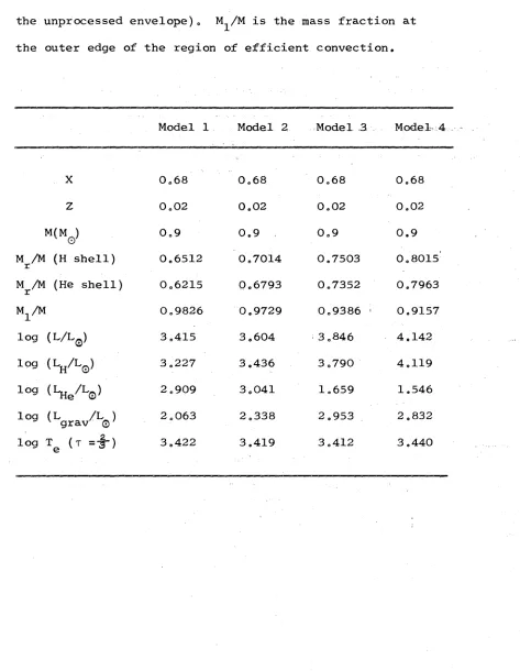
[image:43.553.67.540.198.808.2]TABLE 3.1
Parameters of the four 0.9 M models. The mass fractions
0
specified for the shells are those at which the nuclear energy generation rate is a maximum. X and Z are the mass fractions of hydrogen and elements heavier than helium (in the unprocessed envelope). M /M is the mass fraction at the outer edge of the region of efficient convection.
Model 1 Model 2 Model 3 Model 4
X 0.68
z
0.02M(Mq) 0.9
M r/M (H shell) 0.6512 M^/M (He shell) 0.6215
M 1/M 0.9826
log (L / Lq ) 3.415 iog (Lh/L0 ) 3.227
lo9
(Hie/L0>
2.909109 (Lgrav/L0 ) 2.063 log Te (t =-§-) 3.422
0.68 0.68 0.68
0.02 0.02 0.02
0.9 0.9 0.9
0.7014 0.7503 0.8015
0.6793 0.7352 0.7963
0.9729 0.9386 0.9157
3.604 3.846 4.142
3.436 3.790 4.119
3.041 1.659 1.546
2.338 2.953 2.832
Figure 3 „1
Variation of M /M and ß = P /P with radius in
r M gas
model 4« The cross on the M /M curve marks r
optical depth 2/3c
Figure 3 «2
LogCO
LogCp)
33
gradient is small due to the low opacity» (It should be noted that although much of this region is optically thin, the
diffusion approximation has been used») As the temperature increases, the H~ ion begins to contribute significantly to the opacity and the temperature gradient increases rapidly until the onset of efficient convection a t ^ 4 2 0 R offsets the effect on
G
the temperature gradient of further increases in the opacity« Although the region 420-490 is convectively unstable, almost no flux is carried convectively there»
Some properties of the convection zone are shown in Figures 3 «3 and 3,4» In the hydrogen and Hel ionization zones practically all the flux is carried convectively due to the high opacity and specific heat« Even though the convective efficiency parameter F >> 1, a strongly superadiabatic
gradient is needed to carry the energy flux» As the radius decreases, more of the flux is carried radiatively and the
super-adiabaticity of the temperature gradient is reduced„ The positions of the zones of ionization of H, Hel and Hell and the zone of H^ dissociation are shown clearly in Figure 3,5 by the variation of F^ and (per unit mass)« In
the interior regions, the radiation pressure causes C to become very large while at the same time reducing towards the value 4/3 characteristic of a photon gas»
Figure 3 „3
Variation of v/v u L /L and log ß with radius
ad c onv K
9
in model 4„ ß = — is a measure of the convective efficiency (see equation 2.23) c Scale limits of the variables are» 7/7 ,, 0-50; L /L, 0=1; log ft,
v v a d ’ ’ conv ’ ^ M ’ =5 to +5 e
Figure 3.4
Variation of v and P, , /P with radius in model 4. conv turb
Turbulent, pressure is not included in the model
V
co
n
v
C
k
m
/s
ec
)
conv
conv
P
tu
rb
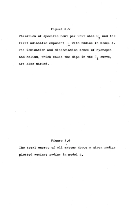
Figure 3.5
Variation of specific heat per unit mass and the first adiabatic exponent with radius in model 4. The ionization and dissociation zones of hydrogen and helium, which cause the dips in the curve, are also marked.
Figure 3.6
[image:49.553.55.531.85.804.2]E
n
e
rg
y
C
e
rg
s
)
o
•o
5
x
1
0
34
helium, together with the energy of radiation trapped within the envelope, is sufficient to make E positive throughout much of the envelopeo Hoyle (1956) and Paczynski and Ziolkowski (1968) pointed out this feature of red-giant envelopes and suggested that an efficient conversion of the envelope energy to kinetic energy could cause mass loss with velocities at infinity of a few tens of kilometers per second. However, as shown by Keeley (1970), Rose and Smith (1972) and in the present work, the behaviour of red-giant envelopes is highly non-
adiabatic with most of the ionization energy of hydrogen being radiated away rather than converted directly into kinetic and gravitational potential energy,
3.3 STRUCTURAL CHANGE OF THE STATIC MODELS WITH EVOLUTION
Figures 3,7 to 3 „10 compare the structure of the highest and lowest luminosity models (4 and 1 respectively). Other models lie between the extremes represented by these two models. As the burning shells consume mass at the interior of the
Figure 3 „7
Radius and ß = Pgas/P plotted against mass fraction for model 1 (dotted line) and model 4 (continuous line)o
Figure 3 e8
10
Figure 3 09
Log T plotted against: mass fraction for model 1 (dotted line) and model 4 (continuous line)„
Figure 3«10
35
of the envelope mass above the hydrogen ionization zone in the higher luminosity model and partly due to the increased
influence of radiation pressure0
Figure 3 „11 shows the position of the four models in the (log L/L , log T ) planec A first-giant branch evolutionary
0 e
track of Rood (1972) is shown for comparison» Tracks of first-giant branch stars of other recent authors (Eggleton 1968, Iben 1968, Demarque and Mengel 1971a, Faulkner and Cannon 1973) all terminate at log L/L < 3 „4, so that the four models considered
0 ~
here are more luminous than stars on the first-giant branch» The numbers on Figure 3 „11 are the mean periods in days of the groups of long-period variables studied by Osvalds and Risley (1961)» Smak7s (1964, 1966) calibrations of effective temperature and luminosity are used to place the groups in the
(log L/L , log T ) plane» The data refer to maximum light,
O e
but for reasonable (one magnitude) variations in bolometric luminosity, all groups except those of period 131 days and 324 days lie well above the first-giant branch at mean luminosity» Many long-period variables must therefore be asymptotic-giant branch stars» The periods of the long-period variables appear to increase as the effective temperature decreases and the radius increases»
36
to obtain loq T from the (R-I)„ coloursc The effective
temperatures of the models are cooler than EggenTs giant branch by 0 o06 in log T 0 However, the outer boundary conditions and the definition of effective temperature in the models are very crude, so that good agreement is not expected,, As an example of the uncertainty in log T , if the effective temperature is defined as the temperature at optical depth t = 1.0, rather than t =■§' , log increases by ~0.02„ In all models, the
2 4
value of log T satisfying L = 4rrcjr T is 0„01 to 0.02 hotter
2
than the value of log T at t .
It will take ^,3.3*10 years for an asymptotic-giant branch star to evolve from model 1 to model 4. The horizontal width of the region between the thin lines in Figure 3.11 is a rough estimate of the density of stars in the (log L/L , log T^) plane at. that luminosity (the width of the region does not represent a spread in log T ) . Assuming that the mass function is flat over the small range of initial stellar masses present
on the asymptotic-giant branch, and also assuming that mass loss has a negligible effect on giant branch evolution, the number n of stars per unit interval in log L/L on the giant
0 branch obeys the relation
x d log L/L d log L/L dMcoie
n ^ dt dM dt
core
where M increases monotonically with L/L . However, with
core 0
a constant mass fraction of hydrogen in the envelope
d M core
Figure 3 011
Position of the four models in the (log L/'L , log T )
0 e
CN CO
_ J |_ J
S’
— J
u->
9
to
CO
O C O CO
L
og
T
37
since most of the luminosity comes from the hydrogen burning shell and the mass between the hydrogen and helium burning shells does not vary rapidly with M r • Combining the above results gives
1
d L/LG
n ^ d Mcore
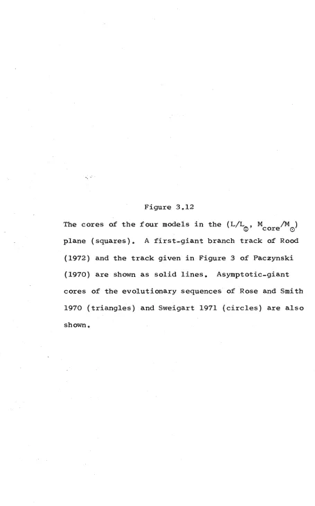
The four models are plotted in the (L/L , M /M ) plane in Figure 3 e12 together with the first-giant branch track of Rood (1972) and the asymptotic-giant branch tracks of Sweigart
(1971), Paczynski (1970) and Rose and Smith (1970), The width of the region between the thin lines in Figure 3.11 is a measure of n for the four models and for the first-giant branch track of Rood (1972), At log L/L ^>3.4, there are approximately
0
equal numbers of stars on the asymptotic- and first-giant branches (It is assumed here that the mass functions for
asymptotic- and first-giant branch stars are the same; however, 8
since ~2*10 years is spent in core helium burning between the two branches (Cannon 1970, Faulkner and Cannon 1972) there could be some difference in the mass function on the two branches, especially for more massive stars). At lower luminosities, the ratio of first- to asymptotic-giant branch stars will be
Figure 3 «12
The cores of the four models in the (L/L , M /M ) plane (squares)« A first-giant branch track of Rood
[image:61.553.32.487.61.790.2]15000
10000
5000
38
Since the luminosity, core-mass relations are reasonably independent of input parameters (total mass, Z) and
uncertainties in the physics of envelope convection, the relative number densities of first- and asymptotic-giant branch stars should be a function of the luminosity alone0
In those clusters in which asymptotic- and first-giant branch stars are photometrically separable, it may be possible to calibrate the luminosity from the relative number densities on
39
CHAPTER 4
ENVELOPE DYNAMICS OF FOUR 0.9 M ASYMPTOTIC-GIANT BRANCH STARS 0
In this chapter, the non-linear dynamical properties of the envelopes of four 0.9 M^ asymptotic-giant branch stars are investigated. Some effects of variations in the input physics are described and, finally, the results are discussed. The
luminosity and core mass of each envelope are obtained from a complete stellar model generated with program H2 and are
therefore consistent with the requirements of stellar evolution. Table 4.1 contains selected parameters of the four models.
4.1 DYNAMICAL BEHAVIOUR OF MODEL 1
( a) Results of the numerical calculations
Figure 4.1 shows the growth of the envelope kinetic
energy from a homologous perturbation with a surface velocity of 100 cm sec-1. Initially, the envelope pulsates in the
fundamental mode due to the form of the initial perturbation and because the time step (0.05 years) used in the early phases is
too long to allow the development of the first overtone. At low amplitudes, the oscillations grow exponentially with an e-folding time of 1.49 years and a period of 482 days. With the reduction in the size of the time step, a strong first overtone node
develops and continues to grow in amplitude until the rapid onset of equilibrium when the peak kinetic energy of the
42.4
Figure 4 01
40
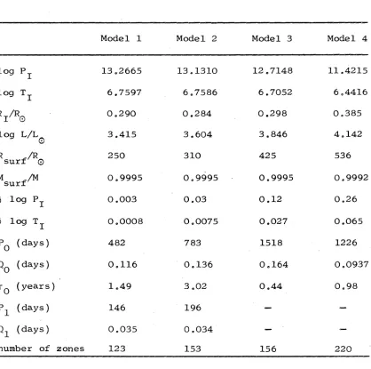
TABLE 4.1
Parameters of the dynamical models. Subscript I signifies that the quantity is evaluated at the inner boundary. 6 log P and
6 log Tj are the variations of log P and log T at the inner boundary during pulsation. ^ Su r f ^ i-s mass f a c t i o n at which the outer boundary conditions are applied and R ^ ^ is
the radius of the surface point. The growth rates of pulsation (t ) are obtained from the plots of kinetic energy against time.
Model 1 Model 2 Model 3 Model 4
log P I 13.2665 13.1310 12.7148 11.4215
log T T 6.7597 6.7586 6.7052 6.4416
R I/R0 0.290 0.284 0.298 0.385
log L/L
0 3.415 3.604 3.846 4.142
R V R
surf 0 250 310 425 536
M _/M
surf 0.9995 0.9995 0.9995 0.9992
5 log P 1 0.003 0.03 0.12 0.26
6 log T^ 0.0008 0.0075 0.027 0.065
PQ (days) 482 783 1518 1226
Q0 (days) 0.116 0.136 0.164 0.0937
t0 (years) 1.49 3 .02 0.44 0.98
P l (days) 146 196 — —
Q 1 (days) 0.035 0.034 — —
[image:67.553.77.495.302.717.2]Figure 4.2
o
TIME (TRS)
41
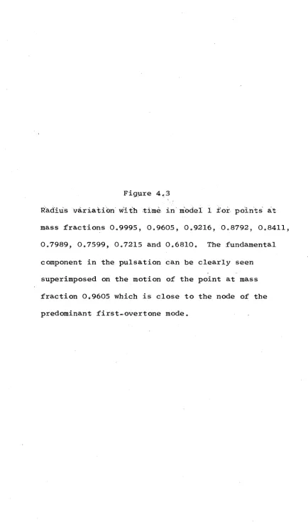
overtone is situated near the middle of the hydrogen ionization zone at mass fraction q = 0,96 (see Figure 4„7)„ At full amplitude, a fundamental component is still present in the pulsation as clearly seen in Figure 4.3, Modulation of the surface velocity and luminosity curves (Figure 4 „2) by the fundamental may contribute partially to the observation that mira variables do not repeat exactly from cycle to cycle»
A notable feature of the behaviour of this model is the slow contraction evident in Figure 4 «3» This is consistent with the fact that the average radiated luminosity is greater than the luminosity at the base of the envelope» Keeley (1970b) also found that pulsation of a static model caused it to contract»
In the present study, no large change in the period of the model resulted from structural re-arrangement over the period studied and the peak kinetic energy remained very constant throughout the contraction phase» On the other hand, Keeley (1970c) found that the period of his model decreased from 520 days to 300 days in 37 cycles» Model 1 may have undergone major structural change if the pulsation had been followed far enough but the relatively small amplitude (compared with Keeleycs fundamental pulsator) makes this unlikely»
Figure 4 C3
[image:71.553.47.481.58.793.2]n
/n
s
u
N
O
O
o
o
o
CVI
-on
o
t
o
-CO
- v w W V V V W
'wv^WWWvWWWWVW%v
I ~ ~ *• “ * *■ *■ *“ w‘ ^ *x,V ^ V ^ V W \ ^w\ A < Vw n aA A ^
6. 0
TIME CTRS)
I
Figure 4 04