Semiparametric Bayesian inference in multiple equation models

Bayesian Semiparametric Inference in Multiple Equation Models

Gary Koop Department of Economics

University of Leicester [email protected]

Dale J. Poirier Department of Economics University of California at Irvine

[email protected]

and

Justin Tobias Department of Economics University of California at Irvine

[email protected]

June 2003

KEYWORDS: nonparametric regression, nonparametric instrumental variables, SUR model, endogeneity, nonlinear simultaneous equations

1

Introduction

Despite the proliferation of theories for semiparametric and nonparametric regression, the use of these

techniques remains relatively rare in empirical practice. Increased computational difficulty and mathematical

sophistication, and perhaps most importantly, thecurse of dimensionality - wherein the rate of convergence

of the nonparametric regression estimator slows with the number of variables treated nonparametrically - all

seem to provide barriers which prevent the widespread use of nonparametric techniques.

The rapid increase in computing power and growth in nonparametric routines found in statistical software packages has helped to mitigate computational concerns. To combat the curse of dimensionality problem,

many researchers have adopted the use of thepartially linear orsemilinear regression model. This model,

though not fully nonparametric, provides a convenient generalization of the standard linear model which

is not as susceptible to the curse of dimensionality since only one, or perhaps a few, variables are treated

nonparametrically. Finally, some studies (e.g. Blundell and Duncan (1998), Yatchew (1999) and DiNardo

and Tobias (2001)) have tried to bridge the gap between theory and practice, and make these techniques accessible to applied researchers.

In this paper we continue in this tradition, and describe and implement simple and intuitive Bayesian methods

for semiparametric and nonparametric regression. Importantly, the methods we describe can be used in the

context of multiple equation models, thus generalizing the scope of models for which simple nonparametric

methods have been described. In our discussion, we focus primarily on the Seemingly Unrelated Regression (SUR) model. This model is of interest in and of itself, but is also of interest as the (possibly restricted)

reduced form of a semiparametric simultaneous equations model (or the structural form of a triangular

simultaneous equations model).

Before describing the contributions of this paper, it is useful to briefly outline the method we used in related

work (e.g. Koop and Poirier (2003a)) in the single equation partially linear regression model. This partially linear model divides the explanatory variables into a set which is treated parametrically,z, and a set which

is treated nonparametrically,x, and relates them to a dependent variabley as:

yi=z′

iβ+f(xi) +εi,

fori= 1, .., N where f() is an unknown function. Because of the curse of dimensionality,xi must be of low

dimension and is often a scalar (see Yatchew, 1998, for an excellent introduction to the partial linear model).

For most of this paper we will assumexi is a scalar, although this assumption is relaxed in Section 4.

In this model we assumed εi iid∼ N¡0, σ2¢ for i = 1, ..., N, and all explanatory variables were fixed or exogenous. Observations were ordered so thatx1< x2< ... < xN.Define y= (y1, ..., yN)′, Z= (z1,..., zN)′

previous equation could be written as:

y=W δ+ε.

Thus, the partially linear model can be written as the standard Normal linear regression model where the

unknown points on the nonparametric regression line are treated as unknown parameters. This regression

model is characterized by insufficient observations in that the number of explanatory variables is greater

thanN. However, Koop and Poirier (2003a) showed that, if a natural conjugate prior is used, the posterior

is still well-defined. In fact, we showed that the natural conjugate prior did not even have to be informative

in all dimensions and that prior information about the smoothness of the nonparametric regression line

was all that was required to ensure valid posterior inference. Thus, for the subjective Bayesian, prior information can be used to surmount the problem of insufficient observations. Furthermore, for the researcher

uncomfortable with subjective prior information, the required amount of prior information was quite small,

involving the selection of a single prior hyperparameter which we called η that governed the smoothness

of the nonparametric regression line. In Koop and Poirier (2003b), we went even further and showed how

(under weak conditions) empirical Bayesian methods could be used to estimateη from the data.

The advantages of remaining within the framework of the Normal linear regression model with a natural

conjugate prior are clear. This model is very well understood and standard textbook results for

estima-tion, model comparison and prediction are immediately available. Analytical results for posterior moments,

marginal likelihoods and predictives exist and, thus, there is no need for posterior simulation. This means

methods which search over many values for η (e.g. empirical Bayesian methods or cross-validation) can be

implemented at a low computational cost. Furthermore, as shown in our previous work, the partial lin-ear model can serve as a component in numerous other models which do involve posterior simulation (e.g.

semiparametric tobit and probit models or the partial linear model with the errors treated flexibly by using

mixtures of Normals). The ability to simplify the estimation of the nonparametric component in such a

complicated empirical exercise may provide the researcher a great computational benefit.

In this paper we take up the case of Bayesian semiparametric estimation in multiple equation models, and adopt a similar approach for smoothing the regression functions. In particular, we consider the estimation

of a semiparametric SUR model of the form:

yij =z′

ijβj+fj(xij) +εij, (1.1)

where yij is the ith _{observation (i= 1, .., N) on the endogenous variable in the j}th_{equation (j = 1, .., m),}

zij is a kj×1 vector of observations on the exogenous variables which enter linearly,fj(xij) is an unknown function which depends on a vector of exogenous variables,xij,andεij is the error term. For equations which

have nonparametric components,zij does not contain an intercept since the first point on a nonparametric

regression line plays the role of an intercept.

The approach we describe for the estimation of this model is simple and intuitive and, hopefully, will appeal

employ a prior which serves to smooth the nonparametric regression functions. It is important to recognize

that for the (parametric) seemingly unrelated regressions model (and the reduced form of the simultaneous

equations model), the natural conjugate prior suffers from well known criticisms (see Rothenberg, 1963,

or Dreze and Richard, 1983). On the basis of these, Dreze and Richard (1983, page 541) argue against using the natural conjugate prior (except for certain noninformative limiting cases not relevant for our class

of models). Their arguments carry even more force in the present semiparametric context since it can be

shown that the natural conjugate prior places some undesirable restrictions on the way smoothing is carried

out on nonparametric regression functions in different equations (i.e., the nonparametric component in each

equation is smoothed in the same way). Thus, in the present paper we do not adopt a natural conjugate

prior, but rather use an independent Normal-Wishart prior.

The basic ideas behind our approach are straightforward extensions of standard textbook Bayesian methods

for the SUR model (see, e.g., Koop (2003) pages 137-142). Thus, textbook results for estimation, model

comparison (including comparison of parametric to nonparametric models) and prediction are immediately

available. This, we argue, is an advantage relative to the relevant non-Bayesian literature (see, e.g., Pagan and

Ullah (1999) chapter 6) and to other, more complicated, Bayesian approaches to nonparametric seemingly unrelated regression such as Smith and Kohn (2000).

We illustrate the use of our methods by estimating a two-equation simultaneous equations model in parallel

with the development of our theory. This application takes data from the National Longitudinal Survey of

Youth (NLSY) and involves estimating the returns to schooling, job tenure, and ability for a cross-sectional

sample of white males. Our triangular simultaneous equations model has two equations, one for the (log) wage and the other for the quantity of schooling attained. After estimating standard parametric models that

have appeared in the literature, we first extend them to allow for nonparametric treatment of an exogenous

variable (weeks of tenure on the current job) in the wage equation (Case 1). Subsequently, we consider Case

2 where single explanatory variables enter nonparametrically in each equation. In this model we additionally

allow a measure of cognitive ability to enter the schooling equation nonparametrically. We complete our

empirical work with Case 3 by giving cognitive ability a nonparametric treatment in both the wage and

schooling equations (with tenure on the job also given a nonparametric treatment in the wage equation).

Our results reveal the practicality and usefulness of our approach. In some cases, our semiparametric

treatment yields results which are very similar to those from simple parametric nonlinear models (e.g.

quadratic). However, one advantage of a semiparametric approach is that a particular functional form such

as the quadratic does not have to be chosen, either in anad hoc fashion or through pre-testing. Furthermore,

in some cases our semiparametric approach yields empirical results that could not be easily obtained using standard parametric methods. In terms of our application, our results reveal the empirical importance of

controlling for nonlinearities in ability in both the wage and schooling equations when trying to estimate the

The outline of our paper is as follows. In the next section, we outline our basic semiparametric SUR model,

describe our data, and obtain parametric results and semiparametric results for a model where job tenure is

treated nonparametrically. In section 3, we describe the process of estimating a model with nonparametric

components in both equations, and estimate the model in Case 2. Finally, in section 4, we describe how to handle the estimation of additive models and provide estimation results for our most general Case 3. The

paper concludes with a summary in section 5.

2

Case 1: A Single Nonparametric Component in a Single

Equa-tion

We begin by considering a simplified version of (1.1) where a nonparametric component enters a single

equation (chosen to be the mth _{equation) and the explanatory variable which receives a nonparametric}

treatment,xim, is a scalar. In later sections, we consider cases where several equations have nonparametric

components each depending on a different explanatory variable (or variables).

We assume that the data is ordered so thatx1m< ... < xN m and define γi =fm(xim) fori= 1, .., N to be the unknown points on the nonparametric regression line in the mth_{equation. We also letγ = (γ}

1, .., γN)

′

andζi be theith_{row ofIN. With these definitions, we can write the model as:}

yi=Wiδ+εi, (2.1)

whereyi= (yi1, .., yim)

′

, εi= (εi1, .., εim)

′ , Wi=       z′

i1 0 . . . 0

0 z′

i2 . . . .

. . . .

. . 0 z′

i,m−1 0 0

0 . . 0 z′

im ζi      

andδ= (β′

1, .., β

′ m, γ

′

)′ is aK+N vector whereK=Pmj=1kj. For future reference, we define the partition

Wi=hW_i(1):W_i(2)iwhereW_i(1) is anm×(K+ 2) matrix andW_i(2) ism×(N−2). The likelihood for this

model is defined by assumingεiiid∼ N(0,Σ).

We define smoothness according to second differences of points on the nonparametric regression line. In light of this, it proves convenient to transform the model. Define the (N−2)×N second-differencing matrix as:

D=      

1 −2 1 . . . . 0

0 1 −2 1 0 . . 0

. . . .

. . . .

0 0 . . . 1 −2 1

      , (2.2)

so thatDγis the vector of second differences, ∆2_{γi. Prior information about smoothness of the nonparametric}

regression line will be expressed in terms ofRδ, where the (N−2)×(K+N) matrixR=£0(N−2)×K :D ¤

For future reference, we partitionR= [R1:R2] whereR1is an (N−2)×(K+ 2) matrix andR2is (N−2)×

(N−2) (i.e., the nonsingular matrixR2 isD with the first two columns deleted). Note that other degrees

of differencing can be handled by re-defining (2.2) as appropriate (see, e.g., Yatchew (1998) pages 695-698

or Koop and Poirier (2003a)).

Using standard transformations (see, e.g. Poirier (1995) pages 503-504), (2.1) can be written as:

yi=Vi(1)λ1+Vi(2)λ2+εi=Viλ+εi, (2.3)

where λ= (λ′

1, λ

′

2)

′

, λ1 = (β1′, .., β

′

m, γ1, γ2)

′

, λ2 =Dγ, Vi(1) =W

(1)

i −W

(2)

i R −1

2 R1 and Vi(2) =W

(2)

i R −1 2 .

Note thatλ2 is the vector of second differences of the points on the nonparametric regression line and it is

on this parameter vector that we place our smoothness prior.

We use an independent Normal-Wishart prior forλand Σ−1 _{which is a common choice for the parametric}

SUR model (see, e.g., Chib and Greenberg (1995) or (1996)). Thus,

λ∼N(λ, Vλ) (2.4)

and

Σ−1_∼

W¡V−1 Σ , ν

¢

, (2.5)

whereW(VΣ, ν) denotes the Wishart distribution (see, e.g., Poirier (1995) page 136).

Our empirical work is based on a Gibbs sampler involving p¡λ|y,Σ−1¢ _{and p}¡_Σ−1_{|y, λ}¢_{. Straightforward}

manipulations show these to be:

λ|y,Σ−1_∼N¡_{λ, V}

λ ¢

(2.6)

and

Σ−1_{|y, λ∼W}³_V−1 Σ , ν

´

, (2.7)

where

ν =ν+N, (2.8)

V−Σ1=

" VΣ+

N X

i=1

(yi−Viλ) (yi−Viλ)′ #−1

, (2.9)

Vλ= Ã

V−1

λ + N X i=1 V′ iΣ

−1_Vi

!−1

(2.10)

and

λ=Vλ Ã

V−1

λ λ+ N X

i=1

V′ iΣ

−1_y

!

. (2.11)

Of course, many values may be selected for the prior hyperparameters,λ, Vλ, V −1

Σ andν. Here we describe

a particular prior elicitation strategy that requires a minimal amount of subjective prior information. We

assume

Vλ= ·

V1 0

0 V (η) ¸

where V1 and V(η) are the prior covariance matrices for λ1 and λ2, respectively. We set V

−1

1 = 0, the

noninformative choice. Since λ2 = Dγ is the vector of second differences of points on the nonparametric

regression line,V(η) controls its degree of smoothness. We assumeV(η) depends on a scalar parameter,η.

As discussed in Koop and Poirier (2003a), several sensible forms forV(η) can be chosen. In this paper, we setV(η) =ηIN−2. We also setλ= 0K+N. Note that these assumptions imply we are noninformative about

λ1= (β′1, .., β

′

m, γ1, γ2)

′

, but have an informative prior for the remaining parameters which reflect the degree

of smoothness in the nonparametric regression line. Our information about this smoothness is of the form:

∆2_{γi∼N(0, η) fori= 3, .., N.}1

In this paper we adopt an empirical Bayesian approach whereη is chosen so as to maximize the marginal likelihood. However, it is worth noting that η could be treated either as a prior hyperparameter to be

selected by the researcher or as a parameter in a hierarchical prior. If the latter approach were adopted,η

could be integrated out of the posterior. Our empirical Bayesian approach is equivalent to this hierarchical

prior approach using a noninformative flat prior forη (and plugging in the posterior mode ofη instead of

integrating out this parameter).2

The results of Fernandez, Osiewalski and Steel (1997) imply that an informative prior is required for Σ−1

in order to ensure propriety of the posterior. However, in related work with a single equation model (see

Koop and Poirier (2003b)), we found that use of a proper, but relatively noninformative prior on a similar

nuisance parameter yielded sensible (and robust) results. Accordingly, we set ν = 10 in our application.

Using the properties of the Wishart distribution, we obtain the prior meanE(σ−1

ij ) =νV −1

Σij, whereσ −1

ij and

V−₁

Σij are theij

th_{elements of Σ}−1_andV−₁

Σ , respectively. To center the prior correctly, we calculate the OLS

estimate of Σ based on a parametric SUR model where all variables (including xim) enter linearly. We set

νV−1

Σ equal to the inverse of this OLS estimate.

In order to compare models or estimate/selectηin our empirical Bayesian approach, the marginal likelihood

(for a given value ofη) is required. No analytical expression for this exists. However, we can estimate the

marginal likelihood using Gibbs sampler output and the Savage-Dickey density ratio (see, e.g., Verdinelli and

Wasserman (1995)). DefineM1to be the semiparametric SUR model given in (2.3) with prior given by (2.4)

and (2.5) and a particular value forη selected. DefineM2to beM1with the restrictionλ2= 0N−2imposed

(with the same prior forλ1 and Σ−1). Using the Savage-Dickey density ratio, the Bayes factor comparing

M1 toM2 can be written as:

BF(η) = p(λ2= 0|M1) p(λ2= 0|y, M1)

, (2.13)

where the numerator and denominator are the prior and posterior, respectively, ofλ2 in the semiparametric

SUR model evaluated at the pointλ2= 0N−2. This Bayes factor may be of interest in and of itself since it

1

This approach to prior elicitation does not include any information in xim other than order information (i.e. data is

ordered so thatx1m< ... < xN m). If desired, the researcher could includeximby eliciting a prior, e.g., of the form ∆2γi∼

N 0, η∆2

xim

.

2

compares the semiparametric SUR model to a sensible parametric alternative.3 _{However, it can also be used}

in an empirical Bayesian analysis to selectη. That is, since η does not enter the prior for M2, BF(η) will

be proportional to the marginal likelihood for the semiparametric SUR model for a given value ofη. The

empirical Bayes estimate ofη can be implemented by running the Gibbs sampler for a grid of values forη and choosing the value which maximizesBF(η). Alternative methods for selectingηinclude cross-validation

or extensions of the reference prior approach discussed in van der Linde (2000).

Note that BF(η) can be calculated in the Gibbs sampler in a straightforward manner. The quantity

p(λ2= 0|M1) can be directly evaluated using the Normal prior given in (2.4), whilep(λ2= 0|y, M1) can be

evaluated in the Gibbs sampler in the same way as any posterior function of interest. That is, if we define

b

p(λ2= 0|y, M1) =

1 S

S X

s=1

p³λ2= 0|y,Σ(s)

´ ,

where Σ(s) _{for s = 1, .., S denotes draws from the Gibbs sampler (after discarding initial burn-in draws),}

then

b

p(λ2= 0|y, M1)→p(λ2= 0|y, M1)

asS→ ∞. Note that the posterior conditionalp¡λ2= 0|y,Σ(s)

¢

is simple to evaluate since it is Normal (see

equation 2.6).

This semiparametric SUR model can be used as a restricted reduced form of a semiparametric simultaneous

equations model and, thus, the methods described above allow for Bayesian inference in the latter model.

That is, our Gibbs sampler provides us with draws from the posterior of the reduced form parameters. Provided the model is identified, the structural form parameters will be a transformation of the reduced

form parameters and the draws of the latter can be transformed into draws of the former. The triangular

structure of the model in our application means we do not have to adopt such an approach. However, it is

useful to note that our approach can be used with more general simultaneous equations models.

Before introducing our application, we briefly discuss related (parametric) work on simultaneous equations models. The literature on Bayesian analysis of simultaneous equations models is voluminous. Dreze and

Richard (1983) surveys the literature through the early 1980s, while Kleibergen (1997), Kleibergen and van

Dijk (1998) and Kleibergen and Zivot (2003) are recent references. The more recent literature focusses on

issues of identification and prior elicitation which are of little relevance for our work. For instance, some of

this recent work discusses problems with the use of noninformative priors at points in the parameter space

which imply non-identification (and show how noninformative priors based on Jeffreys’ principle overcome

these problems). However, these problems are less empirically relevant if the posterior is located in regions of the parameter space away from the point of non-identification or if informative priors are used. Furthermore,

parameters in the reduced form model do not suffer from these problems. Hence, we feel some of the problems

3

Note thatλ2= 0 implies the nonparametric regression line is perfectly smooth (i.e. is a straight line). Thus,M2 is nearly

equivalent to a SUR model with an intercept andxim entering linearly. It is not exactly equivalent since we are only using

discussed in, e.g., Kleibergen and van Dijk (1998) are not critical for our work. In some sense, these problems

all involve prior elicitation and, with moderately large data sets, data information should predominate.4 _In

practice, we argue that our approach should be a sensible one for practitioners and that the advantage of

being semiparametric outweighs any costs associated with not eliciting priors directly off of structural form parameters.

2.1

The Parametric SEM

In this section we provide an empirical example to illustrate how our techniques can be applied in practice.

Our specific example, though primarily illustrative in nature, simultaneously addresses several topics of

considerable interest in labor economics. Specifically, we will introduce and estimate a two equation structural

simultaneous equations model and permit various nonparametric specifications within this system. The two

endogenous variables in our system will be the log hourly wage received by individuals in the labor force and

the quantity of schooling attained by those individuals. While many studies have recognized the potential endogeneity of schooling in standard log wage equations (see Card (1999) for a review of recent instrumental

variable studies on this issue), these studies do not typically estimate the full underlying structural model,

and have not allowed for nonparametric specifications within these systems.

To fix ideas, the fully parametric version of our model may be written as:

si=zC′

i αS1 +ziS′α2S+uSi

wi=α0+ρsi+zC′i αW1 +zW

′

i αW2 + +uWi ,

(2.14)

with _·

us i uw

i ¸

iid

∼N ·µ

0 0

¶ ,

µ

σ2s σsw σsw σ2w

¶¸

≡N(0,Σ).

In the above equationzC

i is akC−vector of exogenous variables common to both equations,z S

i is akS−vector of exogenous variables which enter only the schooling equation (i.e., these are the instruments) andzW

i is

a kW−vector of exogenous variables which enter only the wage equation. The parameters in (2.14) are structural, withρbeing the returns to schooling parameter that is often of central interest. The triangular

structure of (2.14) implies that the Jacobian is unity, so that we can directly estimate the structural form

using the methods we have developed in the previous section for the semiparametric SUR model.

In our empirical work we generalize this fully parametric structural model by permitting nonparametric

specifications for a few variables in this system. We divide our empirical analysis into three cases, with each case adding a new nonparametric component. In Case 1 we add a nonparametric specification to our wage

equation and treat tenure on the job nonparametrically. Several studies in labor economics (e.g. Altonji and

Shakotko (1987), Topel (1991), Light and McGarry (1998) and Bratsberg and Terrell (1998)) have addressed

4

the issue of separating the effects of on-the-job tenure and total labor market experience, with all of these

studies specifying parametric (typically quadratic) specifications for each of these variables. In Case 1, we

include a linear experience term and a nonparametric tenure term to flexibly investigate the shape of the

relationship between job tenure and labor market experience. In Case 2, we add a nonparametric component to the schooling equation and treat the “ability” variable nonparametrically. In this analysis, “ability”

refers to measured cognitive ability, and is proxied by a (continuous) test score that is available in our data

set. Finally, in Case 3 we also treat this ability variable nonparametrically in our wage equation.5 _Before

discussing our models and results in more detail, we first describe the data used in this analysis.

2.2

The Data

To estimate our models we take data from the National Longitudinal Survey of Youth (NLSY). The NLSY is a widely-used panel study containing a wealth of demographic information regarding a young cohort of

U.S. men and women. Survey information from the NLSY begins in 1979, at which point the respondents

range in age from 14 and 22. Sample participants are re-interviewed annually until 1994, and then additional

biennial interviews were conducted.

To illustrate the use of our methods and remain consistent with the models described above, we abstract

from the panel aspect of the NLSY and focus only on cross-sectional wage outcomes in 1992. We choose this year since key variables of interest are directly available in that year, and since the NLSY participants range

in age from 27-35 in 1992 and thus are likely to have completed their education and possess a reasonable

degree of labor market experience. In keeping with this literature and to abstract from selection issues into

employment, we also focus exclusively on the outcomes of white males in the NLSY.

Key to identification of this simultaneous equations model is the availability of an instrument or exclusion restriction. In the context of our application we need to find some variable that affects the quantity of

schooling attained, yet has no direct structural effect on wages given the other controls we employ. To this

end, we depart from the usual supply-side IV literature (e.g. Card (1999)) and use the quantity of schooling

attained by the respondent’s oldest sibling (SIBED) as our instrument.6 _{The argument behind the use of this}

instrument is that sibling’s education should be strongly correlated with one’s own schooling. This correlation

could arise, for example, from unobserved family attitudes toward the importance of education, or credit constraints faced by the family. However, we argue that the only channel through which sibling’s education

affects one’s own wages is an indirect one (through the quantity of schooling attained), since conditioned

on the schooling of the respondent himself and added controls for family background, the education of the

5

In related work, Cawley, Heckman and Vytlacil (1999) argue that ability enters the wage equation nonlinearly. Blackburn and Neumark (1995), Heckman and Vytlacil (2001) and Tobias (2003) examine if returns to schooling vary with ability. The latter two of these studies obtain results by allowing for flexible specifications of the relationship between ability and log wages.

6

sibling should play no structural role in the wage equation.7

To estimate our models of interest we also need to obtain information about the actual labor market

experi-ence of the individual as well as his tenure on the current job in 1992. The job tenure (TENURE) variable is readily available, as the NLSY directly provides information on the total tenure (in weeks) with the current

employer. As for total labor market experience, in each year of the survey the NLSY constructs the total

number of weeks worked since the previous interview date. Since information for some weeks is occasionally

missing, the NLSY also has a companion question that provides the percentage of weeks unaccounted in

each year in the construction of this weeks of work variable. As such, we confine our attention to only those

individuals whose weeks are fully accounted for in each year, and aggregate these experience variables across years to obtain our measure of total labor market experience (EXPERIENCE).8

In both the schooling and wage equations, we include the respondent’s Armed Forces Qualifying Test (AFQT)

score which is standardized by age (denoted ABILITY), highest grade completed by the respondent’s mother

(MOMED) and father (DADED), and a dummy variable equal to 1 if the respondent lives with both of his

parents at age 14 (NON-BROKEN). In the wage equation, we also include weeks of actual labor market experience (EXPERIENCE), weeks of tenure at the current job (TENURE), a dummy for residence in an

urban area (URBAN), and a continuous measure of the local unemployment rate (UNEMP). When measured

in weeks, both EXPERIENCE and TENURE can be regarded as approximately continuous variables. Our

sample restrictions are quite strict, and produce a clean, but relatively small data set. To summarize: we

limit our focus to white men in 1992 with older siblings at least 24 years of age in the base year of the survey

and with complete information on the remaining variables. In addition, we exclude several extra observations for those individuals who report to be currently enrolled in school in 1992, who are in the military subsample,

whose hourly wage exceeds $100 or is less than $1 per hour or who report to have completed less than 9

years of schooling. This leaves us with a total of N = 303 observations, for which an exact finite-sample

Bayesian analysis seems particularly useful.

2.3

Parametric Results

Before presenting results from our semiparametric models, we briefly present results using two standard

parametric approaches. The first of these simply estimates the structural wage equation ignoring potential

endogeneity problems. In this model we include an intercept, linear terms in the explanatory variables

described above and a quadratic in TENURE.9 We estimate this model using a fully noninformative prior

7

Simple regression analyses that included sibling’s education along with the other controls found no significant role for SIBED in the log wage equation.

8

This definition is not without controversy, with many researchers (e.g. Wolpin (1992) and Bratsberg and Terrell (1998)) only considering labor market experience after the completion of high school (or looking at only “terminal” high school graduates). Light (1998) investigates this issue and finds sensitivity of results to the definition of the career starting point. In this analysis, we do not make a distinction between pre-high school and post-high school labor market experience.

9

so that our results can be interpreted as the Bayesian counterpart to using OLS techniques on the structural

wage equation, for now, ignoring potential endogeneity issues. The second of our parametric models estimates

the two equation structural model in (2.14). The prior for all of the regression coefficients is noninformative.

For Σ−1_{we use the same prior as for the semiparametric model (see the discussion of the prior for Case 1).}

Table 1 presents empirical results for the coefficients in these parametric models. The results are mostly

sensible. The coefficient on our instrument SIBED is positive, as expected, with a posterior mean more

than twice its posterior standard deviation.10 _{We also note that results from single equation estimation of}

the wage equation (which ignores the endogeneity problem) are quite similar to results obtained the two

equation system. For instance, in both cases the point estimate of the return to schooling parameter is roughly 8 percent, and the results for the remaining coefficients are highly similar. The main differences in

results occur with the posterior standard deviations for the coefficients on the highly correlated variables

SCHOOL and ABILITY, which are much larger in the two equation model. This reduction in precision

can be explained by the fact that although the point estimate of the correlation between the errors in the

two equations is not far from zero (i.e., it is 0.054), it is relatively imprecisely estimated with this modest

sample size (i.e., the posterior standard deviation of this coefficient is 0.252). Thus, although the point estimate suggests that endogeneity is not a problem in this data set (and, hence, point estimates of key

parameters do not change much when we control for endogeneity), the posterior for Σ is quite dispersed and

allocates appreciable probability to regions of the parameter space where endogeneity is a problem. Given

this uncertainty regarding the empirical importance of endogeneity, the standard errors associated with these

parameters tend to increase relative to the model which ignores endogeneity concerns.

The finding that appreciable posterior probability is allocated to regions where the correlation between

the errors in the two equations is near zero or small in magnitude is consistent with some of the other

empirical work in this literature.11 _{That is, it has often been either assumed or more formally argued that}

after controlling for a rich set of explanatory variables, endogeneity problems are likely to be mitigated.

Our analysis lends some additional credence to this claim, as we “test down” from a structural model that

permits endogeneity, and find little evidence that endogeneity is a serious empirical issue for this model.

As we show in later sections, however, we find evidence against this basic parametric model, and in our generalized model specifications, there is some indication of a need to control for endogeneity of schooling.

10

In fact, we find a “significant” role for this instrument in all of our model specifications.

11

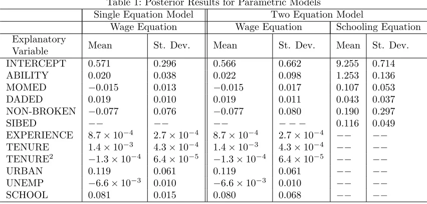
Table 1: Posterior Results for Parametric Models

Single Equation Model Two Equation Model

Wage Equation Wage Equation Schooling Equation

Explanatory

Variable Mean St. Dev. Mean St. Dev. Mean St. Dev.

INTERCEPT 0.571 0.296 0.566 0.662 9.255 0.714

ABILITY 0.020 0.038 0.022 0.098 1.253 0.136

MOMED −0.015 0.013 −0.015 0.017 0.107 0.053

DADED 0.019 0.010 0.019 0.011 0.043 0.037

NON-BROKEN −0.077 0.076 −0.077 0.080 0.190 0.297

SIBED −− −− −− − − − 0.116 0.049

EXPERIENCE 8.7×10−4 _2.7×10−4 _8.7×10−4 _2.7×10−4 _{−− −−}

TENURE 1.4×10−3 _4.3×10−4 _1.4×10−3 _4.3×10−4 _{−− −−}

TENURE2 _−1.3×10−4 _6.4×10−5 _−1.3×10−4 _6.4×10−5 _{−− −−}

URBAN 0.119 0.061 0.119 0.061 −− −−

UNEMP −6.6×10−3 _{0.010 −6.6×10}−3 _{0.010 −− −−}

SCHOOL 0.081 0.015 0.080 0.068 −− −−

2.4

Case 1: Application

In this model, we elaborate (2.14), and allow the variable TENURE to enter the log wage equation

nonpara-metrically. Formally, we specify:

si=zC′

i αS1 +ziS′αS2 +uSi

wi=ρsi+zC′

i αW1 +ziW′α2W +f(xi) +uWi ,

(2.15)

where xi denotes the number of weeks of work on the current job (TENURE) and ziW no longer contains

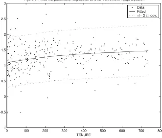
TENURE. In our analysis, we set η = 5×10−9_{, which is the empirical Bayes estimate that maximizes}

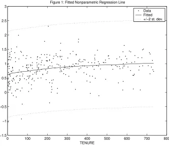
the marginal likelihood (see Figure 2). Figure 1 plots the fitted nonparametric regression line against the

data (after removing the effect of the other explanatory variables). That is, Figure 1 plots the posterior mean of the nonparametric regression line (and +/- two standard deviation bands) and the “data” points

have coordinates xi and wi−ρsi−zC′

i αW1 −zW

′

i αW2 for i = 1, .., N where all parameters are evaluated

at their posterior means. Figure 2 plots the log of the Bayes factor in favor of the semiparametric model

over the parametric model with a linear TENURE term across alternate choices of η (see equation 2.13).

It can be seen that the maximum of the log Bayes factor is 0.026. Thus, there is only slight support for

our semiparametric model over the parametric model with a linear tenure term. Note that as η → 0, the nonparametric and linear models become equivalent and the log Bayes factor is zero. The value of η that

maximizes the marginal likelihood is quite close to this case. However, Figure 2 does indicate an interior

maximum, so a model with slight nonlinearities that suggest a concave tenure profile is preferred over the

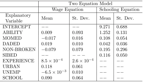
Table 2: Posterior Results for the Case 1 Semiparametric Model Two Equation Model

Wage Equation Schooling Equation Explanatory

Variable Mean St. Dev. Mean St. Dev.

INTERCEPT −− −− 9.271 0.688

ABILITY 0.009 0.093 1.252 0.131

MOMED −0.017 0.016 0.108 0.054

DADED 0.019 0.010 0.042 0.036

NON-BROKEN −0.079 0.079 0.195 0.296

SIBED −− − − − 0.116 0.050

EXPERIENCE 8.5×10−4 _2.6×10−4 _{−− −−}

URBAN 0.118 0.061 −− −−

UNEMP −6.5×10−3 _{0.010 −− −−}

SCHOOL 0.090 0.064 −− −−

The results in Table 2 are very similar to the two equation results in Table 1 which differ in that TENURE

and TENURE2_{are included parametrically. The point estimate of returns to schooling, at 9.0%, is slightly}

higher than with the parametric models. However, relative to its posterior standard deviation this difference

is minor. The posterior mean of the correlation between the errors in the two equations is also very similar

to that of the parametric model (i.e., its posterior mean is 0.031 and standard deviation is 0.231). Overall,

we find our nonparametric function of TENURE to be playing a nearly identical role to the quadratic

specification of this variable in the parametric model.

A comparison between a parametric SUR with TENURE entering quadratically to the semiparametric SUR

can be done by first calculating the Bayes factor in favor of the quadratic SUR model of Table 1 against

the parametric SUR with TENURE entering linearly (call this Bayes factor BF∗

to distinguish it from

BF(η) defined in equation 2.13).12 _{That is,BF(η) compares the semiparametric SUR against a linear SUR}

(subject to the qualification of footnote 3), and thus the two Bayes factors BF∗

and Bf(η) will each be

comparing a nonlinear (either quadratic or nonparametric) specification to the linear one. However, Bayes factor calculation requires an informative prior over parameters which are not common to both models.

Thus, to calculateBF∗

we require an informative prior for the coefficient on TENURE2 _{which we choose to}

beN¡0, vq ¢

. With this prior,BF∗

can be calculated using the Savage-Dickey density ratio with the strategy

discussed above (see the discussion around equation 2.13). The elicitation of prior hyperparameters such as

vq can be difficult (which is a further motivation for our empirical Bayesian analysis of a semiparametric

model). In our application, values of vq greater that 10

−10 _{indicate support for the linear model (i.e.,}

BF∗

<1). This apparently informative choice of prior variance is actually not that informative relative to

the data information (note that the posterior standard deviation of this coefficient in Table 1 is 6.4×10−5_).

Forvq<10

−10_{, the quadratic model is supported (i.e.,BF}∗

>1). However, there is no value forvqfor which

the quadratic model receives overwhelming support. The maximum value forBF∗

is 2.77 which occurs when

12

0 100 200 300 400 500 600 700 800 −1.5

−1 −0.5 0 0.5 1 1.5 2 2.5 3

Figure 1: Fitted Nonparametric Regression Line

TENURE

Data Fitted +/−2 st. dev.

vq = 10 −12_.13

This prior sensitivity analysis for the quadratic model can be interpreted in various ways, but regardless of how it is interpreted it is clear that the performance of the semiparametric and quadratic models (as

measured by their marginal likelihoods) is similar. This is despite the fact that there is a strong support

for parsimony implicit in Bayes factors. In the quadratic parametric model, deviations from linearity are

modelled by adding a single extra parameter, but in our semiparametric model deviations from linearity

are modelled by adding N−2 extra parameters. Hence, we would expect our semiparametric model to be penalized relative to the quadratic model. In any empirical exercise, if the researcher knows the correct functional form of the nonlinearity then it is best to work with the parametric model which captures this

functional form. However, the advantage of the nonparametric approach is that the data can be used to

decide the (here roughly quadratic) functional form. With the parametric model, preliminary estimation

and pretesting were required to select “down” to the quadratic functional form. Hence, in our case it is not

advisable to compare the quadratic model to the semiparametric model using a Bayes factor which ignores

the model selection issues involved with the quadratic model.

13

0 0.1 0.2 0.3 0.4 0.5 0.6 0.7 0.8 0.9 1

x 10−8 −0.03

−0.02 −0.01 0 0.01 0.02 0.03

Figure 2: Log of Bayes Factor in Favor of Semiparametric Model

eta

3

Case 2: A Single Nonparametric Component in Several

Equa-tions

In this section, we consider the more general semiparametric SUR model given in (1.1) where a nonparametric

component potentially exists in every equation. That is, γij =fj(xij) for j = 1, .., m is the ith _{point on}

the nonparametric regression line in the jth equation. We maintain the assumption that xij is a scalar.

Simple Bayesian methods for this model can be developed similarly to those developed for Case 1. We

adopt the same strategy of treating unknown points on the nonparametric regression lines as unknown parameters and, hence, augment each equation withN new explanatory variables (as in equation 2.1). We

then use a smoothness prior on each nonparametric regression line (analogous to equations 2.4 and 2.12).

The resulting posterior can be handled using a Gibbs sampler (analogous to equations 2.6 and 2.7). Note,

however, that we expressed our smoothness prior in terms of the second-differencing matrixDgiven in (2.2).

This prior required the data to be ordered so thatx1m< ... < xN m. However, unless each equation has its

nonparametric component depending on the same explanatory variable (i.e.,xij =xim forj= 1, .., m−1), the data in thejth_{equation (forj= 1, .., m−1) will not be ordered in such a way that a smoothness prior can} be expressed in terms ofD. However, this can be corrected for by redefining the explanatory variables. This

requires some new, somewhat messy, notation. Unless otherwise noted, all other assumptions and notation

are as for Case 1. For future reference, defineγj = (γ1j, ..., γN j)

In Case 1, the inclusion of the nonparametric component implied that the identity matrix,IN, was included

as a matrix of explanatory variables (see equation 2.1 and the surrounding definitions). Here we defineI∗ j

which is the identity matrix with columns rearranged to correspond to the ordering of the data in the jth

equation forj= 1, .., m. Thus, sincex1m< ... < xN m,I ∗

mis simplyIN, but the other equations potentially involving a reordering of the columns ofIN. Also defineζij to be the ith_{row ofI}∗

j.

A concrete example of how this works might help. Suppose we haveN = 5 observations and the explanatory

variables treated nonparametrically in the m = 2 equations have values in the columns of the following

matrix: _      3 1 4 2 1 3 2 4 5 5       .

The data has been ordered so that the second explanatory variable is in ascending order, x12 < ... < x52

and, hence, the Case 1 smoothness prior can be directly applied in the second equation. However, the first explanatory variable is not in ascending order. However, we can reorder the columns of the identity matrix

as I∗ 1 =      

0 0 1 0 0

0 0 0 1 0

1 0 0 0 0

0 1 0 0 0

0 0 0 0 1

      .

It can be seen that withI∗

1 used to define the nonparametric explanatory variables for the first equation,γ11

is the first point on the nonparametric regression line, γ21 is the second point, etc.. Thus, the smoothness

prior can be expressed as restrictingDγ1.

In Case 1, we noted that the smoothness prior was only anN−2 dimensional distribution for theN points on each nonparametric regression line. Implicitly, this prior did not provide any information about the

initial conditions (i.e., what we calledγ1 andγ2in Case 1), but only the second differences of points on the

nonparametric regression line,γi−2γi−1+γi−2. For the initial conditions, we used a noninformative prior.

This need to separate out initial conditions necessitates the introduction of more notation. Define the 2×1 vector of initial conditions in every equation asγ0

j forj= 1, .., m. Letγ ∗

j beγj with these first two elements deleted. Similarly, letI∗∗

j beI ∗

j with its first two columns deleted andI ∗∗∗

j be the two deleted columns. Also

define ζ∗

ij to beζij with the first two elements deleted and ζij0 be the two deleted elements. Analogously, partitionD= [D∗∗

D∗

] whereD∗∗

contains the first two columns ofD.

With all these definitions, we can write the Case 2 semiparametric SUR as (2.1) with

Wi=       z′

i1 ζi01 0 . . . 0 ζ

∗

i1 0 . . 0

0 0 z′

i2 ζi02 . . . 0 ζ

∗

i2 . . .

. . . .

. . . . 0 z′

i,m−1 ζi,m−0 1 0 0 . . 0 ζ

∗

i,m−1 0

0 . . . 0 z′

im ζim0 0 . . . ζ

whereδ=¡β′

1, γ0

′

1, .., β

′ m, γ0

′ m, γ

∗′

1, .., γ

∗′ m ¢′

is a K+mN vector of coefficients.

Prior information about smoothness of the nonparametric regression lines will be expressed in terms ofRδ,

where them(N−2)×(K+mN) matrix Ris given by

R=      

0 D∗∗

0 . . . . 0 D∗

0 . . 0

. 0 D∗∗

. . . . 0 D∗

. . .

. . . .

. . . D∗∗

0 0 . . . D∗

0

. . . 0 0 D∗∗

0 . . 0 D∗

      . (3.2)

The remainder of the derivations are essentially the same as for Case 1. Define the partitions Wi == h

W_i(1):W_i(2)iwhereW_i(1) is anm×(K+ 2m) matrix andW_i(2) ism×m(N−2) andR= [R1:R2] where

R1 is anm(N−2)×(K+ 2m) matrix and R2 ism(N−2)×m(N−2). Transform the model as:

yi=Vi(1)λ1+Vi(2)λ2+εi=Viλ+εi, (3.3)

where λ= (λ′

1, λ

′

2)

′

, λ1=¡β′1, γ0

′

1, .., β

′ m, γ0

′ m ¢′

,λ2=Rδ=£(Dγ1)

′

, ..,(Dγm)′¤′,V_i(1) =W_i(1)−W_i(2)R−1 2 R1

andV_i(2)=W_i(2)R−1 2 .

This model is now in the same form as Case 1. Given an independent Normal-Wishart prior as in (2.4) and

(2.5), posterior analysis can be carried out using the Gibbs sampler described in (2.6) through (2.11). As in

Case 1, we use a noninformative prior forλ1. The prior for Σ−1uses the same hyperparameter values as in

Case 1. The smoothness prior relates toλ2 and, for this, we extend the prior of Case 1 (see equation 2.12)

to be:

V(η1, .., ηm) =

     

η1IN−2 0 . . 0

0 η1IN−2 0 . .

. 0 . . .

. . . . 0

0 . . 0 ηmIN−2

      . (3.4)

Thus, the nonparametric component of each equation can be smoothed to a different degree. An empirical Bayesian analysis can be carried out as described above (see equation 2.13 and surrounding discussion). The

computational demands of empirical Bayes in this general case can be quite substantial since a search over

mdimensions of the smoothing parameter vector must be carried out.

3.1

Case 2: Application

For Case 2, we extend the Case 1 model to allow for an exogenous variable in the schooling equation to receive a nonparametric treatment. The model we consider here is:

si=zC′

i αS1 +zS

′

i αS2 +f1(xi1) +uSi

wi =ρsi+ziC′α W

1 +ziW′α W

2 +f2(xi2) +uWi

, (3.5)

where all definitions are as in (2.15) except that xi1 is ABILITY and xi2 is TENURE and ziC no longer

smooth the nonparametric regression lines in the two equations. This leads us to set η1 = 5×10−6 and

η2= 10−11.

Table 3 presents posterior results for the parametric coefficients in this semiparametric model. As found in our previous results, the correlation between the errors in the two equations has a point estimate near to,

but now farther away from zero (i.e., its posterior mean is 0.102) and remains very imprecisely estimated

(i.e., its posterior standard deviation is 0.142). Thus, we have more evidence that endogeneity is an issue in

model specification. Other results can be seen to be similar as for Case 1.

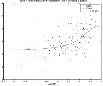
Interestingly, this analysis finds rather strong evidence of nonlinearities in the relationship between ability and schooling. The log of the Bayes factor of our semiparametric model against the linear-in-schooling

model is 4.645, which indicates substantially more support for departures from linearity than was found

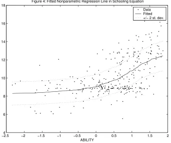
in Case 1. Figures 3 and 4 plot the posterior means of the two nonparametric regression lines against the

data (after controlling for parametric explanatory variables). That is, the “data” points in Figure 3 plot

TENURE against wi−ρsi−zC′ i α

W

1 −zW

′ i α

W

2 for i = 1, .., N where all parameters are evaluated at their

posterior means. The comparable points in Figure 4 plot ABILITY againstsi−zC′

i αS1 −ziS′αS2 (evaluated

at the posterior means for αS

1 and αS2). Figure 3 looks very similar to Figure 1 and indicates some slight

nonlinearities that appear quadratic. Figure 4 indicates more interesting (and more precisely estimated)

nonlinear effects that would not be captured by simple parametric methods (e.g. including ABILITY in

a quadratic manner).14 _{Specifically, the graph suggests that marginal increments in ability for low ability}

individuals does little to increase the quantity of schooling attained (i.e.,the graph is quite flat to the left

of zero). However, for those individuals above the mean of the ability distribution, marginal increments in ability significantly increase the likelihood of acquiring more schooling. The fact that ability is a strong

predictor of schooling has been well-documented (e.g. Heckman and Vytlacil (2000)), and here we add to

this result by finding that it is relatively high ability individuals whose schooling choices are most affected

by changes in ability.

It is also of interest to note that results for the returns for schooling parameter are slightly lower than what

we have seen in either the parametric model or Case 1, with a posterior mean of 0.058 and posterior standard deviation of 0.038. We will now try to reconcile why this reduction has taken place. Our semiparametric

estimation results found strong evidence of a nonlinear (and convex) relationship between ability and the

quantity of schooling attained. To illustrate how this convex relationship may lead to a reduction of the

schooling coefficient, let’s suppose for the sake of simplicity that the actual relationship between schooling and

ability is quadratic, with a positive coefficient on the squared term. Since the correlation between the errors

of the structural equations of Case 2 is non-zero (or at least most of the posterior mass is concentrated away from zero), this implies that the conditional mean of wages given schooling (i.e.,the “reduced form” wage

equation from our structural model), will now contain the nonlinear ability term that enters the education

14

If we add ABILITY2

equation. This nonlinear term was, of course, not present in the conditional mean of Case 1 since that model

only contained a linear ability term. So, we can regard the differences between the conditional means of

Case 2 and Case 1 as essentially an omitted variable problem - in Case 2 we have an added quadratic ability

term that is positively correlated with education (see Figure 4) and also positively correlated with log wages (we provide evidence of this in the next section). Using standard omitted variable bias formulas, we would

thus predict a reduction in the “reduced form” schooling coefficient upon controlling for this nonlinearity in

ability. This result has potentially significant implications for this literature, as it suggests the importance

of controlling for potential nonlinearities in ability (in both the schooling or wage equations) in order to

extract accurate estimates of the return to education. Despite this result, it is also important to recognize

that the shift in the posterior of this key parameter is small relative to its posterior standard deviation.

Table 3: Posterior Results for the Case 2 Semiparametric Model Wage Equation Schooling Equation Explanatory

Variable Mean St. Dev. Mean St. Dev.

SIBED −− −− 0.087 0.047

ABILITY 0.051 0.061 −− −−

MOMED −0.012 0.015 0.123 0.052

DADED 0.021 0.010 0.050 0.035

NON-BROKEN −0.068 0.077 0.045 0.287

EXPERIENCE 8.0×10−4 _2.7×10−4 _{−− −−}

URBAN 0.124 0.062 −− −−

UNEMP −6.4×10−3 _{0.010 −− −−}

SCHOOL 0.058 0.038 −− −−

4

Case 3: Nonparametric Components Depend on Several

Ex-planatory Variables: Additive Models

To this point we have only considered cases where the nonparametric component in a given equation depended

on a single explanatory variable. That is,xijwas assumed to be a scalar. In this section, we assumexijto be

a vector ofpexplanatory variables.15 _{The curse of dimensionality (see, e.g., Yatchew (1998) pages 675-676)}

implies that it is difficult to carry our nonparametric inference (whether Bayesian or non-Bayesian) when

pis even moderately large. The intuition underlying our smoothness prior is that values of xij which are

near one another should have points on the nonparametric regression line which are also near one another.

Whenxij is a scalar, the definition of “nearby” points is simple and is expressed through our ordering of

the data asx1m< ... < xN m. Whenxij is not a scalar, it is possible to order the data in an analogous way

using some distance metric. If it is sensible to order the data in this way, then the approach of Case 2 can

be applied directly. However, this approach is apt to be sensitive to choice of distance definition and which

point to choose as the first on each nonparametric regression line. In the single equation case, Yatchew (1998,

15

0 100 200 300 400 500 600 700 800 −1

−0.5 0 0.5 1 1.5 2 2.5 3

Figure 3: Fitted Nonparametric Regression Line in Wage Equation

TENURE

Data Fitted +/− 2 st. dev.

−2.54 −2 −1.5 −1 −0.5 0 0.5 1 1.5 2 6

8 10 12 14 16 18

Figure 4: Fitted Nonparametric Regression Line in Schooling Equation

ABILITY

page 697) argues that the classical Differencing Estimator works well provided the dimension ofxi does not

exceed 3. It is likely that such an approach could work well in our Bayesian semiparametric framework when

dimensionality is as low as this. Nevertheless, in this section we develop a different approach for this general

case.

The curse of dimensionality is greatly reduced if it is assumed thatfj(xij) is additive. This is, of course, more

restrictive than simply assumingfj(xij) is an unknown smooth function, but it is much less restrictive than

virtually any parametric model used in this literature. Furthermore, by definingxijto include interactions of

explanatory variables, some of the restrictions imposed by the additive form can be surmounted. Accordingly,

in this section we develop methods for Bayesian inference in the model given in (1.1) with:

fj(xij) =fj(xij1, .., xjip) =fj1(xij1) +..+fjp(xijp) =γij1+..+γijp. (4.1)

The basic idea underlying our approach to this model is straightforward: define a smoothness prior for

each of the fjr(xijr) for j = 1, .., m and r = 1, .., p and use the methods for Bayesian inference in the

semiparametric SUR model with independent Normal-Wishart prior described for Case 1. However, we

must further complicate notation to handle this general case. In the following material, the indices run

i= 1, .., N,j= 1, .., mandr= 1, ..p.

For Case 2, we defined matrices,I∗

1, .., I

∗

m which were used as explanatory variables for the nonparametric

regression lines taking into account the fact that each nonparametric explanatory variable was not necessarily

in ascending order. For Case 3, we define analogouslyI∗

jr which is the re-ordered identity matrix needed to

incorporatefjr(xijr) , taking into account that the data are not necessarily ordered so thatx1jr < .. < xN jr.

All the other Case 2 definitions can be extended in a similar fashion. Divide the vector of points on each nonparametric regression line,γjr= (γ1jr, .., γN jr)

′

, into the 2×1 vector of initial conditions, γjr0 ,and the remaining elements,γ∗

jr. Similarly, letI ∗∗ jr beI

∗

jr with the first two columns corresponding deleted andI ∗∗∗ jr

be the two deleted columns. Furthermore, let ζ∗

ijr be ζijr with the elements corresponding to the initial conditions deleted and ζ0

ijr be the two deleted elements, where ζijr is the i

th_{row of of I}∗

jr. Further define

ζ0

ij= ¡

ζ0

ij1, ..ζijp0 ¢

andζ∗ im=

¡ ζ∗

ij1..ζ

∗ ijp

¢

. Note that these last two definitions differ from Case 2.

With all these definitions, we can write the Case 3 model as a semiparametric SUR as in (2.1) withWias given

in (3.1), except that the definition of some of the terms has changed slightly andδ=¡β′

1, γ0

′

11, .., γ0

′

1p, .., β ′ m, γ0

′ m1, .., γ0

′ mp, γ

∗′

11, .., γ

∗′

1p

is now aK+mpN vector of coefficients.

As before, our smoothness prior is expressed in terms ofRδ, whereRis now anmp(N−2)×(K+mpN) matrix: R=      

0 D∗∗

p 0 . . . . 0 D

∗

p 0 . . 0

. 0 D∗∗

p . . . . 0 D

∗

p . . .

. . . .

. . . D∗∗

p 0 0 . . . D

∗

p 0

. . . 0 0 D∗∗

p 0 . . 0 D

where D∗∗ p =     D∗∗

0 . 0

0 . . .

. . . 0

0 . 0 D∗∗

   

is anp(N−2)×2pmatrix and

D∗ p=     D∗

0 . 0

0 . . .

. . . 0

0 . 0 D∗

   

isp(N−2)×p(N−2).

The remainder of the derivations are the same as for Cases 1 and 2. That is, the model can be transformed

as in (3.3). An independent Normal-Wishart prior for the transformed parameters is used with prior

hy-perparameters selected as for Case 2. The Gibbs sampler described in (2.6) through (2.11) can be used for

posterior inference. The only difference is that it will usually be desirable to have a different smoothing

parameter for every nonparametric regression line in every equation. Thus, we choose the prior covariance matrix forλ2 to be:

V (η11, .., η1p, .., ηm1, .., ηmp) =

       

η11IN−2 0 . . . .

0 . . . . .

. 0 η1pIN−2 . . .

. . . .

. . . 0

. . . . 0 ηmpIN−2

        . (4.2)

There is an identification problem with this model in that constants may be added and subtracted to

each nonparametric component without changing the likelihood. For instance, the equationsyij =z′ ijβj+ fj1(xij1)+fj2(xij2)+εij andyij=zij′ βj+gj1(xij1)+gj2(xij2)+εij are equivalent ifgj1(xij1) =fj1(xij1)+c

and gj2(xij2) = fj2(xij2)−c where c is an arbitrary constant. Insofar as interest centers on the shapes

of the fjr(xijr) for r = 1, .., p, prediction or the overall fit of the nonparametric regression line, the lack

of identification is irrelevant. If desired, identification can be imposed in many ways (e.g. by setting the intercept of therth_{nonparametric component in each equation to be zero forr= 2, .., p).}

4.1

Case 3: Application

In Case 3 we extend Case 2 to also allow for a nonparametric treatment of ABILITY in the wage equation.

Thus, ABILITY is treated nonparametrically in both equations and TENURE is treated nonparametrically

in the wage equation. The model is:

si=zC′ i α

S

1 +ziS′α S

2 +f11(xi11) +uSi wi=ρsi+zC′

i αW1 +zW

′

i αW2 +f21(xi21) +f22(xi22) +uWi

where definitions are as for Case 2 except that xi11 =xi22 is ABILITY and xi21 is TENURE and zCi no

longer contains ABILITY in either equation. We identify the model by setting the intercept of one of the

nonparametric functions in the wage equation to be zero, i.e.,f22(x122) = 0.

With three nonparametric components, empirical Bayesian methods involve a three-dimensional grid search

over the smoothing parameters η1, η2 and η3 for terms relating to ABILITY (in the schooling equation),

TENURE and ABILITY (in the wage equation), respectively. We findη1= 10−6, η2= 10−9andη3= 10−11.

With these values, the log of the Bayes factor in favor of the nonparametric model is 3.837 indicating stronger

support for the semiparametric model over the parametric alternative of (2.14) than with Case 1.

Empirical results for the regression coefficients are presented in Table 4 and are found to be similar to those

for Case 2. In addition, the posterior mean of the correlation between the errors in the two equations is

0.138 (standard deviation 0.140), values similar to Case 2. Perhaps the most interesting finding is that the

posterior mean of the return to schooling parameter is, at 0.042, similar to but smaller than that found for

Case 2, and approximately one-half of the size of those reported in Case 1 and the parametric model. Again,

upon controlling for nonlinearities in the relationship between ability and log wages, we find even more reduction in the return to schooling coefficient. However, the posterior standard deviation of this parameter

is still quite large.

Figures 5, 6 and 7 plot the fitted nonparametric regression lines (after controlling for other explanatory

variables in the same manner as for previous cases). Figure 7 indicates the same non-quadratic nonlinearities

in the relationship between ABILITY and SCHOOL (after controlling for other explanatory variables) as Figure 4, while Figure 5 is similar to Figures 1 and 3. Figure 6 also appears to exhibit a slightly nonlinear

regression relationship between log wages and ABILITY of a non-quadratic form (although the pattern is

much weaker than in Figure 7). Specifically, Figure 6 suggests that marginal increments in ability does little

to increase the log wages of individuals of low to moderate ability, but does begin to have a reasonable

effect on the log wages of those already above the mean of the ability distribution (i.e.,increasing returns to

ability). It is also important to recognize that we are obtaining this result after controlling for the potentially

endogenous education variable and also controlling for nonlinearities in the education-ability relationship. The fact that +/- two posterior standard deviation bands in Figure 6 are very tight for the lowest values

of ABILITY is due to the identification restriction and the fact that there are very few observations in this

0 100 200 300 400 500 600 700 800 −1

−0.5 0 0.5 1 1.5 2 2.5 3

Figure 5: Fitted Nonparametric Regression Line for TENURE in Wage Equation

TENURE

Data Fitted +/− 2 st. dev.

Table 4: Posterior Results for the Case 3 Semiparametric Model Wage Equation Schooling Equation Explanatory

Variable Mean St. Dev. Mean St. Dev.

SIBED −− −− 0.163 0.049

MOMED −0.010 0.015 0.202 0.056

DADED 0.022 0.010 0.047 0.039

NON-BROKEN −0.080 0.079 0.257 0.308

EXPERIENCE 6.8×10−4 _2.7×10−4 _{−− −−}

URBAN 0.112 0.063 −− −−

UNEMP −0.010 0.010 −− −−

SCHOOL 0.042 0.039 −− −−

5

Conclusions

In this paper, we have developed methods for carrying out Bayesian inference in the semiparametric seemingly

unrelated regressions model and showed how these methods can also be used for semiparametric simultaneous

equations models. There are, of course, other methods for carrying out Bayesian inference in semi- or

nonparametric extensions of SUR models (e.g. Smith and Kohn (2000)). A distinguishing feature of our

approach is that we stay within the simple and familiar framework of the SUR model with independent

−2.5 −2 −1.5 −1 −0.5 0 0.5 1 1.5 2 −2

−1.5 −1 −0.5 0 0.5 1 1.5

Figure 6: Fitted Nonparametric Regression Line for ABILITY in Wage Equation

ABILITY

Data Fitted +/− 2 st. dev.

−2.52 −2 −1.5 −1 −0.5 0 0.5 1 1.5 2 4

6 8 10 12 14

Figure 7: Fitted Nonparametric Regression Line in Schooling Equation

ABILITY