Reaction/Diffusion Equation with Michaelis-Menten Kinetics in Microdisk Biosensor: Homotopy Perturbation Method Approach

Int. J. Electrochem. Sci., 14 (2019) 3777 – 3791, doi: 10.20964/2019.04.13

International Journal of

ELECTROCHEMICAL

SCIENCE

www.electrochemsci.org

Reaction/Diffusion Equation with Michaelis-Menten Kinetics in

Microdisk Biosensor: Homotopy Perturbation Method

Approach

R.Swaminathan1,K. Lakshmi Narayanan2,V.Mohan3, K.Saranya3, L.Rajendran4,*

1 _{Department of Mathematics, Vidhyaa Giri College of Arts and Science, Puduvayal,Tamilnadu} 2 _{Department of Mathematics, Sethu Institute of Technology, Kariyapati, Tamilnadu}

3 _{Department of Mathematics, Thiagarajar College of Engineering, Madurai,Tamilnadu} 4 _{Department of Mathematics, AMET (Deemed to be University), Chennai, Tamilnadu} *_{E-mail: [email protected]}

Received: 27 November 2018 / Accepted: 7 January 2019 / Published: 10 March 2019

This paper presents the non steady state model of a microdisk enzyme based biosensor where theenzyme reactsdirectly on the electrode itself. The model is based on diffusion equation containing a non-linear term related to Michaelis-Menten kinetics of enzymatic reaction. We have reported for the first time the utilization of new approaches of the homotopy perturbation method (HPM) to solve nonlinear partial differential equations in microdisk biosensor. Our analytical solution was also compared with numerical solutions and satisfactory agreement was noted. The influence of various parameters on the concentration are also discussed.

Keywords: Biosensors, Mathematical model, Homotopy perturbation method, Nonlinear equation,Chemical sciences.

1. INTRODUCTION

method (Modified Adomian decomposition method) to solve the non-linear differential equations for Michaelis-Menten kinetics that described the concentrations of substrates within the enzyme based biosensor.

Analytical expression for the steady state current at a microdisk chemical sensor has been reported by Dong et al.[6] and Lyons et al.[7]. Galceran and Co-workers [8] have described the current at a microdisk biosensor where an enzyme is present in bulk solution. But a model for immobilized enzymes on microdisk had not been reported. Phanthong and Somasundrum[9]obtained the approximate expression of steady state concentration and current in integral form for microdisk biosensor when Michaelis-Menten constant is large.

Homotopy perturbation method (HPM) is applied to solve all nonlinear problems in physical and chemical sciences. The homotopy perturbation method gives a rapid convergence and accurate solution with few iterations [10]. To the best of our knowledge this is the first time we have successfully extended the application of the He’s HPM [10] to solve the nonlinear partial differential equation in microdisk biosensor for non steady state conditions. The obtained results confirm the power, simplicity and easiness of the mathematical methodology to be implemented.

2. MATHEMATICAL FORMULATION OF THE PROBLEM

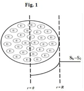
[image:2.596.162.448.405.714.2]

We assume the polymer/enzyme droplet takes a hemispherical shape on an insulting plane, into which the microdisk is inlaid (Fig-1). When enzymes are immobilized on the internal surface of a porous spherical support, the substrate diffuses thorough the pathway among the pores, and reacts with the immobilized enzyme. The mathematical formulation of the microdisk biosensor is described in Phanthong and Somasundrum et al.[9]. It is assumed that the enzyme concentration is uniform and the enzyme reaction follows Michaelis-Menten kinetics, in which case the reaction in the filmis [9]

2 k

1 k

k

1 [E S] P E

E S

cat 1

2

+

+



→

(1)

If the solution is stirred uniformly, so that the substrate S is constantly supplied to the film. At non steady state,the mass balance for S will be given by the equation (2) [9].

t c K

c c c K R c R R R

D _S

M S

S E cat S

2 2

S

  = + −    

 

  



(2)

where

c

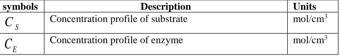
_Sis the concentration profile of substrate, c_Eis the concentration profile of enzyme,

D

_Sis its diffusion coefficient, and K_Mis the Michaelis constant, defined as

K

_M

=

(

k

₋₁

+

k

_cat

)

k

₁

.

Then the initial and boundary conditions at the electrode surface and at the film surface

( )

r₁ are given by

0

c

,

0

t

=

_s

=

(3)

0 R c 0

R S =

 

= (4)

* S S

1 c c

r

R= = (5)

wherec*_S is the bulk concentration of S scaled by the partition coefficient of the film.The boundary condition at R=0 ensures that the substrate distribution is symmetric at the center of the sphere where as the boundary condition at R=r₁ states that the substrate at the surface of the sphere is constant [11].

By defining the following dimensionless parameters * S S

2 1 E cat *

S M 2

1 S 1

* S S

c D

r c K k ; c K ;

r t D ; r

R r ; c c

u= =  =  = =

(6) dimensionless nonlinear equation in a biosensor can be written as follows [1,9]:



 

 = + −   + 

 u

u 1

u k r u r 2 r

u 2 2

(7)

whereu is dimensionless concentration of substrate,kandare reaction constant. This type of equation (Lane Emden equation) also has been used to model several phenomenain mathematical physics and astrophysics [12-15] and the references cited therein. The dimensionless initial and boundary conditions are represented as follows [16]:

0 u ,

0 =

=

 (8)

0 r u , 0

r =

 

= (9)

, 1 u , 1

3. APPROXIMATE ANALYTICAL EXPRESSION FOR THE CONCENTRATION USING HPM

A great number of problems in natural and engineering sciences have been modeled by nonlinear differential equations [17].Homotopy perturbation method is the recent advance methodused to solve manynonlinear equations [18-20]. The basic principle of this method is described in Appendix A. We have obtained the analytical expression of the concentration of substrate by solving the nonlinear equation (1)using new approach of homotopy perturbation method(Appendix B&C).

( )

( )



(

)









 = + − _{− +}       + − + = 1 n 2 2 2 2 1 n m n exp m n ) r n sin( n ) 1 ( r 2 m sinh r r m sinh ) , r (

u  

  

 (11)

wherem=k/(1+



). (12)

The above equation (11) satisfies the boundary conditions (9) and (10) whereas it satisfies the initial condition approximately when m>25. When m=0 or k=0 (there is no reaction) Eqn.(11) becomes  −       − + =  = + − 1 2 2 1 ) exp( ) sin( ) 1 ( 2 1 ) , ( n n n n r n r r r

u  

 

 (13)

This is the well-known solution of Eqn.(7) when k=0. Limiting cases:

Limiting case1: Unsaturated (first order) catalytic kinetics.

We initially consider the major limiting situation where the substrate concentration in the film

) , r (

u  is less than the Michaelis constant k. In this case the productu1. Hence Eqn. (7) reduces to   k r u r 2 r u u 2 2 −   +   =   (14)

Solving the above equation using the initial and boundary conditions (Eqns.(8) to (10)), we can obtain the concentration of substrateas follows (Appendix D):

(

)

( )

e sin(n r)

n 1 r k 2 r 1 6 k 1 ) , r ( u 1 n n 3 n 3

2



2 2

 = − − − − − =        (15) The alternative form of expression of concentration for small values of is

      + + −       + − − =



 =        2 r ) 1 n 2 ( erfc i 2 r ) 1 n 2 ( erfc i r k 4 k ) , r ( u 2 0 n 2 (16) Limiting case 2: Saturated (zero order) catalytic kinetics

Now we consider the next major limiting situation where the substrate concentration in the film

) , r (

u  is greater than the Michaelis constant k. In this case u1 and Eqn. (7) reduces to u k r u r 2 r u u 2 2 −   +   =    (17)

Solving the above equation using HPM for the boundary conditions (8) to (10), we get the following expression for the concentration [21].

( )

( )



(

)









 = + − _{− +}       + − + = 1 2 2 2 2 1 exp ) sin( ) 1 ( 2 sinh sinh ) , ( n n k n k n r n n r k r r k r

u  

  

 (18)

( )

( )

k

r

r k r

u

sinh sinh )

,

(  = (19)

4. NUMERICAL SIMULATION

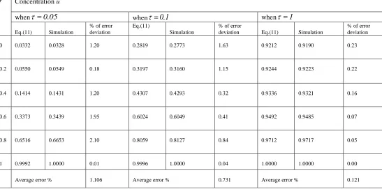
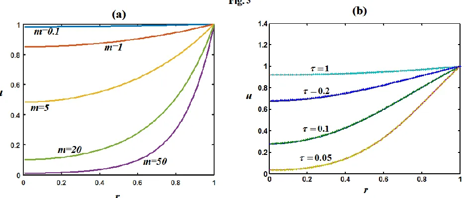
The nonlinear reaction diffusion equation (1) for the corresponding initial and boundary conditions (Eqns.(2)-(4)) are also solved numerically by using Scilab program (Appendix E). The numerical solutions are compared with our analytical results in Table-1 and Fig.3(b) and satisfactory agreement has been noted.

Table 1. Comparison of normalized non steady-state concentration u with simulation results for various values of



and for some other fixed values of parameters

(

k =1 and



=1

)

r _{Concentration u}

when =0.05 when =0.1 when =1

Eq.(11) Simulation

% of error deviation

Eq.(11)

Simulation

% of error

deviation Eq.(11) Simulation

% of error deviation

0 0.0332 0.0328 1.20 0.2819 0.2773 1.63 0.9212 0.9190 0.23

0.2 0.0550 0.0549 0.18 0.3197 0.3160 1.15 0.9244 0.9223 0.22

0.4 0.1414 0.1431 1.20 0.4307 0.4293 0.32 0.9336 0.9321 0.16

0.6 0.3373 0.3439 1.95 0.6024 0.6049 0.41 0.9492 0.9485 0.07

0.8 0.6516 0.6653 2.10 0.8059 0.8127 0.84 0.9712 0.9717 0.05

1 0.9992 1.0000 0.01 0.9996 1.0000 0.04 1.0000 1.0000 0.00

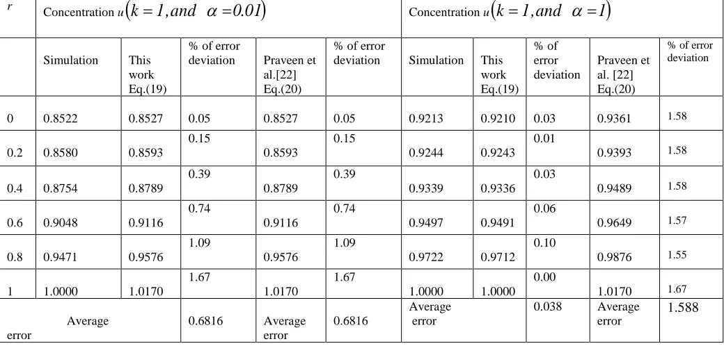
[image:5.596.25.572.340.611.2]

Table 2. Comparison of normalized steady-state concentration u with simulation results for various values ofparameters .

r _{Concentration u}

(

_k=_1,and



=_0.01

)

_{Concentration u}

(

_k=_1,and



=₁

)

Simulation This work Eq.(19)

% of error

deviation Praveen et al.[22] Eq.(20)

% of error

deviation Simulation This work Eq.(19)

% of error deviation

Praveen et al. [22] Eq.(20)

% of error deviation

0 0.8522 0.8527 0.05 0.8527 0.05 0.9213 0.9210 0.03 0.9361 1.58

0.2 0.8580 0.8593

0.15

0.8593

0.15

0.9244 0.9243 0.01

0.9393 1.58

0.4 0.8754 0.8789

0.39

0.8789

0.39

0.9339 0.9336 0.03

0.9489 1.58

0.6 0.9048 0.9116

0.74

0.9116

0.74

0.9497 0.9491 0.06

0.9649 1.57

0.8 0.9471 0.9576

1.09

0.9576

1.09

0.9722 0.9712 0.10

0.9876 1.55

1 1.0000 1.0170

1.67

1.0170

1.67

1.0000 1.0000 0.00

1.0170 1.67

Average error

0.6816 Average error

0.6816

Average error

0.038 Average error

1.588

5. DISCUSSION

Equation (11) represent the concentration profile of substrate as a function of



and r , c , c , K , K ,

D 1

* S E cat M

S . In constant value of initial substrate concentration, enzymatic reaction

rate is a function of

K

_cat

and

c

_E

.

By reducing K_Mor increasing

K

_cat

c

_E, the rate of enzymatic reaction increases, and consequently, the substrate’s concentration reduces in various layers of the spherical support. Recently Praveen et al.[22] obtained the analytical expression of concentration for steady state condition using ADM as follows:

4 2 2 2 2

r 960

k r 288

k 12

k 360

k 7 12

k 1 ) r (

u _

     +    

 

− + + − =

(20)

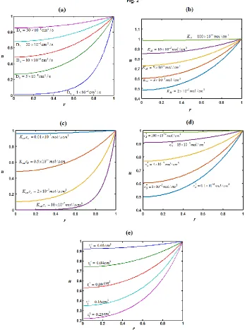
[image:6.596.45.565.114.363.2]

Figure 2 Profiles of the normalized concentration u versus dimensionless distance r calculated using equation (11) for various values of parameters.

3 5

M 3 7

E cat 3

8 *

S 2 2

1 0.01cm , c 3 10 mol/cm , 1, K c 1 10 mol/cm , K 2 10 mol/cm r

) a

( = =  − = =  − =  −

3 5

M 3 9

E cat 2

6 S

2 2

1 0.01cm , D 1 10 cm /s, 1, K c 1 10 mol/cm , K 2 10 mol/cm r

) b

( = =  − = =  − =  −

3 5

M 3 9

E cat 3

6 *

S 2 6

S 1 10 cm /s, c 1 10 mol/cm , 1, K c 1 10 mol/cm , K 2 10 mol/cm D

) c

( =  − =  −  = =  − =  −

3 5

M 3 6

* S 2

7 S

2 2

1 0.001cm , D 10 10 cm /s, 1, c 3 10 mol/cm , K 7 10 mol/cm r

) d

( = =  − = =  − =  −

2 2

1 3 7 E

cat 3

8 *

S 2 6

S 10 10 cm /s, c 3 10 mol/cm , 1, K c 1 10 mol/cm , r 0.01cm

D ) e

[image:7.596.122.469.88.555.2]

Figure 3.(a).Substrate concentration with respect to distance for various values of m when  =1 (b).Substrate concentration with respect to distance for various values of time when

1 and 1

k =



= .

5.1 Effect of the diffusion coefficient on substrate concentration

Effect of the diffusion coefficient

D

_S on substrate concentration is shown in the Figure 2(a).With effective diffusivity increasing, substrate diffuses further and further in the interior layers of support and thus substrate profile gradient decreases when

D

_S increases from

. / 10

50 /

10

1 6cm2 s to 6cm2 s

D_S =  −  −

Diffusion coefficient reduction increases the difference of substrate concentration between the bulk medium and the center of immobilized enzyme support due to increasing of mass transport resistance through the immobilized enzyme. Also the substrate concentration equals to zero in the center of the support when D_S =110−6cm2/s (see Figure 3a).

5.2 Effect of Michaelis-Menten constant K_M on concentration of substrate

The Michaelis-Menten constant is the substrate concentration, which is at half-maximum in the reaction rate. The value of K_M is related to the substrate, enzyme, pH and temperature. The influence of K_Mhave been shown on concentration of substrate in Figure 2(b).A low value of K_M suggests that the enzyme has a high affinity to react with the substrate; so, the substrate's concentration should be decreased with reduction of Michaelis-Menten constantK_M.

5.3 Effect of enzyme reaction rate

(

K

_cat

c

_E

)

on concentration of substrate

[image:8.596.70.537.76.276.2]

the value of

K

_cat

c

_E, concentration of substrate reduces in the porous support and thus the substrate profile gradient increases. Concentration profile in various values of maximum reaction rate is shown in Figure 2(c). In the center of the support, substrate's concentration is zero when

. / 10 8mol s cm3 c

K_{cat E} = −

5.4 Effect of initial substrate concentrationc on concentration of substrate *_S

Based on Fick's law, by increasing the initial concentration of substrate in the bulk medium, concentration profile gradient increases between the center of the support and the bulk medium, and so the substrate diffuses into the support more quickly. As seen in Figures 2(d), initial substrate concentration is effective concentration profile. Substrate concentration approaches to 0 in half radius of the support when c*_s =10−8mol/cm3, and increasing of the initial concentration increases the substrate concentration in the layers of matrices.

5.5 Effect of radius r on concentration of substrate

The influence of radius on concentration of substrate is described in Figure 2(e). From the figure it is inferred that when radius increases the concentration at the center of the sphere is also decreases. From this figures it is also observed that the concentrations substrate are depleted at the center of the microsphere (r=0) as they are consumed by the enzyme reaction.

6. CONCLUSIONS

The non-steady state concentration at a microdisk enzyme based biosensor with Michaelis-Mentenkinitics has been discussed in some detail. Approximate analytical solution to the nonlinear reaction diffusion equation have been presented. In particular a novel and closed -form of approximation has been developed that can be used to integrate the reaction diffusion equation. The theoretical model presented for the non-steady state responds has been used to quantify the steady state substrate response profile. Good agreement was obtained between numerical and theoretical results. The effects of various fundamental kinetic parameters such as Michaelis-Menten constant, diffusion coefficients, enzyme reaction rate and bulk concentration on the concentration of substrate is discussed. By a proper transcription of variables, this method will be extended to derive concentration at microdisk biosensor and rotating disc electrodes with convective and diffusive processes.

ACKNOWLEDGEMENT

Appendix A: Basic Concepts of the HPM

The HPM method has overcome the limitations of traditional perturbation methods. It can take full advantage of the traditional perturbation techniques, so a considerable deal of research has been conducted to apply the homotopy technique to solve various strong non-linear differentialequations. To explain this method, let us consider the following nonlinear differential equations:

0 ) r ( f ) u ( N ) u (

L + − = (A1)

By the homotopy technique, we construct a homotopyv(r,p):[0,1]→Rthat satisfies: 0 )] r ( f ) v ( N [ p ) u ( pL ) u ( L ) v ( L ) p , v (

H = − ₀ + ₀ + − = (A2)

wherep[0,1]is an embedding parameter, and

u

₀is an initial approximation of Eq.(A1)that satisfies the boundary conditions.

When p= 0, Eq.(A2) become linear equation. When p=1,they become nonlinear equation. The process of changing p from zero to unity is that of

L

(

v

)

−

L

(

u

₀

)

=

0

to L(v)+N(v)− f(r)=0. We first use the embedding parameter p as a “small parameter” and assume that the solutions of Eqs.(A2) can be written as a power series in p:

... v p v p v

v= ₀+ ₁+ 2 ₂+ (A3)

Setting p=1 results in the approximate solution of Eq.(A1): ... v v v v lim

u _{0 1 2}

1

p = + + +

=

→ (A4)

This is the basic idea of the HPM.

Appendix B: Approximate Analytical Solution Eqn.(12) using HPM Method We construct the new homotopy for the Eqn.(12) as follows [15]:

0 ku u r u r 2 r u ) u 1 ( p u ) ) 1 x ( u 1 ( u k r u r 2 r u ) p 1 ( 2 2 2 2 =         −         −   +   + +         − = + −   +   −     (B1)

wherep[0,1]is an embedding parameter. Now assume that the solution of the Eqn. (1) is



+ +

+ +

= 3 ₄

2 2 1

0 pu p u p u

u

u (B2)

Substituting the above eqn. (B2) in eqn. (B1) and equating the like coefficient of pon both side we obtain: 0 u u 1 k r u R 2 r u : p 0 0 0 2 0 2 0 =   −       + −   +     (B3)

In Laplace plane this equation becomes: 0 u ) s m ( dr u d r 2 dr u d 0 0 2 0 2 = + − + (B4) where  + = 1 k

m and s is a Laplace variable. The boundary conditions become: 0 dr u d , 0

r= 0 =

(B5) s 1 u , 1

r = ₀ = (B6)

R u Q dr

u d P dr

u d

0 0 2

0 2

= +

+ (B7)

Where P, Q, Rare function of R. Using reduction of order, from eqn. (B1), we have 0

R and ); s m ( Q ; r 2

P= =− + = (B8)

Let

u

₀

=

vw

(B9)

be the general solution of eqn. (B7). If v is so chosen that 0

Pv dr dv

2 + = (B10)

Substituting the value of P in the above eqn. (B10), we obtain: r

1 v= (B11)

Then eqn. (B7) reduces to:

1 1 "

R

w

Q

w

+

=

(B12)

where

v R R ; 4 P dr dP 2 1 Q

Q ₁

2

1 = − − = (B13)

Using eqn. (B8) andeqn. B(7) reduces to:

0 w ) s m ( "

w − + = (B14)

Integrating eqn. (B9) twice, we obtain ) r s m exp( C ) r s m exp( C

w= ₁ + + ₂ − + (B15)

Substituting eqn. (B7) and eqn. B(11) in eqn.(B5), we have:

( )

(

C exp( m sr) C exp( m sr)

)

r

1 s , r

u₀ = ₁ + + ₂ − + (B16)

Using the boundary conditions eqs. (B6) and (B7), we can obtain the value of the constants:

) s m sinh( s 2

1 C

and ) s m sinh( s 2

1

C_{1 2}

+ −

= +

= (B17)

Substituting eqn.(B17) in eqn. (B16), we obtain 

   

  

+ + =

) s m sinh( s

) r s m sinh( r

1 ) s , r (

u₀ (B18)

Appendix C: Inverse Laplace Transform of Eqn. (B18) Using Complex Inversion Formula.

In this Appendix we indicate how equation (B18) may be inverted using the complex inversion formula. If y(s) represents the Laplace transform of a functiony(), then according to the complex inversion formula we can state that:





=

= _+



− c

i c

i c

ds ) s ( y ] s exp[ i 2

1

ds ) s ( y ] s exp[ i

2

1 )

(

y 

 



 (C1)

considering the contour integral presented on the right-hand side of equation (C1), which is then evaluated using the so-called Bromwich contour. The contour integral is then evaluated using the residue theorem which states for any analytic function F(z)



=



= c n z z 0 )] z ( F [ s Re i 2 dz ) z (

F  (C2)

where the residues are computed at the poles of the function F(z). Hence from eqn(C2),we note that:



= = n s s n )] s ( y ] s [exp[ s Re ) (

y  (C3)

From the theory of complex variables we can show that the residue of a function F(z) at a simple pole at

z

=

a

is given by the following equation:

)} ( ) {( ] ) ( [

Res F z

_lim

z a F z

a z a

z = −

→

= (C4)

Hence in order to invert equation (B18) we need to evaluate:

(

)

(

)

      + + s m sinh s r s m sinh s Re

The poles are obtained from

s

sinh

m

+

s

= 0. Hence there is a simple pole at

s

= 0 and there are infinitely many poles given by the solution of the equation

sinh

k

+

s

= 0 and sos_n=−(n22+m) where n = 0,1,2,…….

Hence we note that:

(

)

(

)

s 0 ssinh

(

(

m

)

s

)

s s_n

r s m sinh s Re s m sinh s r s m sinh s Re ) , r ( u = =       + + +       + + =  (C5)

The first residue in equation (C5) is given by the following equation:

(

)



ssinh m s



s 0

s

Re + = =

(

(

)

)



     + +

→ _{ssinh m s}

r s m sinh ) s exp( lim 0 s  = m sinh r m sinh (C6) The second residue in equation (C5) is given by:

(

)



ssinh m s



s s_n s

Re + = =

(

(

)

)



     + +

→ _{ssinh m s}

r s m sinh ) s exp( lim n s s  =

(

)

(

)

_          + + → s m sinh ds d s r s m sinh ) s exp( lim n s s  ... 2 , 1 n , ) in cosh( ) m n ( ) r in sinh( ) in ]( ) m n ( exp[ 2 2 2 2 2 = + − + − =       (C7) Using cosh(i



)=cos(



)and sinh(i



)=isin(



)

) 8 C ( ] ) m n ( exp[ m n ) r n sin( n ) 1 ( 2 ) s m sinh( ) r s m sinh( e Lt 1 n 2 2 2 2 1 n s s

s n



 = + − → _ − +     + − = + + _{ }    

= ) , r ( u



r 2 ) m sinh( r ) r m

sinh( ₊  _

        + −  = + − + −

0 2 2

) ( 1 ) ( ) sin( ) 1

( 2 2

n m n n m n e r n n     (C9)

Appendix D: Analytical Solution of Eqn. (16) Eqn .(13) can be written as

 k r u r 2 r u t u 2 2 −   +   =   (D1) The initial and boundary conditions are

0 r u ; 0 r 1 u ; 1 r 0 u ; 0 =   = = = = =  (D2) when r v

u= , the eqn. (D1) becomes

      −   =    kr r v t v 2 2 (D3)

Now initial and boundary condition becomes

0 v ; 0 r 1 v ; 1 r 0 v ; 0 = = = = = =  (D4) Let  6 r k w v 3 + =

Now equation(D3) becomes 2 2 r w t w   =   (D5)

Initial and boundary condition becomes

0 w ; 0 r 6 k 1 w ; 1 r 6 r k w ; 0 3 = = − = = − = =    (D6)

The solution of eqn.(D5) becomes



 = − − −       − = 1 n 2 2 3 n

3 sinn rexp( n )

n ) 1 ( k 12 r k 1 ) , r (

w   

   (D7) ) n exp( r r n sin n ) 1 ( r k 2 ) r 1 ( 6 k ) , r (

v 2 2

1 n

3 n 3

2   

    =− − −



 − − = (D8) ) n exp( r r n sin n ) 1 ( k 2 6 kr 6 k 1 ) , r (

u 2 2

Appendix E: Scilab Program to Find the Numerical Solution of Eqn. (1) function pdex2

m = 2;

x = linspace(0,1); t=linspace(0,100);

sol = pdepe(m,@pdex2pde,@pdex2ic,@pdex2bc,x,t); u1 = sol(:,:,1);

[image:14.596.131.463.717.772.2]

%--- figure

plot(x,u1(end,:)) title('u1(x,t)') xlabel('Distance x') ylabel('u1(x,1)')

%--- function [c,f,s] = pdex2pde(x,t,u,DuDx)

c = [1; 1; 1];

f = [1; 1; 1] .* DuDx; a=10;

k=2;

F= (- g*u(1)*u(2))*((a*u(2)+u(1)*u(2)+u(1)*b)^(-1)); s=[F];

% --- function u0 = pdex2ic(x)

u0 = [1; 0; 0];

% --- function [pl,ql,pr,qr]=pdex4bc(xl,ul,xr,ur,t) pl = [ul(1)-0; ul(2)-0; ul(3)-0];

ql = [1; 1; 1];

pr = [ur(1)-1; ur(2)-1; ur(3)-0]; qr = [0; 0; 0];

Nomenclature

symbols Description Units

S

C

Concentration profile of substrate mol/cm3

E

* S

C

Concentration of profile in the external solution mol/cm3

S

D

Diffusion coefficient _cm2 _/s

cat

K

Kinetic enzyme reaction rate 1 sec−

M

K

Michaelis-Menten constant mol/cm3

F

Faraday constant Cmol-1

 Dimensionless time None

A Surface area of the electrode 2 cm

1

r

Radius of the electrode 2

cm

t Time S



&

k Dimensionless reaction diffusion parameters None

r Dimensionless radius None

u Dimensionless of Concentration profile None

References

1. L.Rajendran, Chemical Sensors: Simulation and Modeling Volume 5: Electrochemical sensors, Edited by GhenadiiKorotcenkov, Momentum Press,(2013), Newyork, ISBN:9781606505960 2. I.Ismail, G.Oluleye, I.J Oluwafemi, O. Iomofuma, A. Solufemi, International Journal of

Biosensors & Bioelectronics, 3(2)(2017) 00062.

3. R. Baronas, F. Ivanauskas, I. Kaunietis, V. Laurinavicius, Sensors, 6(7)(2006) 727. 4. A. Eswari, L.Rajendran, J.Electroanal. Chem., 651(2011)173.

5. K.Saravana Kumar, L.Rajendran, International Journal of Mathematical Archive, 2(11) (2011) 2347.

6. S.Dong, X. Xi, M.Tion, Electroanal.Chem., 309 (1991) 103.

7. M.E.G. Lyons, T. Bannon, S. Rebouillat, The Analyst, 123 (1998) 1961. 8. J.Galceran, S.L.Taylor, P.N Bartlett, J. Electroanal. Chem., 506(2001)65. 9. C.Phanthong, M.Somasundrum,J. Electroanal. Chem., 558(2003) 1 10.L. Rajendran, S.Anitha, Electrochim.Acta, 102(2013) 474.

11.S. Rebouillat, M.E.G. Lyons, A. Flynn, The Analyst, 124 (1999) 1635. 12.A.M. Wazwaz, Chem. Phys. Lett., 679 (2017)132.

13.A.M. Wazwaz and R. Rach, Kybernetes., 40(9/10) (2011)1305. 14.R.Singh, N. Das, J. Kumar, EurPhys J Plus., 132 (6) (2017)251. 15.R. Duggan, A. Goodman, Bull Math Biol., 45(5) (1983) 661.

16.M E.G. Lyons, T. Bannon, G. Hinds, S. Rebouillat, The Analyst, 123 (1998) 1947. 17.J. H.He, W.X. Hong, Chaos, Solitons&Fractols, 29 (2006) 108.

18.J.H.He, X.H. Wu, Computers & Mathematics With Applications, 54 (2007)881.

19.J. Visuvasam, A. Molina, E. Laborda, L. Rajendran, Int. J. Electrochem. Sci., 13 (2018) 9999. 20.R.A. Joy, A. Meena, S. Loghambal, L. Rajendran, Natural Science, 3(7) (2011) 556.

21.M. Rasi, L. Rajendran, M.V Sangaranarayanan, J Electrochem Soc., 162(9)(2015)H671. 22.T. Praveen, Pedro Valencia, L. Rajendran, Biochem. Eng. J., 91(2014)129.