Rochester Institute of Technology
RIT Scholar Works
Theses Thesis/Dissertation Collections
2008
Solving an MRI spin relaxometry problem using
Parallel Java
Hardik Parikh
Follow this and additional works at:http://scholarworks.rit.edu/theses
This Master's Project is brought to you for free and open access by the Thesis/Dissertation Collections at RIT Scholar Works. It has been accepted for inclusion in Theses by an authorized administrator of RIT Scholar Works. For more information, please contactritscholarworks@rit.edu.
Recommended Citation
Project Report
Topic:
Solving MRI Spin Relaxometry Problem (using PJ)
Student:
Hardik J. Parikh
Committee:
Chair: Prof. Alan Kaminsky
Reader: Prof. Paul Tymann
Abstract:
Magnetic resonance imaging (MRI) is an imaging technique used primarily in the medical profession to produce high quality images of the inside of the human body, without using x-rays. The process of obtaining the spin density spectrum from the time samples of the spin signal for each pixel of a magnetic resonance image is known as MRI Spin Relaxometry [5]. The spin density spectrum is obtained by performing linear regularization on samples of magnetic resonance images obtained at different times. The spin density spectrum obtained from the body, is used by radiologists to diagnose disease, in its early stages.
1
Overview
1.1
Magnetic Resonance Imaging (MRI)
Magnetic resonance imaging (MRI) is a technique, used by radiologists, to produce high quality images of the inside of the body. MRI uses electromagnetic waves and radio frequencies (a.k.a. RF’s) to produce images of the inside of the human body that can be used to diagnose a disease in the early stages. Tissues in the body have spin-lattice relaxation rate (R1) and spin-spin relaxation rate (R2). The distribution of R1 and R2 generates a signal from which an image is generated. R1 and R2 are said to possess diagnostic utility because the rates differ in a healthy tissue as compared to a diseased tissue. Hence the disease can be diagnosed from the image of the organ.
An MRI scanner is a device that produces a two-dimensional image of the part of the human body that is being scanned. The MRI scanner sends magnetic pulses (RF signals) through the body, and captures the images sequence to generate one slice of an image. By taking several images from different angles, a three-dimensional image is constructed. Thus, each slice’s data comprises M images, which are taken at time values t and consist of an image comprised of R * C pixels [5].
1.2
MRI Spin Relaxometry Problem
The problem here is to find the spin density spectrum from the noisy MRI signal. Thus, this is the inverse problem i.e. figuring out the input that generated the known output. The dependency between the spin relaxation rate (x) and spin density (ρ) is non-linear. According to the inversion recovery sequence, the dependency is shown by equation
S (t) = ρ (1 – 2e-xt) (1)
ρ = spin’s density
x = spin’s relaxation rate (sec-1)
t = time at which image was taken (sec)
Figure 1
Thus, if there are two tissues, then the diagram becomes as shown below when ρ1 = 750, x1 = 1.5 for tissue 1, ρ2 = 250 and x2 = 0.5 for tissue 2. The resulting pixel’s signal value S, at a given time t, is the summation of signals from all different kind of tissues, as depicted in the diagram shown below, for the tissues with above stated values. Thus, the signal value S, at time t is
S (t) = ∑ρ (1 – 2e-xt) (2)
where ρ is the spin density and x is the relaxation rate, across all the tissues.
Figure 2
[image:5.612.122.494.419.625.2]Figure 3
Real MRI scans would not have this many discrete values of ρ at various values of x. Instead, the values of ρ will be clustered around the possible values of x. Thus, in reality, what is depicted above, would look as shown below
Figure 4
The ρ is a continuous function of x. Thus, equation (2) transforms to the following equation
S (t) = ∫ρ(x) (1 – 2e-xt) dx (3)
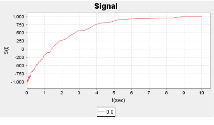
[image:6.612.122.494.365.576.2]Also, the signal diagrams are not ideal as depicted in Figure 1 and Figure 2. There are some measurement errors induced due to MRI instruments. Thus, the original signal obtained looks somewhat as shown below
Figure 5
Thus, the MRI Spin Relaxometry problem is obtaining spin density spectrum ρ(x) values from value of signal S(t) at time t. It is an inverse problem, because from output, we have to track back the input value that generated the output. This has to be done for each pixel of an MRI image because each pixel contains an unequal number of tissues and thus different spin spectra.
2
Previous work done:
Some work has been done in the area of solving MRI Spin Relaxometry problem.
1. Running serial algorithms simultaneously
Dr. Hornak, along with Prof. Schaller, tried to solve the problem by running parallel (more than one) versions of the serial algorithm that was used to solve the MRI Spin Relaxometry problem. Thus, multiple serial algorithms were run at the same time. More information can be obtained at [4].
2. Running a parallel algorithm [5]
3
Design Specifications
There are basically two methods for solving the problem and finding ρ(x) values.
1. Selecting the values of spin relaxation rate (x) in some acceptable range and then using a particular method like constrained linear regularization and finding a non-negative least squares solution. Here the values of the rate (x) are known and we try to find the spin density (ρ(x)). This particular method was used by Prof. Kaminsky to solve the problem.
[image:8.612.42.570.267.613.2]2. Figuring out the values of ρ(x) and x, at the same time. The relationship between both is linear, as seen in equation (3). Thus, we need to perform the non-linear least squares approach and obtain the non-negative least squares solution.
Figure 6: Architectural Overview Diagram
We have used the same MRI dataset that was used in [5]. The output file generated by our Linear Regularization approach is exactly the same as the one generated in [5]. The sequential programs are also implemented along with their parallel versions for doing performance comparison and calculating speed-ups. With the help of this project, we are trying to do two specific comparisons:
MRI Input Data Set Linear Regularization Analysis Program (parallel, C/MPI) Linear Regularization Analysis Program (parallel, Java/PJ) Linear Regularization Visualization Program (Non-parallel, Java) Non-Linear Least Squares Analysis Program (parallel, C/MPI) Non-Linear Least Squares Analysis Program (parallel, Java/PJ) Linear Regularization Output Dataset Non-Linear Least Squares Visualization Program (Non-parallel, Java)
• Linear regularization vs. non-linear least squares algorithm – We are passing the same MRI input dataset to two different algorithms and comparing the efficiency and speed of two algorithms. We also compare the output results.
• Java vs. C – We are also comparing the running times of Java and C versions.
The output files we generate for linear regularization and Non-linear least squares algorithms are also different. We provide this output file to the visualization programs corresponding to those algorithms.
4
Constrained Linear Regularization Approach
For linear regularization, the output function g(y) is defined in terms of an input function f(x) and a response kernel r(x, y) as:
g(y) =
∫
f(x)r(x,y)dx (4)The continuous integration at all the points is approximated by the summation of the values at discrete points.
∑
= = N j i j ji f x r x y
y g 1 ), , ( ) ( )
( for i = 1, 2 ….M (5)
Now, if we have the M values ofyi, N values ofxj, the measurement samples of the function g(yi)(which possibly include measurement errors), and the response kernel valuesr(xj,yi), then the inverse problem here is to find the function values f(xj)which
generated the output samples.
From equation (3), it can be seen that the dependency between the spin relaxation rate (x) and spin density (ρ) is non-linear. Using linear regularization approach [10], the spin density values (ρ) can be found if all the other parameters are known. Thus, if we have the value of the spin signal S(t) and the spin-relaxation rates (x), then the spin density (ρ) can be found.
This approach was explored by Prof. Kaminsky and Luke McOmber [5] to design the program that takes the spin relaxation rate values (x) in an acceptable range and finds out the corresponding spin-density values, such that the reconstructed signal S)(t)(from the obtained ρ and value of x) matches as closely as possible to the original signal value S(t).
4.1 Input Files
This section describes the input files for the MRI spin relaxometry problem. There are times file, a number of image files, and a mask file.
4.1.1
Times File
Times file is a text file and it provides the image dimensions (in terms of number of pixels) and the timings at which the images were taken. Each line of times file is separated white space.
The first line of the times file has two fields: the total number of rows R (integer) of the image and the total number of columns C (integer) of the image. The rest of the times file consists of M lines. Each line contains two fields. The first field gives time ti (sec, real
number) at which the image i was taken, 1<= i<= M. The second field gives the name of the image file for image i.
4.1.2
Image File
Image file is a binary file containing the image pixel values for a particular image i taken at time ti. The file contains total R x C pixel values Src(ti), where r is the row number
(0<= r <= R-1) and c is the column number (0 <= c <= C-1). The pixels are stored in the row major order i.e. the values of first row from left to right, the values of second row from left to right and so on.
Each pixel value is stored in binary as a two-byte integer in the range -32768 <= Src(ti) <=
32767. The first two pixel values (S00 and S01) do not contain actual data but they are set
to S00 = 0 and S01 = 1, which helps in deciding the endianness with which the pixels are
stored. Thus, if the first four bytes of image file are 0, 0, 0 and 1, then the pixels are stored in big-endian format i.e. the most significant byte first. If the first four bytes of image file are 0, 0, 1 and 0, then the pixels are stored in little-endian format i.e. the least significant byte first.
4.1.3 Mask file
The mask file is a binary file containing R x C pixel mask values Mrc. Mrc is 1 if pixel
(r; c) has data to be analyzed. Mrc is 0 if pixel (r; c) is not to be analyzed. Masking out
certain pixel reduces the time needed to do the analysis.
Each mask value is stored in binary as a two-byte integer. The first pixel (M00) does not
contain actual mask data, but instead is set to the value M00 = 1. This is used to determine
the mask value’s byte order. If the first two bytes of the mask file are 0, 1, then the mask values are stored in big-endian order. If the first two bytes of the mask file are 1, 0, then the mask values are stored in little-endian order.
4.2
Sequential Analysis Programs (C & Java)
The sequential analysis program for Java remains the same as in [5]. The program SRSolveSeq is not changed at all and is used to do performance comparison with sequential analysis program for C. The sequential C program (SRSolveSeqC) is merely translated from the sequential Java program into C language.
The sequential programs (in C as well as Java) are created to do performance comparison between C and Java, as well as provide a benchmark for the performance comparison for their counterpart parallel programs.
The parameters for the programs remain common and are actually the same parameters, as provided for the SRSolve program [5]. The parameters are:-
• xL,xU,N- The programs calculate the spin densities for N values of spin relaxation rate xspaced between xLand xU inclusive.
•
λ
L,λ
U,L- The programs calculate the solution for L values of the tradeoffparameter λ spaced logarithmically between
λ
Landλ
Uinclusive.• times – The name of the file which contains timings of all the images data.
• mask – The name of the mask file for image data.
• output – The name of the output file in which the analysis results will be stored
• description – The description to be included in the output file.
The data fed into the programs was also the same used in [5], with xL= 0.02, xU = 2.0, N
= 100,
λ
L= 1e-3,λ
U= 1e2, and L = 16.Now, because the programs are sequential, there is only one process working on the programs at a time. The process reads the times file to determine the names of the input
image data files. The process also reads the mask file to determine the total number of unmasked pixels. Now the process reads the spin signal values from the input image files and for each pixel, the solution
ρ
ˆ(x)is computed.ρ
ˆ(x) is calculated for all the λ betweenL
λ
andλ
U, using the constrained linear regularization algorithm (described in [5]). The corresponding F statistic and significance Q statistics for thatρ
ˆ(x) are also computed (described in [5]). The results are written to the file named output (given at the command line).The format of the output file is described in Section 4.4.
4.3
Parallel Analysis Programs (C & Java)
Java Program
We wrote PJLinearRegularization program, which is a parallel program, in Java (using PJ). The Java program is a mere translation of the SRSolve program of [5]. Instead of the mpiJava that Prof. Kaminsky and Luke McOmber used, we have used the PJ library to induce parallelism. This program reads the input files, calculates the solution using the Linear Regularization algorithm and writes the output to a file.
C program
For comparison with the Java program, we also wrote a SRSolveC program, which is a parallel program in C (using MPI). The functionality of this program is exactly similar (for exact comparison) to the corresponding java program. The algorithm that this program uses is also the same i.e. linear regularization algorithm.
The parallel programs run on a cluster parallel computer with K processes operating on the programs simultaneously. Each process runs on a different processor and is assigned a rank between 0 and K - 1.
Each process reads the times file to determine the names of the input image data files. Each process also reads the mask file to determine the unmasked pixels. The total number of unmasked pixels is divided equally among the processes. If the number of pixels cannot be divided equally among the processes, then they are divided such that the difference between the total number of pixels analyzed by any two processes is 1. Thus, maximum possible proper load balancing is ensured. Now, each process reads the spin signal values for its subset, from the input image files. For each pixel, the assigned process computes the solution
ρ
ˆ(x)for all the λ betweenλ
Landλ
U, using the constrained linear regularization algorithm (mentioned in Section 4 and 5). The process also computes the F statistic and significance Q statistics for thatρ
ˆ(x). Each process writes its results in the file with name of type “output_rank” where output is specified at the command line and rank is the rank of the corresponding process. Thus, if there are 4 processes operating on the programs, then the file names would be “output_0”, “output_1”, “output_2” and “output_3” (because the process rank starts with 0).There is no communication between the processes. Hence near-ideal speedups are expected as the number of processes increases.
4.4 Output File Format
The output file generated by the programs is also a binary file and the data is stored as a multi-byte quantity. An int and a float value occupy 4 bytes. The contents of the output file are as follows:
• Description (string; from the command line of programs)
• Number of Rows in the image, R (int)
• Number of time values, M (int)
• Time values, ti(M floats)
• Number of spin relaxation rates, N (int)
• Spin relaxation rate values, xj(N floats) • Number of tradeoff parameter values, L (int)
• Tradeoff parameter values,
λ
k(L floats)• Number of pixels in this file, P (int)
• Pixel indexes in this file (P ints)
• For each pixel:
- Spin signal values, Si (M floats)
- For each tradeoff parameter value - F statistic (float)
- Significance of F statistic, Q (float) - Spin density values, ρj(N floats)
For the generation of the file, the same MRI test data is used as in [5]. The program generates an output file of 16.8 megabytes.
4.5 Linear Regularization Visualization Program
To do further analysis, we calculated the spin densities (ρj) and obtained the corresponding spin relaxation rates (xj) at the lowest value of λ provided at the command line. Thus, we chose λ =
λ
L= 1.0 x 10⁻³
. Now, as explained in [5], due to such a low λ value, the solution vector (
ρ
ˆ(x)) obtained was not smooth because of the random fluctuation errors. The PJLinearRegularization program generates the solution vector for all the unmasked pixels.The solution vector contains N float values of ρ(x) (at each of the spin relaxation ratesx). From the solution vector of each pixel, we extracted the ρ(x)(spin-density) and its corresponding x(spin relaxation rate) values where ρ(x) > 0.
Now, a histogram [8] is generated of all the spin-relaxation rate values obtained to see the total count of each spin-relaxation rate. The main purpose of generating the histogram is to find the area of major concentration of spin-relaxation rates. The histogram chart is generated using the JFreeChart utility [9].
5
Non-linear Least Squares Approach
Referring back to equation (2), the overall spin signal is the summation of the spin signals for all the tissues. Thus, the final spin signal measurement with K tissues and taken at time t (secs) can be given as:
∑
= − − = K j t x j j e x t S 1 ) 2 1 ( ) ; ;(
ρ
ρ
(6)Now, the
ρ
=ρ
1,ρ
2,....ρ
K can be considered as a vector of tissues spin densities andK
x x x
x= 1, 2,... as vector of spin relaxation rates.
Unlike the approach discussed in Section 4, we can calculate the spin densities ρ and the spin relaxation rates x at the same time using the non-linear least squares algorithm. An implementation of Levenberg-Marquardt method [10] is used.
In the implementation of the algorithm, parameter vector a is defined as:
K K x x x
a=
ρ
1,ρ
2,....ρ
, 1, 2,... , where (7)j j K j
j a x
a =ρ , + = for all j = 1, 2, … K (8)
Thus, equation (6) can now be represented in terms of parameter vector a as:
∑
= − + − = K j t x j j K e a t S 1 ) 2 1 ( ) ;(
ρ
(9)More information about the algorithm can be found at [10], chapter 15.5.
5.1 Input files
The input files used are the same as ones discussed in Section 4.1.
5.2 Sequential Analysis Programs (C & Java)
The sequential analysis programs try to solve the MRI Spin Relaxometry problem using the non-linear least squares approach. The sequential program implemented in Java (SRSolveNLLSSeq) is exactly the same to the sequential program implemented in C (SRSolveNLLSSeqC). The sequential programs (in C as well as Java) are created to do performance comparison between C and Java; as well as provide a benchmark for the performance comparison for their counterpart parallel programs.
• times – The name of the file which contains timings of all the images data.
• mask – The name of the mask file for image data.
• seed – The random seed (long) used to generate the random double values
• output – The name of the output file in which the analysis results will be stored
• description – The description to be included in the output file.
• xL- The lower bound for the spin-relaxation rate
• xU- The upper bound for the spin-relaxation rate
The program runs sequentially, so there is only one processor working on the problem. As per the implementation of the non-linear least squares algorithm, the parameter vector
a is filled with the double values (between 0.0 and 1.0) generated through the random
number generator for C and Java. The seed is used to initialize this random number generator.
The processor reads the image file and times file. For all the unmasked pixels, a model function is generated, which is the one represented by equation (9). The parameter vector
a is filled the random double values (generated from the random number generator) and
the best-fit parameters i.e. spin density ρ and spin relaxation rate x are found.
To filter out certain unacceptable values ofx, the lower bound xL and the upper bound
U
x are provided as parameters. Thus, it is certain that the x values are within acceptable range. The output of the analysis program, along with its description (provided at the command-line), is written in a file named output (given at the command line).
5.3 Parallel Analysis Programs (C & Java)
As with the Linear Regularization approach, we have also created parallel analysis programs, in C and Java both, for the performance comparison between sequential and parallel programs. Again, the main aim here is the comparison between two difference approach to solve the MRI spin relaxometry problem and also to compare the PJ library with MPI library.
Java Program
We have written the SRSolveNLLSPJ program in Java, using Prof. Kaminsky’s PJ library. The program reads the input files, processes the unmasked pixels using the non-linear least squares algorithm and writes the output to the files.
C Program
These parallel programs run on a cluster parallel computer with K processes operating on the programs simultaneously. Each process runs on a different processor and is assigned a rank between 0 and K - 1.
Each process reads the times file to determine the names of the input image data files and to get the total number of rows and columns in the image. Each process also reads the
mask file to determine the unmasked pixels, so that unnecessary processing of masked pixels is avoided. The total number of unmasked pixels is divided among the total number of processes (given through command-line) operating. Now, each process has a count of its slice of unmasked pixels. The process reads the signal values for only the slice of the unmasked pixels. Then, each pixel’s signal values are passed through the non-linear least squares algorithm and the best-fit parameters are found. For initializing the a
parameter vector, the random values are also independently generated by the processes, using the seed provided from the command-line which initializes the random number generator. Also, from the best-fit parameters obtained, only those values of spin-relaxation rates are kept which fall in the range of bounds provided at the command-line. Each process writes its results in the file with name of type “output rank” where output is specified at the command line and rank is the rank of the corresponding process.
Thus, parallel programs for constrained linear regularization and non-linear least squares are exactly similar until reading of signal values from the files for unmasked pixels. The main algorithm causes the difference between the two approaches.
5.4 Output File Format
The output file generated is a binary file and all the data is written in multi-byte quantities. The values written to the binary file, in sequence, are:
• Description (string; from the command line of programs)
• Number of Rows in the image, R (int)
• Number of Columns in the image, C (int)
• Number of time values, M (int)
• Time values, ti(M floats)
• Number of Pixel indexes in this file (P ints)
• For each pixel:-
- Index of the pixel (int)
- Total number of best-fit parameters value i.e. K (int) - Spin densities
ρ
1,ρ
2,....ρ
K(K floats)- Spin relaxation rates x1,x2,...xK(K floats)
Again, for ideal performance comparison, same MRI test data is used as Section 4 and [5]. The file generated is 705 kilobytes.
5.5 Non-linear Least Squares Visualization Programs
obtained
ρ
1,ρ
2,....ρ
Kare written to the output file, along with the corresponding spinrelaxation ratesx1,x2,...xK. From this output file, we extracted all the spin relaxation rates for all the pixels. Thus, we now have a list of spin relaxation rates
N N x
x x x
x1, 2, 3... −1,, and the length of the list is N.
For creating the distribution plot, the list of spin relaxation rates x1,x2,x3...xN−1,,xN is
sorted. Thusx1has minimum value andxNhas the maximum value. The y-axis of the plot ranges from 0 to 1. Thus the incremental factor for plotting each point is 1/N. Each new spin relaxation rate is plotted as a new (x, y) point whose y-axis value is incremented by 1/N to the y-axis value of the previous (x, y) point. Thus, 1st point is (x1, 1/N), 2nd point is (x2, 2/N), 3rd point is (x3, 3/N) and so on. The last point obtained is (xN, N/N) i.e. (xN, 1).
Thus, by creating a distribution plot, we get an idea of where the region is with major concentration of the spin relaxation rates. Now, wherever there is major concentration of spin relaxation rates, the values are fairly close. Hence the x-axis distance between two points in the plot is considerably less but the y-axis distance remains the same, and the slope in that clustered region is very steep. Thus the steepness of the slope of the distribution plot is directly proportional to the concentration of spin relaxation rates in that region. A higher concentration of spin relaxation rates in a region implies steep slope in the distribution plot for that region.
Density plot basically highlights the areas where spin relaxation rates have more concentration of values. It can also be helpful to figure out the relative difference in concentration of x in various regions. For density plot, we take into consideration a
sliding window parameter such as ω. The x-axis for the plot comprises of all the x values. For a particular point (xi, yi), the x-axis value is the x value, and the y-axis value is the
total number of x values that fall within the range of (xi – ω) and (xi + ω). The density plot
comprises of curve with multiple peaks. The peak with the highest height depicts the region with the highest concentration of x values. Thus, if (xi, yi) is the highest point of
the highest peak in the curve, then the maximum concentration of x values is in the range (xi – ω) and (xi + ω).
6
Results of Analysis
We calculated the timing measurements for each approach (Section 3) and also did the different visualization programs for each approach.
6.1
Linear Regularization Approach Results
For the linear regularization approach, we took the timing measurements and also did a histogram plot for further analysis.
6.1.1
Timing Measurements
For the linear regularization algorithm, a total of four programs were created: the sequential Java program (SRSolveSeq.java), Parallel Java program (PJLinearRegularization.java), sequential C program (SRSolveCSeq.c) and parallel C program (SRSolveC.c). The speed-up measurements of the parallel programs were done on the basis of their sequential counterparts.
The timing measurements were done by running the programs on a 32-processor cluster computer, using the data used in [5]. This is the same cluster computer that was used in [4] and [5]. Each processor in the cluster is a Sun Microsystems 440 MHz UltraSPARC-IIi CPU with 256 MB of main memory. The running time measurements were done when the parallel programs were run on 1, 2, 4, 8, 16 and 32 processors. The sequential programs were also run to create a benchmark for speed and efficiency. Each of the above programs were run five times and the table below shows the average time taken (in seconds) by the programs for creating the output files.
Number of processors (K) Java code time (seconds) C code time (seconds) Speedup (Java) Efficiency (Java) Speedup (C) Efficiency (C)
Sequential 6684 4019
[image:18.612.83.536.453.601.2]1 6853 4098 0.9574 0.9574 0.9807 0.9807 2 3461 2087 1.9314 0.9657 1.9256 0.9628 4 1654 1070 4.0414 1.0103 3.7560 0.9390 8 936 542 7.1416 0.8927 7.4151 0.9269 16 469 281 14.252 0.8908 14.3024 0.8939 32 234 140 28.5662 0.8927 28.7069 0.8971
[image:18.612.87.533.454.600.2]Table 1 – Linear Regularization Analysis Program running times
Figure 7: Linear Regularization Java code speedup
Figure 8: Linear Regularization Java code efficiency
[image:19.612.194.416.508.687.2]Figure 10: Linear Regularization C code efficiency
The above diagrams show the speed-up and efficiency achieved. Also, the C code takes less time as compared to Java code because the Java virtual machine converts the code into byte-code and then interprets into machine language, whereas the C code is compiled directly into machine language.
[image:20.612.107.506.397.702.2]6.1.2
Visualization Plots
Figure-11 below shows the histogram generated.
The x-axis represents the bins of the spin-relaxation rates and the y-axis represents the total count of spin-relaxation rates falling in different bins.
The total number of bins for this histogram is N (which is same as the total number of spin relaxation rates provided when running Linear regularization programs). The first bin ranges from 0.0 to 0.02, the second bin ranges from 0.021 to 0.04, the third bin ranges from 0.041 to 0.06 and so on.
[image:21.612.92.504.233.556.2]As we can see from the above diagram, more concentration of the spin-relaxation rates is between 0.5 and 0.7. Also, the bin from 1.981 to 2.0 contains the maximum number of values, but those values are insignificant as they are due to the random measurement errors in the output vector solution [5]. Figure 12 shows a closer look at the diagram.
Figure 12 – Linear Regularization Histogram (between x= 0.5 and x= 0.7)
From Figure 12, we can see that the maximum count of xis contained in the bin between
6.2
Non-linear Least Squares Approach Results
6.2.1
Timing Measurements
For non-linear least squares algorithm, total of four programs were created: the sequential Java program (SRSolveNLLSSeq.java), Parallel Java program (SRSolveNLLSPJ.java), sequential C program (SRSolveNLLSSeqC.c) and parallel C program (SRSolveNLLSC.c). The speed-up measurements of the parallel programs were done on the basis of their sequential counterparts.
The timing measurements were also done on the same cluster machine that is described in Section 6.1.1. The measurement was done on 1, 2, 4, 8, 16 and 32 processors for proper comparison with linear regularization counterpart programs. Timing measurements were also done for sequential programs and for the parallel programs, and the average time was taken by running each parallel program five times. The timing measurements for all four programs mentioned above are given in the table below, with speedup and efficiencies.
Number of processors
(K)
Java code time (seconds)
C code time (seconds)
Speedup (Java)
Efficiency (Java)
Speedup (C)
Efficiency (C)
Sequential 562 452
1 581 473 0.9673 0.9673 0.9650 0.9650 2 282 244 1.9930 0.9964 1.9385 0.9693 4 154 129 3.6494 0.9123 3.5039 0.8759
8 81 69 6.9383 0.8673 6.8484 0.8561
[image:22.612.82.537.309.457.2]16 43 35 13.0697 0.8169 12.9430 0.8071 32 22 18 25.5454 0.7983 25.1111 0.7847
Table 2– Non-Linear Least Squares Analysis Program running times
The speedup and efficiency plots for the Java and C programs are shown below.
[image:22.612.193.419.521.701.2]Figure 14: Non-linear Least Squares Java code efficiency
[image:23.612.194.418.527.706.2]Figure 13: Non-linear Least Squares C code speedup
From the above diagrams, it can be seen that we get speedups and efficiencies are within 25% of ideal for both C and Java codes.
6.2.2
Visualization Plots
Shown below is the distribution plot generated as explained in Section 5.5. The x-axis represents the spin-relaxation rates, and the y-axis goes from 0 to N.
[image:24.612.101.514.258.599.2]As seen from Figure 15, the curve is more steep between x = 0.5 to x = 1.0. Thus, the points are clustered around that region. The initial portion between x = 0.0 and x = 0.1 also has a steep curve due to the measurement errors. Hence, the user should generally ignore that portion.
Figure 15: Non-linear Least Squares Distribution Plot
Here the x-axis represents the spin-relaxation rates and the y-axis is the count of the total
x values falling between (xi – ω) and (xi + ω). Thus, ω is the allowable window parameter.
x = 0.65. As seen from the density curve below, the maximum peak is between x = 0.55 and x = 0.65.
To generate the plots, the boundary spin-relaxation rate values given were xL = 0.0 and
U
[image:25.612.99.515.145.482.2]x = 2.0. Also, the window parameter value ω = 0.08 was used to generate Density plot.
Figure 16: Non-linear Least Squares Density Plot
To see the effect of ω value on the Density plot, we used different ω values to generate the plots. When the value of ω was very small, the plot generated had a lot of spikes (and not curves), whereas, a very large ω value produce plots with the curves flattened out.
6.3 Comparing Results
The two approaches (Section 3) used were exactly opposite. For the linear regularization, we take particular values of x and then try to find the corresponding ρ values, whereas for non-linear least squares, we try to calculate both the parameters i.e. x and ρ at the same time.
Thus, the time taken for the Non-linear least squares algorithm is less as compared to the linear regularization algorithm, because the number of iterations over the algorithm are less. This fact can be seen from the measurement running times listed in Table 1 and Table 2.
Based on Table1 and Table2, the average running time per pixel was –
• Linear regularization, 1 processor (Java) – 2.64 sec.
• Linear regularization, 32 processors (Java) – 0.09 sec.
• Non-linear least squares, 1 processor (Java) – 0.229 sec.
• Non-linear least squares, 32 processors (Java) – 0.008sec.
The processing time per pixel is quite less for Non-Linear Least Squares because unlike Linear Regularization, it computes the spin density ρ(x) and spin-relaxation rate x, at the same time (Section 3). The same time difference is also seen when the C analysis program running time measurements are compared for the two algorithms. Also, the performance of the Linear Regularization and Non-Linear Least Squares analysis programs were within 25% of the ideal performance as the number of processors increased from 1 to 32.
Java vs. C – When we compare the analysis programs written in Java and C, we see that C analysis programs are a lot faster as compared to their Java counterparts. This is because the Java programs are compiled into byte-codes (which are same everywhere), which are interpreted to the specific machine language, whereas the programs written in C are directly translated by compiler into machine-language binaries.
• Linear regularization – Java programs about 40% (approximately) slower than their C counterparts.
• Non-linear least squares – Java programs about 20% (approximately) slower than their C counterparts.
Also, the histogram (Figure 11) and density curve (Figure 16) are fairly similar and have approximately the same areas of concentration, which shows that the results obtained are fairly similar. For the histogram, measurement error is more pronounced at the end i.e. at
x = 2.0, whereas for density curve, the measurement errors are more pronounced between
x = 0.0 and x = 0.1.
7
Future Work
Some of the features of the project have room for improvement. The list below describes the enhancements that can be done and why they are required.
bounds on the parameters of a; for example, if aj is a particular parameter of
vector a and 0 to 1 is the range of the confidence bounds. Now, if the same input signal is measured many times with random measurement errors, the value of aj
would be between 0 and 1 most of the time.
The construction of covariance matrices is important because it gives us a range as to where the parameters of vector a will fall. For more information on the covariance matrices, refer to [10] Chapter 15.6.
• Adding an additional balancing parameter – During the testing we observed that measurement errors caused the input signal to be biased and thus not symmetric around 0. This may affect the rates and amplitudes we get as output. One way to nullify the measurement errors would be adding an additional parameter to the solution and that possibly would balance out the biasness.
• More testing – Other MRI image data can be used to test the programs developed.
8
Conclusion
This project has implemented two approaches to solve a complex problem with the help of parallel computing. The main aim of this project was to test out parallel computing efficiency against complex problems involving substantial computations. Two different algorithms – linear regularization and non-linear least squares – were tried to solve the problem and a performance comparison was done for the two approaches. Also, by implementing the solutions in C and Java, a performance comparison was done between the two languages.
This project has been a great medium to learn the power of parallel computing. While developing the project, the developer has also been exposed to previous code. In the process of development of the project, the developer has been exposed to the intricacies of C and Java coding standards. By the implementation of this project, the developer has gained a clear understanding of the Software Development Life Cycle.
9
Appendix – A (User’s Manual)
The commands for running the linear regularization and non-linear least square programs are provided below. The explanations for the command-line arguments for linear regularization are given in Sections 4.2 and 4.3 respectively.
• Linear regularization (Java programs)
• Sequential program
• Parallel program
java –Dpj.np=<K> pjJavaLinearRegSolutin. PJLinearRegularization 0.02 2.0 100 1e-3 1e2 16 times mask srsolvepj description
• Linear regularization (C programs)
• Sequential Program
SRSolveSeqC 0.02 2.0 100 1e-3 1e2 16 times mask srsolveseqc description
• Parallel Program
mprun –np <K> SRSolveC 0.02 2.0 100 1e-3 1e2 16 times mask srsolvempi description
The explanations for the command-line arguments for linear regularization are given in Sections 5.2 and 5.3 respectively.
• Non-linear least squares (Java programs)
• Sequential program
java pjNLLS.SRSolveNLLSSeq times mask seed srsolvenllsseq description
L
x xU
• Parallel program
java –Dpj.np=<K> pjNLLS.SRSolveNLLSPJ times mask seed srsolvenllspj description xL xU
• Non-linear least squares (C programs)
• Sequential Program
SRSolveNLLSSeqC times mask seed srsolvenllsseqc description xL xU
• Parallel Program
mprun –np <K> SRSolveNLLSC times mask seed srsolvenllsmpi description
L
x xU
To do a comparison with the linear regularization programs, the values of xL and xU
were set as 0.02 and 2.0 respectively. Also, the <K> value is the number of processors. We ran the parallel programs on 1, 2, 4, 8, 16 and 32 processors respectively.
When running, be sure to give the correct path to times and mask files. The above commands are given, assuming that the times and mask files are in the same directory as the programs.
• Histogram program (Java program)
java Histogram <output file(s)>
Here <output file(s) > are the output files provided (There can be more than one output file.). Thus, from the above, if we provide srsolveseq file, then the above command would look like –
java Histogram srsolveseq
• Distribution and density plots (Java programs)
The Density plot has a window parameter (as explained in Section 6.2.2). SRSolveNLLSRead.java implements both distribution and density plots. The command line for running is –
java pjNLLS.SRSolveNLLSRead <output file(s)> xL xU ω.
The values we used to run the program were xL= 0.0, xU = 2.0 and ω = 0.08. Here <output file(s) > are the output files provided (There can be more than one output file). Thus, from the above we can provide srsolveseq file as <output file(s)> parameter.
10 Appendix – B (Developer’s manual)
In the source code, there are 4 directories –
1) pjJavaLinearRegSolutin – Contains source code for the sequential and PJ implementation of linear regularization algorithm.
2) MPILinReg – Contains source code for the sequential and MPI implementation of linear regularization algorithm.
3) pjNLLS – Contains source code for the sequential and PJ implementation of Non-linear least squares algorithm.
4) MPINLLS – Contains source code for the sequential and PJ implementation of Non-linear least squares algorithm.
Also, times file and mask file are present in the source code. The linear regularization histogram Java code is present in pjJavaLinearRegSolution folder and distribution/density Java code file is present in pjNLLS folder.
For the java code folders pjJavaLinearRegSolution and pjNLLS, the compiling can be done as –
• javac pjJavaLinearRegSolutin/*.java
Within C code folder MPILinReg, there are two other folders SeqCLinearRegSolution and MPICLinearRegSolution. For these two , the compiling can be done from within the folder as:
• mpcc –lm SRSolveSeq.c –o SRSolveSeqC -lmpi
• mpcc –lm SRSolveC.c MriInput.c MriOutputWriter.c NonNegativeLeastSquares.c –o SRSolveC –lmpi
Within C code folder MPINLLS, there are two other folders SeqCNLLSSolution and MPICNLLSSolution. For these two , the compiling can be done from within the folder as:
• mpcc –lm SRSolveNLLSSeq.c –o SRSolveNLLSSeqC -lmpi
• mpcc -lm SRSolveNLLSC.c MriInput.c MriOutputWriterNLLS.c LinearSolveGJ.c NonlinearLeastSquaresLM.c -o SRSolveNLLSC –lmpi
References:
1. Basics of MRI -- http://neuroland.com/neuro_images/mri_basics.htm
2. Joseph P. Hornak. Basics of MRI. In Rochester Institute of Technology Chemistry and Imaging Science. http://www.cis.rit.edu/htbooks/mri/
3. Joseph P. Hornak. Basics of NMR. NMR-MAIN. In Rochester Institute of Technology Chemistry and Imaging Science.
http://www.cis.rit.edu/htbooks/nmr/bnmr.htm
4. Andrew P. Bak, Joseph P. Hornak, and Nan C. Schaller. From im- practical to practical: Solving an MRI problem using parallelism. In
Rochester Institute of Technology B. Thomas Golisano College of Computing and Information Sciences 2005 Conference on Computing and Information Sciences, January 2005.
https://ritdml.rit.edu/dspace/bitstream/1850/423/1/ABakAbstract2005.pdf
5. Alan Kaminsky and Luke McOmber. Solving an MRI Spin Relaxometry Problem with Parallel Computing. In Rochester Institute of Technology B. Thomas Golisano College of Computing and Information Sciences 2005.
http://www.cs.rit.edu/~ark/sr/sr20050627.pdf
6. Parallel Java Library at http://www.cs.rit.edu/~ark/pj.shtml
7. Message Passing Interface – MPI Forums - http://www.mpi-forum.org/
8. Histogram -- http://en.wikipedia.org/wiki/Histogram