Analysing the performance of divide-and-conquer sequential matrix diagonalisation for large broadband sensor arrays

Analysing the Performance of Divide-and-Conquer

Sequential Matrix Diagonalisation for Large

Broadband Sensor Arrays

Fraser K. Coutts

, Keith Thompson

, Stephan Weiss

, Ian K. Proudler

∗ _{Department of Electronic & Electrical Engineering, University of Strathclyde, Glasgow, Scotland}

† _{School of Electrical, Electronics & Systems Engineering, Loughborough Univ., Loughborough, UK}

{fraser.coutts,keith.thompson,stephan.weiss,ian.proudler}@strath.ac.uk

Abstract—A number of algorithms capable of iteratively cal-culating a polynomial matrix eigenvalue decomposition (PEVD) have been introduced. The PEVD is an extension of the ordinary EVD to polynomial matrices and will diagonalise a parahermitian matrix using paraunitary operations. Inspired by recent work towards a low complexity divide-and-conquer PEVD algorithm, this paper analyses the performance of this algorithm — named divide-and-conquer sequential matrix diagonalisation (DC-SMD) — for applications involving broadband sensor arrays of various dimensionalities. We demonstrate that by using the DC-SMD algorithm instead of a traditional alternative, PEVD complexity and execution time can be significantly reduced. This reduction is shown to be especially impactful for broadband multichannel problems involving large arrays.

I. INTRODUCTION

Polynomial matrix representations can be used to express broadband multichannel problems. Such formulations can be used in a number of areas, including broadband MIMO pre-coding and equalisation [1], polyphase analysis and synthesis matrices for filter banks [2], broadband beamforming [3], [4], and broadband angle of arrival estimation [5], [6]. Typically, these problems involve parahermitian polynomial matrices, which are identical to their parahermitian conjugate, i.e.,

R_{(z) =}R˜_{(z) =}RH_(1/z∗_{) [2]. This matrixR(z)can arise}

as the z-transform of a space-time covariance matrix R_[τ],

R_{(z) =}P

τR[τ]z−τ , (1) whereR_{(z)is a cross power spectral density (CSD) matrix,}

R_{[τ] =E{}x_[n]xH_{[n−τ]}, (2)}

and x_{[n] ∈}CM _{is a data vector collected by an M-element} broadband array. Here,E{·}denotes the expectation operator. As an extension of the eigenvalue decomposition to para-hermitian matrices, a polynomial matrix eigenvalue decompo-sition (PEVD) has been defined in [7], [8]. The PEVD uses a finite impulse response (FIR) paraunitary matrix [9] F_(z)to

approximately diagonalise and spectrally majorise [10] a cross power spectral density matrixR_{(z)such that}

D_(z)≈F_(z)R_(z)F˜_{(z), (3)}

where D_{(z) = diag{}D_1(z) D_{2(z) . . .} D_M(z)}

is diagonalised and spectrally majorised with PSDs

D_i+1(ejΩ_{) ≥ D}

i(ejΩ) ∀ Ω, i = 1. . .(M −1), with

D_i(ejΩ_{) =D}

i(z)|z=ejΩ. The diagonal of D(z) contains

polynomial eigenvalues, and the rows ofF_{(z)are polynomial}

eigenvectors. Equation (3) has only approximate equality, as the PEVD of a finite order polynomial matrix is generally not of finite order. The paraunitary matrix F_{(z) is important for}

broadband signal processing applications such as MIMO [1] or beamforming [3], [4], which rely on accurate but numerically inexpensive subspace decompositions.

Existing PEVD algorithms include sequential matrix di-agonalisation (SMD) [11], second-order sequential best ro-tation (SBR2) [8], and various evolutions of the algorithm families [12]–[14]. Each of these algorithms uses an iterative approach to approximately diagonalise a parahermitian matrix. For matrices of high dimensionality, these algorithms can be computationally costly to compute; therefore, any cost savings will be advantageous for applications.

In an effort to reduce the cost of PEVD algorithms, previous work in [8], [15]–[18] has focussed on the trimming of polynomial matrices to curb growth in order, as such growth translates directly into an increase in computational complex-ity and memory storage requirements. Recently, techniques in [19], [20] have successfully reduced the complexity of existing PEVD algorithms through the removal of algorithmic redundancy.

Inspired by research in [21]–[23], which demonstrates that complexity reduction can be obtained by using a divide-and-conquer approach to eigenproblems, work in [24] describes a divide-and-conquer approach for the PEVD. This algorithm — titled divide-and-conquer sequential matrix diagonalisation (DC-SMD) — can be utilised to reduce algorithm complexity with minimal loss in accuracy, and has a framework based on the SMD algorithm.

Here, we investigate the performance increase DC-SMD offers over the existing sequential matrix diagonalisation al-gorithm [11] for the decomposition of parahermitian matrices with varying spatial dimension. Such matrices are generated when computing the space-time covariance matrix according to (2) for data from a broadband sensor array with M

cumulative complexity — in terms of multiply-accumulate (MAC) operations — and algorithm execution time required to decompose matrix R_(z).

In [24], it was demonstrated that DC-SMD generally pro-duces paraunitary filters of greater order than SMD for a similar level of performance. Work in [15], [16] has shown that by employing a row-shift truncation (RST) scheme for paraunitary matrices, filter order can be reduced. We investi-gate the utilisation of this approach alongside DC-SMD to test if similar paraunitary matrix order reductions are possible.

Below, Sec. II will provide a brief overview over the DC-SMD algorithm. A row-shift truncation method to reduce the order of paraunitary filters generated by DC-SMD is outlined in Sec. III. Simulation results comparing the performance of DC-SMD to SMD for various scenarios are presented in Sec. IV, with conclusions drawn in Sec. V.

II. DIVIDE-AND-CONQUERSEQUENTIALMATRIX

DIAGONALISATION

This section outlines the components of the divide-and-conquer sequential matrix diagonalisation (DC-SMD) PEVD algorithm [24]. Following an overview of DC-SMD in Sec. II-A, Sec. II-B and Sec. II-C explain the key stages of this algorithm by detailing the divide and conquer steps, respectively. The complexity requirements of this algorithm are derived in Sec. II-D.

A. Divide-and-Conquer Sequential Matrix Diagonalisation

The DC-SMD algorithm approximates the PEVD using a series of elementary paraunitary operations to iteratively diagonalise a parahermitian matrix R_{(z) ∈} CM×M _{and its}

associated coefficient matrix, R_{[τ]. Similarly to other PEVD}

algorithms, DC-SMD generates an output diagonal matrix

D_{(z)containing eigenvalues, and a paraunitary matrix}F_(z)

containing eigenvectors, such that (3) is satisfied.

While traditional PEVD algorithms — such as SMD [11] — attempt to diagonalise an entireM×M parahermitian matrix at once, the DC-SMD algorithm first divides the matrix into a number of smaller, independent parahermitian matrices, before diagonalising — or conquering — each matrix separately. For example, a matrix R_{(z) ∈} C20×20 _{might be brought into} block-diagonal form comprising of four 5×5 parahermitian matrices, each of which can be diagonalised independently. Fig. 1 shows the state of the parahermitian matrix at each stage of the process for this example.

If matrixR_{(z)is of spatial dimension greater thanM}ˆ_×Mˆ

— whereMˆ is an arbitrary user-defined value — an algorithm named sequential matrix segmentation (SMS) [24] is used to recursively divide the matrix into multiple independent parahermitian matrices. Each parahermitian matrix is then di-agonalised in sequence through the use of the SMD algorithm. IfM ≤Mˆ, the divide step is skipped, and the input matrix is processed via SMD. To reduce the order of the paraunitary matrix prior to implementation, F_{(z) is truncated using a}

parameterµ; this process is described in Sec. III-A.

The individual steps of DC-SMD are summarised in more detail in [24].

a)

0

NR

NR

0

N_R0

NR0

b)

c)

0

N

N

Fig. 1. (a) Original matrixR_[τ]∈C20×20_{, (b) segmented resultR}′

[τ], and (c) diagonalised outputD_[τ].NR,NR′, andNDare the maximum lags for

matricesR_[τ],R′

[τ], andD_{[τ], respectively.}

B. Recursive Polynomial Matrix Segmentation

If R_{(z) has spatial dimension M > M}ˆ_{, the divide stage}

of DC-SMD comes into effect. This stage recursively applies sequential matrix segmentation (SMS) [24] to divide R_(z)

into multiple independent parahermitian matrices. SMS is a novel variant of SMD designed to segment an input matrix

ˆ

R_(z)∈CM′×M′ _{into two independent parahermitian matrices}

ˆ

R_{11(z) ∈} C(M′−P)×(M′−P) _andRˆ_22(z)∈ CP×P_{, and two}

matrices Rˆ_12(z)∈ C(M′−P)×P _and Rˆ_21(z)∈ CP×(M′−P)_,

whereRˆ_{12(z) =}R˜ˆ_{21(z)are approximately zero.}

The divide step of DC-SMD operates recursively. In the first recursion, the matrixRˆ_{(z)input to SMS is equal to}R_(z)and

M′ _{=M. Output matrix R}ˆ_{22(z)is stored and subsequently}

diagonalised during the conquer step. If the second output matrix Rˆ_{11(z) is of spatial dimension greater thanM}ˆ _×Mˆ_,

the second recursion of the divide step uses Rˆ_{11(z) as the}

input to SMS, and M′ _{is set equal to M −P. Recursions}

continue in this fashion until(M′_−P)≤Mˆ_{. The dimensions}

of the smaller matrix produced during division,P, is forced to satisfyP ≤Mˆ.

SMS iteratively minimises the energy in select regions of a parahermitian matrix in an attempt to segment the matrix. Fig. 2 illustrates the segmentation process for M′ _{= 5 and} P = 2.

The SMS algorithm continues operating untilID iterations have been executed, or when the energy in the targeted regions,

E(Rˆ_{12(z)) +E(}Rˆ_{21(z)), falls below a threshold2δE(}Rˆ_(z)).

Here,δis some arbitrary value, andE(·)computes the energy in a polynomial matrix according to

E(Rˆ_{(z)) =}P τk

ˆ R_[τ]k2

F, (4)

a)

0

R

R

b)

0

_R

_R

0

c)

^ ]

^ ₂₂] ^ ₂]

^ 2]

R0

R0

Fig. 2. (a) Original matrixRˆ_[τ]∈C5×5_{, (b) regions (red) to be iteratively}

driven to zero in SMS forP = 2, and (c) segmented result.NRˆ andNRˆ′

are the maximum lags for the original and segmented matrices, respectively.

truncate the parahermitian and paraunitary matrices generated at each iteration of SMS. More detail on the implementation of this truncation can be found in [17], [24].

C. Independent Conquering of Divided Polynomial Matrices

At this stage of DC-SMD, R_{(z)has been segmented into}

multiple independent parahermitian matrices. Each matrix can now be diagonalised individually through the use of the SMD PEVD algorithm [11]. Each instance of SMD is provided with a parameterIC — which defines the maximum possible num-ber of algorithm iterations — and a truncation parameterµ.

D. Algorithm Complexity

A matrix multiplication step dominates the complexity of the SMS and SMD functions internal to DC-SMD [19]. In this step, which occurs at every iterationiof both algorithms, every matrix-valued coefficient in a parahermitian matrix of length

L(i) _{must be left- and right-multiplied with a unitary matrix.} Note that L(i) _{is not known in advance, and only emerges} during an iteration. Accounting for a multiplication of 2M×

M matrices byM3_{MACs, a total of2L}(i)_M3_{MACs arise to} generate the updated parahermitian matrix in each algorithm. In DC-SMD, one instance of the SMS algorithm has a maxi-mum cumulative complexity ofPID

i=12L(i)Mα3, and SMD has a similar maximum of PIC

i=12L(i)Mγ3, where Mα and Mγ are the dimensions of the matrices input to each algorithm, respectively. The total cumulative complexity of DC-SMD can be approximated by summing the cumulative complexities of each instance of the SMS and SMD algorithms.

III. ROW-SHIFTTRUNCATIONAPPROACH

In [24], it was found that DC-SMD generally produces pa-raunitary filters of greater order than SMD for a similar level of

performance. Work in [15], [16] has shown that by employing a row-shift truncation (RST) scheme for paraunitary matrices, filter order can be reduced with little loss to paraunitarity, such that F_(z)F˜_{(z) ≈} I_{M — where} I_{M is an M ×M}

identity matrix. By employing this approach alongside DC-SMD, similar paraunitary matrix order reductions should be possible.

A. Traditional Truncation Method

The paraunitary matrix truncation method from [18] is employed within DC-SMD. This approach reduces the order of the paraunitary matrix F_{(z) by removing the N1 leading}

andN2 trailing lags using a trim function

ftrim(F_{[n]) =}

_F

[n+N1], 0≤n < N−N2−N1

0_{, otherwise} .

(5) The proportion of energy removed in theN1 leading andN2 trailing lags ofF_{[n] by theftrim(·)operation is given by}

γtrim= 1− P

nkftrim(F[n])k 2 F P

nkF[n]k2F = 1− 1

M

X

n

kftrim(F_[n])k2

F. (6)

A parameterµ is used to provide an upper bound for γtrim. Given the above, the truncation procedure can be expressed as the constrained optimisation problem:

maximise(N1+N2), s.t. γtrim≤µ . (7)

This is implemented by removing the outermost matrix coef-ficients of matrixF_{(z)untilγtrimapproachesµfrom above.}

B. Row-Shift Truncation Method

The row-shift truncation method [15], [16] exploits the ambiguity in paraunitary matrices [15], [25]. This arises as a generalisation of a phase ambiguity inherent to eigenvectors from a standard EVD [26], which in the polynomial case extends to arbitrary phase responses or all-pass filters. The simplest manifestation of such filters can form an integer number of unit delays. Therefore, following completion of the DC-SMD algorithm, this ambiguity permits F_{(z) to be}

replaced byFˆ_{(z), where}Fˆ_{(z) =}Γ_(z)F_{(z). From [15],}Γ_(z)

must take the form

Γ_{(z) = diag{z}−τ1_z−τ2 _{. . . z}−τM_{}. (8)}

The delay matrixΓ_{(z)therefore has the effect of shifting the} mth row of the paraunitary matrix F_{(z) by τm. These row}

shifts can be used to align the maximum values in each row ofF_{(z)such that}Fˆ_{(z)can be truncated more effectively.}

Paraunitary matrixFˆ_{(z)can be subdivided into itsM row}

vectorsˆf_{m(z),m= 1. . . M,}

ˆ

F_{(z) =}



 

ˆ_f1(z)

.. .

ˆ_f

M(z) 



Each row is then truncated individually according to

fshift(ˆf_{m[n]) =}

_ˆ

f_{m[n+N1,m], 0≤n < Tm}

0_{, otherwise} , (10)

where the length of rowmbecomesTm=N−N2,m−N1,m. The row shifts, τm, in (8) are then set equal to

N1,m ∀m= 1. . . M.

As each row has unit energy, the proportion of energy to be removed is given by

γshift,m= 1− X

n

kfshift(ˆf_m[n])k2_{2. (11)}

As with the traditional truncation method, a constrained opti-misation problem is obtained:

maximise(N1,m+N2,m),

s.t. γshift,m≤µRST∀m= 1. . . M . (12)

The maximum possible proportion of energy removed from each row is limited byµRST. Following row-shift truncation, each row has length Tm, and the length of the paraunitary matrix is max

m=1...M{Tm}.

IV. RESULTS

To benchmark the proposed approach, this section first defines the performance metrics for evaluating the SMD and DC-SMD algorithms before setting out a simulation scenario, over which an ensemble of simulations will be performed.

A. Performance Metrics

Since SMD and DC-SMD both iteratively minimise off-diagonal energy, a suitable metric Enorm, defined in [11], is used; this metric divides the off-diagonal energy at each iteration of each algorithm by the total energy. During compu-tation ofEnorm, squared covariance terms are used; therefore a logarithmic notation of5 log10Enorm is employed.

Metrics E

C(.),−10 dB,M and E

t(.),−10 dB,M represent the ensemble-averaged cumulative complexity and execution time required for a PEVD algorithm to achieve a diagonalisa-tion of 5 log10Enorm=−10 dBfor spatial dimensionM.

When truncation is employed, the eigenvectors and eigen-values output from PEVD algorithms are only able to approx-imately reconstruct the input matrix. DC-SMD also introduces a segmentation error in its divide step, due to imperfect segmentation in SMS, which is higher for a larger threshold

δ. A metric capable of measuring the difference between the original and reconstructed matrices is the mean squared error

MSE = _M12_L′

P

τkER[τ]k2F, (13) where E_{R[τ] =} R¯_[τ]−R_{[τ] ∀ τ,} R¯_{(z) =} F˜_(z)D_(z)F_(z),

L′ _{is the length of E}

R(z), andF(z)andD(z)are obtained from SMD or DC-SMD.

The contents of Sec. II-D allow approximate measurements of cumulative complexity to be made at each iteration of both algorithms. The output paraunitary matrixF_(z)can be used in broadband signal processing applications such as MIMO [1] or beamforming [3], [4]. A useful metric for gauging the implementation cost ofF_{(z)is its length.}

B. Simulation Scenario

The simulations below have been performed over an en-semble of 102 _{instantiations of R(z) ∈ C}M×M_{, M ∈} {10; 20; 30; 40; 50; 60; 70}, based on the randomised source model in [11]. This source model generates R_{(z) =}

˜

U_(z)W_(z)U_{(z), whereby the diagonal} W_{(z) ∈} CM×M contains the power spectral densities (PSDs) of M/2 in-dependent sources. These sources are spectrally shaped by innovation filters such that W_{(z) has an order of 120, and}

limits the dynamic range of the PSDs to about30 dB. Random paraunitary matrices U_{(z) ∈} CM×M _{of order 60 perform a} convolutive mixing of these sources, such that R_{(z) has an}

order of 240.

During iterations, truncation parameters of µ= 10−6 _and

µRST∈ {10−6; 10−9; 10−12}were used. The standard SMD implementation was run until an input matrix was sufficiently diagonalised, such that the off-diagonal energy in the output matrix equalled one-tenth of the total energy in the matrix. DC-SMD was executed with input parameters ID = 100,

IC = 200, P = 10, and Mˆ = 10. At every iteration step of both algorithms, the diagonalisation and cumulative complex-ity metrics defined in Sec. IV-A were recorded together with the elapsed execution time. The MSE metric defined in (13) and the length ofF_{(z)were recorded upon each algorithm’s}

completion.

Simulations were performed within Matlab R2014a under Ubuntu 16.04 on an MSI GE60-2OE with Intel® _CoreTM

i7-4700MQ2.40 GHz×8 cores and8 GB RAM.

C. Diagonalisation

The ensemble-averaged diagonalisation was calculated for the SMD and DC-SMD implementations. By evaluating the cumulative complexities and execution times required for both algorithms to achieve a diagonalisation level of 5 log₁₀Enorm = −10 dB, it is possible to directly compare the performance of both algorithms. Fig. 3 uses the ratio of these metrics to demonstrate algorithm performance for various spatial dimensions, where

Cratio=

E{CSMD,−10 dB,M} E{CDC−SMD,−10 dB,M}

, (14)

and

tratio=

E{tSMD,−10 dB,M} E{tDC−SMD,−10 dB,M}

. (15)

From Fig. 3, it is clear that both Cratio andtratio increase with increasing spatial dimension M; i.e., the use of DC-SMD over DC-SMD becomes more important the larger the matrix to be factorised. Indeed, tratio reaches a value of 36 for

10 20 30 40 50 60 70

Spatial dimension,M 0

10 20 30 40 50 60 70

P

er

fo

rm

a

n

ce

t_ratio C_ratio

Fig. 3. Ratio of SMD to DC-SMD algorithm cumulative complexity (Cratio)

and execution time (tratio) required to achieve5 log10Enorm=−10 dBfor

M∈ {10; 20; 30; 40; 50; 60; 70}.

10 20 30 40 50 60 70

Spatial dimension,M -65

-60 -55 -50 -45

1

0

lo

g10

M

S

E

DC-SMD

DC-SMD RST,µRST= 10−6 DC-SMD RST,µRST= 10−9

DC-SMD RST,µRST= 10−12 SMD

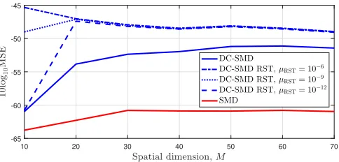
Fig. 4. Mean squared error versus spatial dimension M for SMD and DC-SMD with and without row-shift truncation for M ∈

{10; 20; 30; 40; 50; 60; 70} and µRST ∈ {10−6; 10−9; 10−12}.

D. Reconstruction Error

The ensemble-averaged mean squared reconstruction error was calculated for both algorithms, according to (13). For DC-SMD, this metric was recorded before and after the utilisation of row-shift truncation, to estimate the method’s impact. Fig. 4 shows the results for M ∈ {10; 20; 30; 40; 50; 60; 70}; from this, it is clear that the increased diagonalisation speed and lower cumulative complexity of DC-SMD come at the cost of a higher reconstruction error. To reduce this error, parameter

δ can be decreased; however, this will reduce the speed and increase the complexity of the algorithm, as more effort will be contributed to the divide step. Note that the relative difference in average MSE remains reasonably constant for increasing

M, and that the use of row-shift truncation results in a slightly higher reconstruction error for all dimensionalities.

The row-shift truncation step introduces further error by truncating small values from each row of F_{(z). This error}

can be decreased by using a smaller truncation parameter within the row-shift truncation step; however, this comes at the expense of a decreased reduction in paraunitary filter length. It can be observed that, for larger M, increasing µRST has little impact on the reconstruction error.

E. Paraunitary Filter Length

The ensemble-averaged paraunitary (PU) filter lengths were calculated for both algorithms. For DC-SMD, this metric was recorded before and after the utilisation of row-shift truncation,

10 20 30 40 50 60 70

Spatial dimension,M 50

100 150 200 250

P

U

L

en

g

th

DC-SMD

DC-SMD RST,µRST= 10−6

DC-SMD RST,µRST= 10−9 DC-SMD RST,µRST= 10−12 SMD

Fig. 5. Paraunitary filter length versus spatial dimension M for SMD and DC-SMD with and without row-shift truncation for M ∈

{10; 20; 30; 40; 50; 60; 70}and µRST ∈ {10−6; 10−9; 10−12}.

to estimate the method’s impact. Fig. 5 shows the results for

M ∈ {10; 20; 30; 40; 50; 60; 70}. It can be seen from this graph that the average paraunitary filter length is larger for DC-SMD than SMD for allM. The relative difference in average paraunitary filter length becomes larger for increasing

M; however, the use of row-shift truncation has successfully narrowed the gap.

IncreasingµRSTfor this method of truncation only slightly increased reconstruction error for largerM in Fig. 4; however, in Fig. 5, a significant decrease in paraunitary filter length is observed as µRSTis increased for M >10.

Note that — as in [16] — row-shift truncation was found to have minimal impact when applied to the paraunitary filters generated by SMD.

While larger paraunitary filters are disadvantageous for application purposes, the increased performance of DC-SMD in other areas may be of greater importance. In addition, for applications where a small change in reconstruction error is acceptable, increasing parameter µRST can offer significant filter length reduction.

V. CONCLUSION

In this paper, we have analysed the performance of a recently developed PEVD algorithm, DC-SMD, for parahermi-tian matrices of various spatial dimensionality. The parameter

M used to describe the dimensionality of such matrices can be directly related to the number of elements within a sensor array. Simulation results have demonstrated that DC-SMD offers significant complexity reduction over a traditional PEVD algorithm, SMD, when processing data analogous to that obtained from large sensor arrays. Furthermore, DC-SMD is able to provide substantially lower execution times than SMD; however, such benefits come with the disadvantage of increasing the mean squared reconstruction error and the paraunitary filter order.

When designing PEVD implementations for real applica-tions, the potential for the DC-SMD algorithm to increase diagonalisation performance while reducing complexity re-quirements offers benefits. A further advantage of the DC-SMD algorithm is its ability to produce multiple independent parahermitian matrices, which may be processed in parallel.

Given the results of this paper, it can be concluded that DC-SMD is suitable for broadband multichannel applications with a large number of sensors.

ACKNOWLEDGEMENT

Fraser Coutts is the recipient of a Caledonian Scholarship; we would like to thank the Carnegie Trust for their support.

This work was supported in parts by the Engineering and Physical Sciences Research Council (EPSRC) Grant number EP/K014307/1 and the MOD University Defence Research Collaboration in Signal Processing.

REFERENCES

[1] C. H. Ta and S. Weiss. A design of precoding and equalisation for broadband MIMO systems. InAsilomar SSC, pp. 1616–1620, Pacific Grove, CA, USA, Nov. 2007.

[2] P. P. Vaidyanathan. Multirate Systems and Filter Banks. Prentice Hall, Englewood Cliffs, 1993.

[3] S. Weiss, S. Bendoukha, A. Alzin, F. Coutts, I. Proudler, and J. Cham-bers. MVDR broadband beamforming using polynomial matrix tech-niques. InEUSIPCO, pp. 839–843, Nice, France, Sep. 2015. [4] A. Alzin, F. Coutts, J. Corr, S. Weiss, I. K. Proudler, and J. A. Chambers.

Adaptive broadband beamforming with arbitrary array geometry. In

IET/EURASIP ISP, London, UK, Dec. 2015.

[5] M. Alrmah, S. Weiss, and S. Lambotharan. An extension of the music algorithm to broadband scenarios using polynomial eigenvalue decom-position. In19th European Signal Processing Conference, pp. 629–633, Barcelona, Spain, Aug. 2011.

[6] S. Weiss, M. Alrmah, S. Lambotharan, J. McWhirter, and M. Kaveh. Broadband angle of arrival estimation methods in a polynomial matrix decomposition framework. InIEEE 5th Int. Workshop Comp. Advances in Multi-Sensor Adaptive Proc., St. Martin, pp. 109–112, Dec. 2013. [7] I. Gohberg, P. Lancaster, and L. Rodman.Matrix Polynomials. Academic

Press, New York, 1982.

[8] J. G. McWhirter, P. D. Baxter, T. Cooper, S. Redif, and J. Foster. An EVD Algorithm for Para-Hermitian Polynomial Matrices. IEEE TSP, 55(5):2158–2169, May 2007.

[9] S. Icart, P. Comon. Some properties of Laurent polynomial matrices. In

IMA Int. Conf. Math. Signal Proc., Birmingham, UK, Dec. 2012.

[10] P. Vaidyanathan. Theory of optimal orthonormal subband coders.IEEE TSP, 46(6):1528–1543, June 1998.

[11] S. Redif, S. Weiss, and J. McWhirter. Sequential matrix diagonalization algorithms for polynomial EVD of parahermitian matrices. IEEE TSP, 63(1):81–89, Jan. 2015.

[12] J. Corr, K. Thompson, S. Weiss, J. McWhirter, S. Redif, and I. Proudler. Multiple shift maximum element sequential matrix diagonalisation for parahermitian matrices. In IEEE Workshop on Statistical Signal Pro-cessing, pp. 312–315, Gold Coast, Australia, June 2014.

[13] Z. Wang, J. G. McWhirter, J. Corr, and S. Weiss. Multiple shift second order sequential best rotation algorithm for polynomial matrix EVD. In

EUSIPCO, pp. 844–848, Nice, France, Sep. 2015.

[14] J. Corr, K. Thompson, S. Weiss, J. G. McWhirter, and I. K. Proudler. Causality-Constrained multiple shift sequential matrix diagonalisation for parahermitian matrices. In EUSIPCO, pp. 1277–1281, Lisbon, Portugal, Sep. 2014.

[15] J. Corr, K. Thompson, S. Weiss, I. Proudler, and J. McWhirter. Row-shift corrected truncation of paraunitary matrices for PEVD algorithms. InEUSIPCO, pp. 849–853, Nice, France, Sep. 2015.

[16] J. Corr, K. Thompson, S. Weiss, I. Proudler, and J. McWhirter. Shortening of paraunitary matrices obtained by polynomial eigenvalue decomposition algorithms. InSSPD, pp. 1–5, Edinburgh, UK, Sep. 2015. [17] J. Foster, J. G. McWhirter, and J. Chambers. Limiting the order of poly-nomial matrices within the SBR2 algorithm. InIMA Int. Conf. Math. Sig-nal Proc., Cirencester, UK, Dec. 2006.

[18] C. H. Ta and S. Weiss. Shortening the order of paraunitary matrices in SBR2 algorithm. InICICSP, pp. 1–5, Singapore, Dec. 2007. [19] F. Coutts, J. Corr, K. Thompson, S. Weiss, J. Proudler, and J. McWhirter.

Memory and Complexity Reduction in Parahermitian Matrix Manipu-lations of PEVD Algorithms. InEUSIPCO, pp. 1633-1637, Budapest, Hungary, August 2016.

[20] F. Coutts, J. Corr, K. Thompson, S. Weiss, I. Proudler, and J. McWhirter. Complexity and Search Space Reduction in Cyclic-by-Row PEVD Algorithms. InAsilomar SSC, Pacific Grove, CA, Nov. 2016. [21] J. J. M. Cuppen. A divide and conquer method for the symmetric

tridiagonal eigenproblem.Num. Mathematik, 36(2):177–195, June 1980. [22] J. J. Dongarra and D. C. Sorensen. A fully parallel algorithm for the symmetric eigenvalue problem.SIAM JSSC, 8(2):139–154, March 1987. [23] D. Gill and E. Tadmor. An O(N2_{) method for computing the}

eigensystem of N×N symmetric tridiagonal matrices by the divide and conquer approach. SIAM JSSC, 11(1):161–173, Jan. 1990. [24] F. Coutts, J. Corr, K. Thompson, I. Proudler, and S. Weiss.

Divide-and-Conquer Sequential Matrix Diagonalisation for Parahermitian Matrices. Submitted toSSPD, London, UK, Dec. 2017.

[25] A. Jafarian and J. McWhirter. A novel method for multichannel spectral factorization. In EUSIPCO, pp. 1069–1073, Bucharest, Romania, Aug. 2012.