An examination of the benefits of factor investing in U.K. stock returns

(1)

Published by Canadian Center of Science and Education

An Examination of the Benefits of Factor Investing in U.K.

Stock Returns

Jonathan Fletcher1

1_{Strathclyde Business School, University of Strathclyde, Glasgow, United Kingdom}

Correspondence: Professor J. Fletcher, Department of Accounting and Finance, University of Strathclyde, Stenhouse Building, 199 Cathedral Street, Glasgow, G4 0QU, United Kingdom. Tel: 44-0-141-548-4963. E-mail: j.fletcher@strath.ac.uk

Received: January 20, 2018 Accepted: February 23, 2018 Online Published: March 15, 2018

doi:10.5539/ijef.v10n4p154 URL: https://doi.org/10.5539/ijef.v10n4p154

Abstract

This study uses the Bayesian approach of Wang (1998) to examine the benefits of factor investing in U.K. stock returns in the presence of market frictions. My study finds that factor investing provides significant performance benefits when the benchmark investment universe is the market index, even in the presence of market frictions such as portfolio constraints and trading costs. However when the benchmark investment universe includes industry portfolios, market frictions, such as no short selling constraints and trading costs, tends to eliminate the benefits of factor investing. Imposing less restrictive portfolio constraints, factor investing can generate significant performance for investors with higher risk aversion levels.

Keywords: factor investing, mean-variance analysis, Bayesian evaluation

1. Introduction

Linear factor models motivated by the capital asset pricing model (CAPM) and arbitrage pricing theory (APT) play a central role in practical applications such as evaluating the performance of managed funds, estimating expected excess returns (Sarisoy, Goeij, & Werker, 2017), and optimal portfolio choice (Uppal & Zaffaroni, 2017). A recent innovation in quantitative asset management has been the development of factor investing (Ang, 2014). The aim of factor investing is to allow investors to benefit from the risk premiums of different factors.

Empirical research in linear factor models has identified a number of different factors which are important in explaining cross-sectional stock returns. The most popular factors are based on the models of Fama and French (1993, 2015) and Carhart (1997) (Note 1), including size, value, momentum, profitability, and investment factors. These factors require long and short ends to exploit the factor risk premiums. The profitability of factor investing is captured by studies such as Eun, Lao, De Roon, and Zhang (2010), Israel and Moskowitz (2013) among others (Note 2).

A recent study by Briere and Szafarz (2017a) compare the performance of factor investing strategies of the size, value, profitability, investment, and momentum factors to an industry (sector) asset allocation strategy. Briere and Szafarz find that factor investing performs better when investors are able to short sell but sector investing performs better when there are no short selling constraints. Briere and Szafarz (2017b) find that combining factors and industries together leads to even better performance. The main advantage of sector investing lies in portfolio risk reduction and the main benefit of factor investing lies in higher expected return. Briere and Szafarz (2017c) explore further the role of short selling constraints in factor investing strategies. They find that imposing the Fama and French (1993) constraint (Note 3) on the factors actually leads to good performance and in some cases performs as well as the unconstrained mean-variance optimization.

(2)

optimal portfolio weights and proportional transaction costs. I also consider the impact of the less restrictive portfolio constraints used by Briere and Szafarz (2017c).

There are four main findings in my study. First, market frictions has a significant impact on the CER performance of the factor investing strategies. Second, when the benchmark investment universe is the market index, factor investing leads to a significant increase in CER performance even in the presence of market frictions. Third, when the benchmark investment universe includes the industry portfolios, market frictions tends to eliminate the incremental benefits of factor investing. Fourth, when investors face the more relaxed portfolio constraints of Briere and Szafarz (2017c), factor investing now delivers significant performance benefits to the benchmark investment universe including industry portfolios. My study suggests that market frictions has a significant impact on the performance benefits of factor investing.

My study makes two contributions to the literature. First, I complement the recent studies of Briere and Szafarz (2017a,b,c) by focusing on the U.K. market rather than the U.S. market. Recent studies by Hou, Xue, and Zhang (2017a) and Harvey (2017) highlight the importance of replication studies in Finance, which is common in other fields of science. I extend the Briere and Szafarz studies by considering the impact of trading costs and using the Bayesian approach rather than classical tests of mean-variance efficiency. Second, I extend the empirical evidence of linear factor models such as Fama and French (2015, 2016, 2017) in U.S. stock returns and Fletcher (2001), Gregory, Tharyan, and Christidis (2013), and Michou and Zhou (2016) among others in U.K. stock returns. I extend this evidence by focusing on the investment benefits of factor investing rather than evaluating the performance of the models.

My paper is organized as follows. Section 2 presents the research method. Section 3 describes the data used in my study. Section 4 reports the empirical results and the final section concludes.

2. Research Method

The mean-variance approach of Markowitz (1952), in the presence of a risk-free asset (Rf), assumes that investors select the optimal portfolio weights in N risky assets to:

Max x’u – (γ/2)x’Vx (1) where x is a (N,1) vector of optimal weights, u is a (N,1) vector of expected excess returns, V is the (N,N) covariance matrix, and γ is the level of risk aversion. The framework in equation (1) assumes that the investment in Rf is such that x’e + xRf = 1, where e is a (N,1) vector of ones and xRf is the weight in Rf. Equation (1) can also be estimated using portfolio constraints. In most of my analysis, I consider two models of constrained portfolio strategies. First, in the Constrained 1 portfolio strategies no short selling is allowed in the N risky assets (xi ≥ 0 for i=1,…,N) and in Rf (x’e ≤ 1). Second, in the Constrained 2 portfolio strategies, in addition to the short selling constraints, I add a 20% upper bound constraint(Note 4) in the N risky assets (xi ≤ 0.2 for i=1,….,N) (Note 5) for i = 1,…,N.

As well as considering the two constrained portfolio strategies, later in the paper, I examine the impact of using the more relaxed portfolio constraints on the factors implied the Fama & French (1993) model used by Briere and Szafarz (2017c). The size (SMB), value (HML), profitability (RMW), investment (CMA), and momentum (WML) factors in the Fama and French (1993, 2015), and Carhart (1997) assume a zero-cost constraint (Fama & French, 2017). The short end of the factor is set equal to the opposite sign and size of the long end of the factor. To impose this approach in the mean-variance optimization, I work with the zero-cost SMB, HML, RMW, CMA, and WML factors and impose the portfolio constraints on these factors. This approach implies that the short end of each factor is equal to the magnitude of the long end of the factor. As in Briere and Szafarz (2017c), either end of the each factor can be selected to be the long end in the optimization.

I use the mean-variance objective function in equation (1) to evaluate the performance of the optimal factor investing strategies. The performance measure is known as the Certainty Equivalent Return (CER) (Note 6). My main empirical results examine the increase in CER performance of adding the factors to a benchmark investment universe. Define K as the number of risky assets in the benchmark investment universe and N are the number of risky assets, which are added to the benchmark investment universe. The increase in CER performance (DCER) is given by:

DCER = (x’u – (γ/2)x’Vx) – (xb’u – (γ/2)xb’Vxb) (2)

(3)

I estimate the magnitude and test the statistical significance of the DCER measure using the Bayesian approach of Wang (1998). The Bayesion approach of Wang builds on the earlier work of Kandel, McCulloch, and Stambaugh (1995). An alternative approach to test either mean-variance intersection or spanning (Note 7) is developed by Gibbons, Ross, and Shanken (1989) and Huberman and Kandel (1987) for the unconstrained portfolio case. Classical tests of mean-variance intersection and spanning in the presence of portfolio constraints have been developed by Basak, Jagannathan, and Sun (2002), Briere, Drut, Mignon, Oosterlinck, and Szafarz (2013), and De Roon, Nijman, and Werker (2001) (Note 8). Li, Sarkar, and Wang (2003) point out that the Bayesian approach has a number of advantages over the classical approach. First, the Bayesian approach is a lot more easy to implement in the presence of portfolio constraints and can use a variety of performance measures. Second, the uncertainty in finite samples is incorporated into the posterior distribution. Third, the classical tests rely on a linear approximation to derive the standard errors of the mean-variance inefficiency measures, but the Bayesian approach uses the exact nonlinear function.

The Bayesian approach assumes that the N+K asset excess returns have a multivariate normal distribution (Note 9). I assume a non-informative prior about the expected excess returns u and the covariance matrix V. Define us and Vs as the sample moments of the expected excess returns and covariance matrix, and R as the (T,N+K) matrix of excess returns on the N+K assets. The posterior probability density function is given by:

p(u,V|R) = p(u|V,us,T)p(V|Vs,T) (3)

where p(u|V,us,T) is the conditional distribution of a multivariate normal (us, (1/T)V) distribution and p(V|Vs,T) is the marginal posterior distribution that has an inverse Wishart (TV, T-1) distribution (Zellner, 1971).

To approximate the posterior distribution of the DCER measure, I use the Monte Carlo method of Wang (1998). I use the following four-step approach. First, a random V matrix is drawn from an inverse Wishart (TVs,T-1) distribution. Second, a random u vector is drawn from a multivariate normal (us, (1/T)V) distribution. Third, given the u and V from steps 1 and 2, the DCER measure from equation (2) is estimated. Fourth, steps 1 to 3 are repeated 1,000 times to generate the approximate posterior distribution of the DCER measure.

The posterior distribution of the DCER measure is then used to assess the size of the performance benefits and the statistical significance of these benefits. The average value from the posterior distribution of the DCER measure provides the average performance benefits in terms of the increase in CER performance. The values of the 5th and 10th percentiles of the posterior distribution of the DCER measure provides a statistical test of the average DCER = 0 (Hodrick & Zhang, 2014). If the factors provide significant performance benefits, I expect to find a significant positive average DCER measure.

The Monte Carlo simulation also gives the approximate posterior distribution of the weights in the optimal portfolio strategies. Britten-Jones (1999) and Kan and Smith (2008) derive the sampling distribution of the optimal mean-variance portfolio weights when there are no portfolio constraints. The Bayesian approach provides an approximate posterior distribution of the optimal weights when there are portfolio constraints. I can use the posterior distribution to examine if the average weights in the optimal portfolios are more than two standard deviations from zero (Li et al., 2003).

The analysis so far ignores trading costs. I use the approach of Luttmer (1996) and De Roon et al. (2001) (Note 10) to incorporate the impact of trading costs of the performance of the strategies. I only consider this issue for the constrained portfolio strategies. Define tc = 1/ (1+ai), where ai is the proportional cost per transaction. Trading costs can be incorporated by adjusting the returns on the risky assets R (1+return) as tcR and then calculate the adjusted excess returns. The Bayesian approach is then used with the adjusted excess returns of the N+K risky assets. I consider two cases of trading costs. First, I set a cost per transaction at 50 basis points on all risky assets as in Balduzzi and Lynch (1999) and DeMiguel et al. (2009). Second, I assume cost per transaction of 50 basis points on the Losers and Winners factors but 10 basis points on all the other factors. I use higher trading costs on the Losers and Winners factors as these factors imply a much higher portfolio turnover (Frazzini, Israel, & Moskowitz, 2014; Novy-Marx & Velikov, 2016).

3. Data

(4)

LSPD and Thomson Financial Datastream, as the risk-free asset. Details on how the factor portfolios are constructed are included in the Appendix.

[image:4.595.74.529.211.398.2]

I examine the benefits of factor investing using two benchmark investment universes including the risk-free asset. The first is the U.K. market index. The second is ten U.K. industry portfolios. The industry portfolios include Resources, Basic Industries, General Industrials, Cyclical Consumer Goods, Noncyclical Consumer Goods, Retailers, Leisure and Media, Services, Financials, and Utilities. Details of the construction of the market index and industry portfolios are included in the Appendix. Table 1 reports summary statistics of the ten factor and ten industry portfolios and summary statistics of the correlations between the respective factor and industry portfolios, which includes the minimum, maximum, and average correlations.

Table 1. Summary statistics of factor portfolios and industry portfolios

Panel A:

Factors Mean Standard Deviation Industries Mean Standard Deviation

Big 0.454 4.288 Resource 0.583 6.002

Small 0.469 4.864 Basic industries 0.553 5.633

Growth 0.284 4.486 General industrials 0.519 5.616

Value 0.585 4.650 Cyclical consumer goods 0.466 6.564

Losers -0.043 5.723 Noncylical consumer goods 0.701 4.204

Winners 0.864 4.602 Retailers 0.350 4.700

Weak 0.391 4.597 Leisure and media 0.541 5.406

Robust 0.536 4.190 Services 0.395 5.568

Aggressive 0.244 4.905 Financials 0.420 5.678

Conservative 0.655 4.361 Utilities 0.478 5.518

Panel B:

Correlations Minimum Maximum Average

Factors 0.751 0.966 0.901

Industries 0.408 0.860 0.617

Note. The table reports summary statistics of 10 U.K. factor and industry portfolios between July 1983 and December 2016. The summary statistics in panel A include the mean and standard deviation of monthly excess returns (%). Panel B includes the minimum, maximum, and average correlations between the ten factor portfolios and ten industry portfolios respectively.

Panel A of Table 1 shows that there is a wide spread in the average excess returns across the ten factor portfolios. The mean excess returns range between -0.043% (Losers) and 0.864% (Winners). The Losers portfolio also has the highest volatility among the ten factors. The mean excess returns between the Big and Small factors are very close to each other, highlighting the negligible size effect over the sample period. The mean excess returns highlight the value, momentum, profitability and investment effects, where the mean excess return of the Value factor is higher than the Growth factor, the mean excess return of the Winners factor is higher than Losers factor, the mean excess return of the Robust factor is higher than Weak factor, and the mean excess return of the Conservative factor is higher than Aggressive factor. Among the five zero-cost factors, the momentum effect is the strongest by a wide margin. The ten factors are highly correlated with one another with an average correlation of 0.901. This pattern suggests that portfolio risk reduction benefits of investing in the factors is likely to be small. The correlation patterns are similar to Briere and Szafarz (2017a) in U.S. stock returns.

The industry portfolios have a narrower spread in the mean excess returns compared to the factor portfolios. The mean excess returns range between 0.350% (Retailers) and 0.701% (Noncyclical Consumer Goods). However the industry portfolios have a wider spread in volatility compared to the factor portfolios. The volatility of the industry portfolios range between 4.204% (Noncyclical Consumer Goods) and 6.564% (Cyclical Consumer Goods). The industry portfolios also have lower correlations compared to the factor portfolios. The average correlation for industry portfolios is 0.617 compared to 0.901 for the factor portfolios. and there is a wider range between the minimum and maximum correlations. This pattern suggests that portfolio risk reduction benefits are likely to be greater in the industry portfolios and is similar to Briere and Szafarz (2017a) in U.S. stock returns.

4. Empirical Results

(5)

[image:5.595.77.520.123.299.2]

strategies. Table 3 reports the mean and standard deviation of the posterior distribution of the optimal portfolio weights in the factor investing strategies.

Table 2. Performance of factor investing strategies

Panel A:

Unconstrained Mean Standard Deviation 5% 10% Median

γ=1 10.978 2.395 7.398 8.009 10.788

γ=3 3.659 0.798 2.466 2.669 3.596

γ=5 2.195 0.479 1.479 1.601 2.157

Panel B:

Constrained 1 Mean Standard Deviation 5% 10% Median

γ=1 0.762 0.241 0.379 0.465 0.762

γ=3 0.549 0.231 0.179 0.259 0.549

γ=5 0.374 0.190 0.107 0.155 0.351

Panel C:

γ=1 0.546 0.216 0.192 0.270 0.545

γ=3 0.380 0.185 0.118 0.159 0.360

γ=5 0.274 0.138 0.085 0.117 0.255

Note. The table reports summary statistics of the posterior distribution of the CER (%) performance of the optimal factor investing strategies between July 1983 and December 2016. The investment universe includes the excess returns of ten factor portfolios and the one-month U.K. Treasury Bill return. The summary statistics include the mean, standard deviation, fifth percentile (5%), tenth percentile (10%), and the median of the posterior distribution of the CER performance. Risk aversion (γ) levels are set equal to 1, 3, and 5. Panel A refers to the unconstrained portfolio strategies. Panel B refers to constrained portfolio strategies (Constrained 1), where no short selling is allowed in the ten factors and the one-month Treasury Bill. Panel C refers to constrained portfolio strategies (Constrained 2), where no short selling is allowed in the ten factors and the one-month Treasury Bill, and there is an upper bound constraint of 20% of each of the factors.

Table 3. Posterior distribution of the optimal factor investing portfolio weights

Panel A: Unconstrained Mean γ=1 Standard Deviation Mean γ=3 Standard Deviation Mean γ=5 Standard Deviation

Big -6.913 10.644 -2.304 3.548 -1.382 2.128

Small -8.113 11.287 -2.704 3.762 -1.622 2.257

Growth -11.466 6.784 -3.822 2.261 -2.293 1.356

Value 7.167 6.757 2.389 2.252 1.433 1.351

Losers -0.776 3.473 -0.258 1.157 -0.155 0.694

Winners 18.902 5.338 6.300 1.779 3.780 1.067

Weak -2.850 5.787 -0.950 1.929 -0.570 1.157

Robust 16.687 7.326 5.562 2.442 3.337 1.465

Aggressive -14.861 7.151 -4.953 2.383 -2.972 1.430

Conservative 7.457 7.200 2.485 2.400 1.491 1.440

Panel B: Constrained 1 Mean γ=1 Standard Deviation Mean γ=3 Standard Deviation Mean γ=5 Standard Deviation

Big 0 0 0.000 0.014 0.000 0.013

Small 0 0 0 0 0 0

Growth 0 0 0 0 0 0

Value 0.003 0.052 0.005 0.052 0.005 0.041

Losers 0 0 0 0 0 0

Winners 0.977 0.133 0.926 0.182 0.740 0.222

Weak 0 0 0 0 0 0

Robust 0 0 0.001 0.021 0.001 0.023

Aggressive 0 0 0 0 0 0

Conservative 0.016 0.117 0.030 0.135 0.034 0.122

Panel C: Constrained 2 Mean γ=1 Standard Deviation Mean γ=3 Standard Deviation Mean γ=5 Standard Deviation

Big 0.094 0.098 0.074 0.090 0.027 0.060

Small 0.094 0.098 0.046 0.078 0.009 0.034

[image:5.595.75.515.411.750.2]

(6)

Value 0.190 0.041 0.152 0.078 0.092 0.088

Losers 0 0 0 0 0 0

Winners 0.199 0.000 0.199 0.004 0.199 0.007

Weak 0.011 0.044 0.003 0.025 0.000 0.009

Robust 0.183 0.053 0.158 0.075 0.101 0.089

Aggressive 0 0 0 0 0 0

Conservative 0.198 0.016 0.193 0.031 0.181 0.051

Note. The table reports summary statistics of the posterior distribution of the optimal portfolio weights of the factor investing strategies between July 1983 and December 2016. The investment universe includes the excess returns of ten factor portfolios and the one-month U.K. Treasury Bill return. The summary statistics include the mean, and standard deviation from the posterior distribution of the optimal portfolio weights. Risk aversion (γ) levels are set equal to 1, 3, and 5. Panel A refers to the unconstrained portfolio strategies. Panel B refers to constrained portfolio strategies (Constrained 1), where no short selling is allowed in the ten factors and the one-month Treasury Bill. Panel C refers to constrained portfolio strategies (Constrained 2), where no short selling is allowed in the ten factors and the one-month Treasury Bill, and there is an upper bound constraint of 20% in each of the factors.

Panel A of Table 2 shows that there is a large significant positive CER performance for the unconstrained portfolio strategies. The average CER performance is highly significant at the 5% percentile. The median CER performance is close to the mean CER performance. The optimal portfolio weights underlying the large CER performance in panel A of Table 3 have extreme weights, with large long and short positions. Extreme weights are common in unconstrained sample mean-variance portfolios (Michaud, 1989). Increasing risk aversion levels leads to a substantial moderation in the mean and volatility of optimal weights. The large long positions are in the Winners, Robust, Conservative, and Value factors and the largest short positions are in the Growth, and Aggressive factors. The optimal weights in panel A of Table 3 also have substantial volatility. As a result, only the Winners, Robust, and Aggressive factors have mean weights more than two standard deviations from zero. The large volatility in portfolio weights is consistent with Britten-Jones (1999).

Imposing no short selling constraints in panel B of Table 2 leads to a large reduction in the mean and volatility of the CER performance. The reduction in volatility of CER performance is consistent with the lower estimation risk in sample mean-variance portfolios with no short selling constraints (Frost & Savarino, 1988; Jagannathan & Ma, 2003) (Note 11). The mean CER performance remains significant at the 5% percentile. Imposing no short selling constraints leads to a lack of diversification in the optimal factor investing portfolios as only the Winners factor is held in reasonable long positions in panel B of Table 3 with the remainder going to the riskless asset. The impact of no short selling constraints on the CER performance of the factor investing strategy is consistent with Briere and Szafarz (2017a,b,c). Briere and Szafarz show that factor investing strategies rely heavily on being able to short sell.

To ensure more diversification in the optimal factor investing strategies, imposing a 20% upper bound constraint leads to a further reduction in CER performance in panel C of Table 2. The CER performance remains significant at the 5% percentile. In the optimal portfolios, the dominant factors are Value, Winners, Robust, and Conservative. At γ = 5, it is only the Winners and Conservative factors with a positive mean weight more than two standard deviations from zero.

The analysis in Tables 2 and 3 ignores trading costs. I next examine the impact of trading costs on the performance of the factor investing strategies. I repeat the analysis in Table 2 for the constrained portfolio strategies using the two cases of trading costs. When trading costs are 50 basis points on all the factors, the significant positive CER performance of the constrained portfolio strategies disappears at the 5% percentile. When the trading costs are only 50 basis points on the Winners and Losers factors, there is a drop in the CER performance but the positive CER performance remains significant when the investor only faces short selling constraints. With the additional upper bound constraint, the significant positive CER performance disappears at the 5% percentile.

Tables 2 and 3 suggest that optimal factor investing strategies deliver significant positive CER performance and imposing portfolio constraints has a major impact of reducing CER performance. This result is similar to Briere and Szafarz (2017a,b,c). Adjusting for trading costs has a futher impact. This finding suggests that market frictions has a significant impact on the performance of the factor investing strategies. This finding is consistent with the impact of market frictions on other asset pricing applications such as He and Modest (1995), Luttmer (1996), De Roon et al. (2001), and De Roon and Szymanowsa (2012) among others.

(7)

[image:7.595.70.525.138.501.2]

is the market index (panel A) and the industry portfolios (panel B). To conserve space, I do not report the posterior distribution of the optimal portfolio weights but will discuss in the text (Note 12).

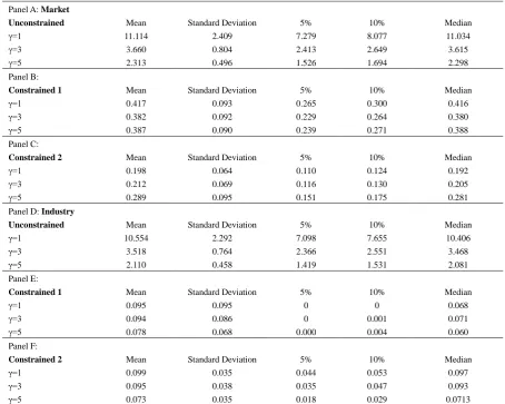
Table 4. Incremental CER performance of factor investing strategies relative to benchmark investment universe: market

Panel A: Market

γ=1 11.114 2.409 7.279 8.077 11.034

γ=3 3.660 0.804 2.413 2.649 3.615

γ=5 2.313 0.496 1.526 1.694 2.298

Panel B:

γ=1 0.417 0.093 0.265 0.300 0.416

γ=3 0.382 0.092 0.229 0.264 0.380

γ=5 0.387 0.090 0.239 0.271 0.388

Panel C:

γ=1 0.198 0.064 0.110 0.124 0.192

γ=3 0.212 0.069 0.116 0.130 0.205

γ=5 0.289 0.095 0.151 0.175 0.281

Panel D: Industry

γ=1 10.554 2.292 7.098 7.655 10.406

γ=3 3.518 0.764 2.366 2.551 3.468

γ=5 2.110 0.458 1.419 1.531 2.081

Panel E:

γ=1 0.095 0.095 0 0 0.068

γ=3 0.094 0.086 0 0.001 0.071

γ=5 0.078 0.068 0.000 0.004 0.060

Panel F:

γ=1 0.099 0.035 0.044 0.053 0.097

γ=3 0.095 0.038 0.035 0.047 0.093

γ=5 0.073 0.035 0.018 0.029 0.0713

Note. The table reports the summary statistics of the posterior distribution of the DCER (%) measure of adding ten factors to two benchmark investment universes between July 1983 and December 2016. The DCER measure is the increase in CER performance of adding the ten factors to the benchmark investment universe. The first benchmark universe is the excess returns of the market index (panel A). The second benchmark universe is the excess returns on ten industry portfolios and the one-month Treasury Bill return (panel B). The summary statistics include the mean, standard deviation, fifth percentile (5%), tenth percentile (10%, and median from the posterior distribution of the DCER measure. Risk aversion (γ) levels are set equal to 1, 3, and 5. The results are reported for the unconstrained portfolio strategies, constrained portfolio strategies (Constrained 1), where no short selling is allowed in the risky assets and one-month Treasury Bill, and the constrained portfolio strategies (Constrained 2), where in addition to the short selling constraints there is a 20% upper bound constraint in each risky asset.

Panel A of Table 4 shows that adding the ten factors to the benchmark investment universe of the market index leads to a significant increase in CER performance. The mean DCER measures are substantial for the unconstrained portfolio strategies and highly significant. The optimal portfolios underlying the increase in CER performance have extreme mean weights and are highly volatile. Imposing no short selling constraints leads to a substantial drop in the mean and volatility of the DCER measures and there is a further reduction with the upper bound constraints. However the benefits of factor investing remains significant as all the mean DCER measures are significant at the 5% percentile.

(8)

upper bound constraint, there is now a significant positive mean weights in the Value, Winners, Robust, and Conservative factors when γ = 1. Only the mean weights on the Winners and Conservative factors is significant across all levels of risk aversion. The Value and Robust factors are also significant at γ = 1. There is little exposure to the Market factor confirming again the performance benefits of factor investing even in the presence of portfolio constraints when the benchmark investment universe is the Market factor.

The results in panel A of Table 4 are consistent with Briere and Szafarz (2017b) who find that factor investing leads to both a significant increase in average returns and a significant reduction in volatility, even with no short selling constraints, relative to the market index. The results in panel A of Table 4 can also be interpreted in terms of the portfolio efficiency of the market index. The mean-variance efficiency of the market index is rejected here even in the presence of no short selling constraints. Portfolio constraints do however lead to a substantial reduction of the mean-variance inefficiency of the market index. This result is consistent with Wang (1998), Basak et al. (2002), Briere et al. (2013), and Fletcher (2017).

When the benchmark investment universe contains the industry portfolios in panel B of Table 4, adding the factors leads to a significant increase in CER performance for the unconstrained portfolio strategies. The mean DCER measures are substantial and of similar magnitude as in panel A of Table 4. The optimal weights underlying the increase in CER performance in the unconstrained portfolio strategies are extreme. The average weights on the factors are a lot more dominant than the average weights on the industry portfolios. The Winners and Robust factors have significant positive average. In contrast, only the Noncyclical Consumer Goods and Utilities industries have significant positive average weights. This pattern is consistent with the superior performance generated by the factor portfolios.

Imposing portfolio constraints largely eliminates the performance benefits of adding the factors to the benchmark investment universe of the industry portfolios. The mean DCER measures are small in economic terms. The mean DCER measures are not significant at the 5% percentile when only short selling constraints are imposed. The mean DCER measures are significant when the additional upper bound constraints are imposed. This result stems from the lower volatility of the DCER measure with the upper bound constraints.

With only no short selling constraints, the optimal portfolios are split between the Winners factor and Noncyclical Consumer Goods. However neither risky asset has a significant positive mean weight. The Winners factor still has the largest mean weight and ranges between 0.469 (γ = 5) and 0.655 (γ = 1). With the upper bound constraint, the industry portfolios dominate the optimal portfolios. Both the Winners factor and Noncyclical Consumer Goods have significant positive mean weights across all levels of risk aversion.

I next examine the impact of trading costs on the incremental CER performance of adding the factors to the two benchmark investment universes. I again focus only on the constrained portfolio strategies. Tables 5 and 6 reports the posterior distribution of the DCER measure for the two cases of trading costs when the benchmark investment universe is the market index (Table 5) and when the benchmark investment universe contains the industry portfolios (Table 6). Panel A of each table considers the case when trading costs are 50 basis points of all risky assets (Case 1). Panel B of each table considers the case when trading costs are 50 basis points on the Winners and Losers factors and 10 basis points on all the other risky assets.

Table 5. Incremental CER performance of factor investing in the presence of trading costs: benchmark investment universe is market index

Panel A: Case 1 TC

γ=1 0.429 0.094 0.271 0.313 0.427

γ=3 0.476 0.111 0.312 0.345 0.467

γ=5 0.602 0.138 0.396 0.438 0.583

γ=1 0.287 0.112 0.136 0.161 0.268

γ=3 0.417 0.144 0.205 0.246 0.403

γ=5 0.574 0.161 0.320 0.376 0.569

Panel B: Case 2 TC

γ=1 0.223 0.071 0.107 0.134 0.220

γ=3 0.228 0.077 0.107 0.133 0.228

[image:8.595.76.520.579.744.2]

(9)

γ=1 0.125 0.061 0.038 0.052 0.117

γ=3 0.164 0.086 0.052 0.070 0.147

γ=5 0.267 0.121 0.100 0.124 0.250

Note. The table reports summary statistics of the posterior distribution of the DCER (%) measure of adding ten factors to the benchmark investment universe adjusting for the impact of trading costs (TC) between July 1983 and December 2016. The DCER measure is the increase in CER performance of adding the ten factors to the benchmark investment universe. The benchmark universe is the excess returns of the market index. The summary statistics include the mean, standard deviation, fifth percentile (5%), tenth percentile (10%), and median from the posterior distribution of the DCER measure. The results are reported for the two constrained portfolio strategies. Constrained 1 portfolio strategies are where no short selling is allowed in the risky assets and the one-month Treasury Bill. Constrained 2 portfolio strategies are where in addition to no short selling constraints, there is a 20% upper bound constraint on each risky asset. There are two cases of trading costs. Panel A (Case 1 TC) refers to a cost per transaction in each risky asset of 50 basis points. Panel B (Case 2 TC) refers to a cost per transaction of 50 basis points in the Winners and Losers factors and 10 basis points in the other risky assets.

Table 6. Incremental CER performance of factor investing in the presence of trading costs: benchmark investment universe is industry portfolios

Panel A: Case 1 TC

γ=1 0.079 0.088 0 0 0.046

γ=3 0.052 0.062 0 0 0.030

γ=5 0.032 0.039 0 0 0.018

γ=1 0.052 0.039 0 0 0.048

γ=3 0.034 0.029 0 0 0.030

γ=5 0.024 0.024 0 0 0.019

γ=1 0.008 0.024 0 0 0

γ=3 0.013 0.027 0 0 0

γ=5 0.011 0.022 0 0 0.001

γ=1 0.043 0.028 0.001 0.008 0.040

γ=3 0.034 0.028 0 0.002 0.028

γ=5 0.020 0.021 0 0 0.015

Note. The table reports summary statistics of the posterior distribution of the DCER (%) measure of adding ten factors to the benchmark investment universe adjusting for the impact of trading costs (TC) between July 1983 and December 2016. The DCER measure is the increase in CER performance of adding the ten factors to the benchmark investment universe. The benchmark investment universe includes the excess returns on ten industry portfolios and the one-month Treasury Bill return. The summary statistics include the mean, standard deviation, fifth percentile (5%), tenth percentile (10%), and median from the posterior distribution of the DCER measure. Risk aversion (γ) levels are set equal to 1, 3, and 5. The results are reported for the constrained portfolio strategies. Constrained 1 portfolio strategies are where no short selling is allowed in the risky assets and the one-month Treasury Bill. Constrained 2 portfolio strategies are where in addition to no short selling constraints, there is a 20% upper bound constraint on each risky asset. There are two cases of trading costs. Panel A (Case 1 TC) refers to a cost per transaction in each risky asset of 50 basis points. Panel B (Case 2 TC) refers to a cost per transaction of 50 basis points in the Winners and Losers factors and 10 basis points in the other risky assets.

Panel A of Table 5 shows that when trading costs are 50 basis points on all risky assets, the benefits of factor investing actually increases when the benchmark investment universe is the market index. The mean DCER measures are larger than in panel A of Table 4, especially at higher levels of risk aversion. For both sets of constrained portfolio strategies, the mean DCER measures are large in economic terms and highly significant. The other interesting finding is that there is a positive relation between the DCER measure and the level of risk aversion. The optimal portfolios underlying the increase in CER performance have no exposure to the market index. A large part of the portfolio is now invested in the risk-free asset (Note 13) and the only factor to be held is the Winners factor.

[image:9.595.75.523.267.475.2]

(10)

level of risk aversion. Comparing to the results in panel A of Table 4, the differential trading costs leads to a substantive drop in performance when only the short selling constraints are imposed. There is less of an impact when the upper bound constraint is added. The optimal portfolios underlying the increase in CER performance are very different from panel A in Tables 4 and 5. There is now little exposure to the Winners factor. With only short selling constraints, the dominant factor is the Conservative factor. With the upper bound constraint, the dominant factors are the Conservative, Value, and Robust factors. In spite of the change in the composition of the optimal portfolios, there is still little exposure to the market index. This result is again consistent with the benefits of factor investing.

Table 6 shows that trading costs tends to eliminate the incremental CER performance of adding the factors to the benchmark investment universe of the industry portfolios. The mean DCER measures for the two groups of constrained portfolio strategies are all small and few are significant at the 5% and 10% percentiles. The optimal portfolios underlying the increase in CER performance, when trading costs are 50 basis points, the Winners factor dominates the industry portfolios when there are only short selling constraints. However, there is a large exposure to the risk-free asset. With the upper bound constraint, the combined weight of the industry portfolios exceeds the factor portfolios when γ = 1. With the differential trading costs, the optimal portfolios have only a small exposure to the factors and the industry portfolios dominate the factors.

[image:10.595.75.520.401.725.2]

Tables 5 and 6 show that the performance benefits of factor investing in the presence of market frictions only survives when the benchmark investment universe is the market index. The final issue I examine is whether using the more relaxed portfolio constraints of Briere and Szafarz (2017c) can restore the performance benefits of factor investing when the benchmark investment universe includes the industry portfolios. Table 7 reports the summary statistics of the posterior distribution of the DCER measure of adding the five zero-cost factors to the benchmark investment universe of the industry portfolios. Table 7 reports the posterior distribution of the DCER measures for the constrained portfolio strategies where there are no trading costs (panel A), and the two models of trading costs (panels B and C) (Note 14).

Table 7. Incremental CER performance of Zero-Cost factor investing: benchmark universe is industry portfolios

Panel A: No TC

γ=1 0.220 0.217 0 0 0.153

γ=3 0.302 0.197 0.036 0.068 0.268

γ=5 0.369 0.162 0.124 0.163 0.360

Constrained 2

γ=1 0.142 0.091 0.004 0.034 0.131

γ=3 0.235 0.086 0.086 0.118 0.240

γ=5 0.287 0.065 0.170 0.201 0.289

γ=1 0.197 0.188 0 0 0.143

γ=3 0.196 0.138 0.019 0.035 0.167

γ=5 0.158 0.109 0.017 0.035 0.138

γ=1 0.079 0.041 0.003 0.024 0.080

γ=3 0.082 0.037 0.018 0.031 0.083

γ=5 0.077 0.037 0.015 0.026 0.078

Panel C: Case 2 TC

γ=1 0.043 0.093 0 0 0

γ=3 0.108 0.105 0 0.001 0.078

γ=5 0.169 0.090 0.036 0.059 0.159

γ=1 0.071 0.071 0 0 0.050

γ=3 0.136 0.065 0.026 0.045 0.137

γ=5 0.166 0.050 0.087 0.101 0.164

(11)

increase in CER performance of adding the zero-cost factors to the benchmark investment universe. The benchmark investment universe includes the excess returns on ten industry portfolios and the one-month Treasury Bill return. The summary statistics include the mean, standard deviation, fifth percentile (5%), tenth percentile (10%), and median from the posterior distribution of the DCER measure. Risk aversion (γ) levels are set equal to 1, 3, and 5. There are two sets of constrained portfolio strategies. Constrained 1 is where no short selling is allowed in the risky assets and the one-month Treasury Bill. Constrained 2 is where in addition to the no short selling constraints, there is a 20% upper bound constraint oin each risky asset. The results are reported when there are no trading costs (TC) (panel A). Case 1 TC (panel B), there is a 50 basis points of cost per transaction on each risky asset. Case 2 TC (panel C) is when there is a 50 basis points cost per transaction on the WML factor and a 10 basis points cost per transaction in the other risky assets.

Table 7 shows that the performance of factor investing strategies improves with the more relaxed portfolio constraints. When there are no trading costs in panel A of Table 7, adding the five zero-cost factors to the benchmark investment universe tends to lead to a significant increase in CER performance. The exception to this result is when γ = 1 and only short selling constraints are imposed. The mean DCER measures are reasonably large in economic terms and significant at the 5% percentile. There is a positive relation between the DCER measure and the level of risk aversion. The performance benefits of factor investing stems from the WML factor. With only short selling constraints, the mean weight on the WML factor is 0.62 and above and is significant when γ = 3 and 5. With the upper bound constraints, the mean weight on the WML factor continues to be significant.

With trading costs of 50 basis points on all risky assets, there is a drop in the mean DCER measures for both constrained portfolio strategies. However with the exception of γ = 1 in the presence of short selling constraints, the mean DCER measures remain significant. The optimal portfolios underlying the increase in CER performance have a similar pattern to those when there are no portfolio constraints. The performance benefits of factor investing are again driven by the WML factor.

With differential trading costs in panel C of Table 7, the performance benefits of factor investing depends upon the level of risk aversion. When γ = 1, there are no performance benefits of factor investing for both constrained portfolio strategies. With only short selling constraints, there is a substantial drop in the mean DCER measure when γ = 1. At γ = 1, the mean weight on the WML factor is at its’ lowest. When γ =3, adding zero-cost factors to the benchmark investment universe only leads to a significant increase in CER performance when there is both short selling and upper bound constraints at the 5% percentile.

At the highest level of risk aversion, adding the zero-cost factors to the benchmark investment universe of the industry portfolios does lead to a significant increase in CER performance with the differential trading costs. The mean DCER measures for both the constrained portfolio strategies are significant at the 5% percentile. It is interesting to note that the mean DCER measures when γ = 5 is similar for the constrained portfolio strategies using the two cases of trading costs. With upper bound constraints, the mean DCER measure nearly doubles between the two cases of trading costs. The significant performance benefits of factor investing at γ = 5 is driven by the higher mean weight on WML factor. The performance benefits of using the more relaxed portfolio constraints is consistent with Briere and Szafarz (2017c).

5. Conclusions

This paper uses the Bayesian approach of Wang (1998) to examine the benefits of factor investing in U.K. stock returns in the presence of market frictions. There are four main findings in my study. First, when considering the factors on their own, factor investing leads to significant positive CER performance for both unconstrained and constrained portfolio strategies. This finding holds across all levels of risk aversion. Imposing portfolio constraints has a significant negative impact on the mean-variance performance of the factor investing strategies. This result is consistent with Briere and Szafarz (2017a,b,c) and the negative impact of short selling constraints on performance is consistent with Jacobs and Levy (1993) and Miller (2001). When trading costs are incorporated, much of the superior performance of the factor investing strategies disappear. This finding suggests that market frictions has a significant impact on the performance of the factor investing strategies.

(12)

who use different measures of mean-variance inefficiency than the one adopted in my study. From the perspective of testing the portfolio efficiency of the market index, this finding rejects the mean-variance efficiency of the market index even in the presence of portfolio constraints, which is consistent with Wang (1998), Li et al. (2003), Basak et al. (2002), Briere et al. (2013), and Fletcher (2017) among others.

Third, when the benchmark investment universe contains the industry portfolios, adding the factors to the benchmark investment universe leads to a large increase in CER performance for the unconstrained portfolio strategies. Imposing no short selling constraints eliminates the performance benefits of factor investing at the 5% percentile. This finding is consistent with Briere and Szafarz (2017a) who find factor investing strategies outperform industry strategies for unconstrained portfolio strategies by taking advantage of the factor premiums. There are significant performance benefits with the addition of the upper bound constraints but this result is due to the lower volatility of the DCER measures. Incorporating trading costs tends to eliminate the benefits of factor investing. In contrast, industry strategies perform better with constrained portfolio strategies by exploiting lower volatility. The finding that market frictions has a significant impact on the incremental CER performance of factor investing is consistent with the impact that market frictions has on other asset pricing applications such as He and Modest (1995), Luttmer (1996), De Roon et al. (2001), and De Roon and Szymanowska (2012) among others.

Fourth, factor investing can provide performance benefits to the benchmark investment universe of industry portfolios when the investor faces more relaxed portfolio constraints. This approach assumes that investors can actually invest in the short leg of the zero-cost factors by the same magnitude of the long leg. The performance benefits depend on the level of risk aversion. It is only when γ = 5, that there are significant increases in CER performance for both the constrained portfolio strategies even in the presence of trading costs. This superior performance is driven by the zero-cost WML factor. This finding is consistent with Briere and Szafarz (2017c).

My results suggest that the benefits of factor investing depends critically on the benchmark investment universe used in the presence of market frictions. When the benchmark investment universe includes the industry portfolios, the benefits of factor investing tend to disappear with portfolio constraints and trading costs unless the investor is able to invest in the short leg of the zero-cost factors. My study has examined the performance of factor investing across a given sample period and could be extended in a number of ways. First, exploring the benefits of factor investing across different economic states along the lines of Briere and Szafarz (2017a) or using the regime switching method of Ang and Bekaert (2004). Second, using a broader range of a different set of factors from newer factor models as Hou et al (2015), Stambaugh and Yuan (2017), Daniel et al. (2017), and Barillas, Kan, Robotti, and Shanken (2017). Third, examining the benefits of factor investing using small spread factors as Fama and French (2017). I leave these issues to future research.

References

Ang, A. (2014). Asset management a systematic approach to factor investing. Oxford University Press.

Ang, A., & Bekaert, G. (2004). How do regimes affect asset allocation? Financial Analysts Journal, 60, 86-99. https://doi.org/10.2469/faj.v60.n2.2612

Balduzzi, P., & Lynch, A. W. (1999). Transaction costs and predictability: Some utility cost calculations. Journal of Financial Economics, 52, 47-78. https://doi.org/10.1016/S0304-405X(99)00004-5

Barillas, F., Kan, R., Robotti, C., & Shanken, J. (2017). Model comparison with Sharpe ratios. Working Paper, University of Toronto.

Basak, G., Jagannathan, R., & Sun, G. (2002). A direct test for the mean-variance efficiency of a portfolio.

Journal of Economic Dynamics and Control, 26, 1195-1215.

https://doi.org/10.1016/S0165-1889(01)00044-6

Best, M. J. (2010). Portfolio optimization. CRC Press.

Best, M. J., & Grauer, R. R. (1990). The efficient set mathematics when the mean variance problem is subject to general linear constraints. Journal of Economics and Business, 42, 105-120. https://doi.org/10.1016/1057-5219(92)90012-S

Best, M. J., & Grauer, R. R. (2011). Prospect-theory portfolios versus power-utility and mean-variance portfolios. Working Paper, University of Waterloo.

Briere, M., & Szafarz, A. (2017a). Factor investing: Risk premia vs. diversification benefits. Working Paper, Paris Dauphine University.

(13)

Paris Dauphine University.

Briere, M., & Szafarz, A. (2017c). Factor investing: The rocky road from long-only to long-short. In E. Jurczenko (Ed), Factor Investing. Elsevier, forthcoming.

Briere, M., Drut, B., Mignon, V., Oosterlinck, K., & Szafarz, A. (2013). Is the market portfolio efficient? A new test of mean-variance efficiency when all assets are risky. Finance, 34, 7-41.

Britten-Jones, M. (1999). The sampling error in estimates of mean-variance efficient portfolio weights. Journal of Finance, 54, 655-671. http://dx.doi.org/10.1111/0022-1082.00120

Carhart, M. M. (1997). Persistence in mutual fund performance. Journal of Finance, 52, 57-82. http://dx.doi.org/10.1111/j.1540-6261.1997.tb03808.x

Cazalet, Z., & Roncalli, T. (2014). Facts and fantasies about factor investing. Working Paper, Amundi Asset Management.

Daniel, K., Hirshleifer, D., & Sun, L. (2017). Short- and long-horizon behavioral factors. Working Paper, Columbia University.

De Roon, F. A., & Karehnke, P. (2017). Spanning tests for assets with option-like payoffs: The case of hedge funds. Working Paper, University of New South Wales.

De Roon, F. A., & Szymanowska, M. (2012). Asset pricing restrictions on predictability: Frictions matter. Management Science, 58, 1916-1932. http://dx.doi.org/10.1287/mnsc.1120.1522

De Roon, F. A., Nijman, T. E., & Werker, B. J. M. (2001). Testing for mean-variance spanning with short sales constraints and transaction costs: The case of emerging markets. Journal of Finance, 56, 721-742. http://dx.doi.org/10.1111/0022-1082.00343

DeMiguel, V., Garlappi, L., & Uppal, R. (2009). Optimal versus naïve diversification: How inefficient is the 1/N strategy? Review of Financial Studies, 22, 1915-1953. https://doi.org/10.1093/rfs/hhm075

Dimson, P., & Marsh, P. R. (2001). U.K. financial market returns 1955-2000. Journal of Business, 74, 1-31. http://dx.doi.org/10.1086/209661

Dimson, P., Nagel, S., & Quigley, G. (2003). Capturing the value premium in the U.K. 1955-2001. Financial Analysts Journal, 59, 35-45. https://doi.org/10.2469/faj.v59.n6.2573

Eun, C. S., Lai, S., De Roon, F. A., & Zhang, Z. (2010). International diversification with factor funds. Management Science, 56, 1500-1518. https://doi.org/10.1287/mnsc.1100.1191

Fama, E. F., & French, K. R. (1993). Common risk factors in the returns on stocks and bonds. Journal of Financial Economics, 33, 3-56. https://doi.org/10.1016/0304-405X(93)90023-5

Fama, E. F., & French, K. R. (2012). Size, value, and momentum in international stock returns. Journal of Financial Economics, 105, 457-472. https://doi.org/10.1016/j.jfineco.2012.05.011

Fama, E. F., & French, K. R. (2015). A five-factor asset pricing model. Journal of Financial Economics, 116, 1-22. https://doi.org/10.1016/j.jfineco.2014.10.010

Fama, E. F., & French, K. R. (2016). Dissecting anomalies with a five-factor model. Review of Financial Studies, 29, 69-103. https://doi.org/10.1093/rfs/hhv043

Fama, E. F., & French, K. R. (2017). Choosing factors. Working Paper, University of Chicago.

Fletcher, J. (2001). An examination of alternative factor models in UK stock return. Review of Quantitative Finance and Accounting, 16, 117-130. https://doi.org/10.1023/A:1011270907471

Fletcher, J. (2017). Can short selling constraints explain the portfolio inefficiency of U.K. benchmark model. Advances in Investment Analysis and Portfolio Management, forthcoming.

Frazzini, A., Israel, R., & Moskowitz, T. (2014). Trading costs of asset pricing anomalies. Working Paper, University of Chicago.

Frost, P. A., & Savarino, J. E. (1988). For better performance: Constrain portfolio weights. Journal of Portfolio Management, 15, 29-34. https://doi.org/10.3905/jpm.1988.409181

Gibbons, M. R., Ross, S. A., & Shanken, J. (1989). A test of the efficiency of a given portfolio. Econometrica, 57, 1121-1152. http://dx.doi.org/10.2307/1913625

(14)

implementing dynamic investment strategies: A comparison of the returns and investment policies. Management Science, 39, 856-871. http://dx.doi.org/10.1287/mnsc.39.7.856

Gregory, A., Tharyan, R., & Christidis, A. (2013). Constructing and testing alternative versions of the Fama-French and Carhart models in the UK. Journal of Business Finance and Accounting, 40, 172-214. http://dx.doi.org/10.1111/jbfa.12006

Hansen, L. P., & Jagannathan, R. (1991). Implications of security market data for models of dynamic economies. Journal of Political Economy, 99, 225-262. http://dx.doi.org/10.1086/261749

Hansen, L. P., Heaton, J., & Luttmer, E. G. J. (1995). Econometric evaluation of asset pricing models. Review of Financial Studies, 8, 237-274. https://doi.org/10.1093/rfs/8.2.237

Harvey, C. R. (2017). The scientific outlook in financial economics. Journal of Finance, 72, 1399-1440. http://dx.doi.org/10.1111/jofi.12530

He, H., & Modest, D. M. (1995). Market frictions and consumption-based asset pricing. Journal of Political Economy, 103, 94-117. http://dx.doi.org/10.1086/261977

Hodrick, R. J., & Zhang, X. (2014). International diversification revisited. Working Paper, University of Columbia.

Hou, K., Xue, C., & Zhang, L. (2015). Digesting anomalies: An investment approach. Review of Financial Studies, 28, 650-705. https://doi.org/10.1093/rfs/hhu068

Hou, K., Xue, C., & Zhang, L. (2017a). Replicating anomalies. Working Paper, Ohio State University.

Hou, K., Xue, C., & Zhang, L. (2017b). A comparison of new factor models. Working Paper, Ohio State University.

Huberman, G., & Kandel, S. (1987). Mean-variance spanning. Journal of Finance, 42, 873-888. http://dx.doi.org/10.1111/j.1540-6261.1987.tb03917.x

Israel, R., & Moskowitz, T. (2013). The role of shorting, firm size, and time on market anomalies. Journal of Financial Economics, 108, 275-301. https://doi.org/10.1016/j.jfineco.2012.11.005

Jacobs, B. I., & Levy, K. N. (1993). Long short equity investing. Journal of Portfolio Management, 20, 52-64. https://doi.org/10.3905/jpm.1993.52

Jagannathan, R., & Ma, T. (2003). Risk reduction in large portfolios: Why imposing the wrong constraint helps. Journal of Finance, 58, 1651-1683. http://dx.doi.org/10.1111/1540-6261.00580

Kan, R., & Smith, D.R. (2008). The distribution of the sample minimum-variance frontier. Management Science, 54, 1364-1380. https://doi.org/10.1287/mnsc.1070.0852

Kan, R., & Zhou, G. (2012). Tests of mean-variance spanning. Annals of Economics and Finance, 13, 145-193.

Kan, R., Wang, X., & Zhou, G. (2017). On the value of portfolio optimization under estimation risk: The case without risk-free asset. Working Paper, University of Toronto.

Kandel, S., McCulloch, R., & Stambaugh, R. F. (1995). Bayesian inference and portfolio efficiency. Review of Financial Studies, 8, 1-53. https://doi.org/10.1093/rfs/8.1.1

Kirby, C., & Ostdiek, B. (2012). It’s all in the timing: Simple active portfolio strategies that outperform naïve diversification. Journal of Financial and Quantitative Analysis, 47, 437-467. https://doi.org/10.1017/S0022109012000117

Kroll, Y., Levy, H., & Markowitz, H. (1984). Mean-variance versus direct utility maximization. Journal of Finance, 39, 47-61. http://dx.doi.org/10.1111/j.1540-6261.1984.tb03859.x

Li, K., Sarkar, A., & Wang, Z. (2003). Diversification benefits of emerging markets subject to portfolio constraints. Journal of Empirical Finance, 10, 57-80. https://doi.org/10.1016/S0927-5398(02)00027-0

Liu, W., & Strong, N. (2008). Biases in decomposing holding period portfolio returns. Review of Financial Studies, 21, 2243-2274. https://doi.org/10.1093/rfs/hhl034

Luttmer, E. G. J. (1996). Asset pricing in economies with frictions. Econometrica, 64, 1439-1467. http://dx.doi.org/10.2307/2171838

Markowitz, H. (1952). Portfolio selection. Journal of Finance, 7, 77-91. http://dx.doi.org/10.1111/j.1540-6261.1952.tb01525.x

(15)

Quantitative Analysis, 7, 1851-1872. https:/doi.org/10.2307/2329621

Michaud, R. O. (1989). The Markowitz optimization enigma: Is ‘optimized’ optimal. Financial Analysts Journal, 45, 31-42. https://doi.org/10.2469/faj.v45.n1.31

Michou, M., & Zhou, H. (2016). On the information content of new asset pricing factors in the UK. Working Paper, University of Edinburgh.

Miller, E. M. (2001). Why the low returns to beta and other forms of risk. Journal of Portfolio Management, 27, 40-56. https://doi.org/10.3905/jpm.2001.319791

Novy-Marx, R., & Velikov, M. (2016). A taxonomy of anomalies and their trading costs. Review of Financial Studies, 29, 104-147. https://doi.org/10.1093/rfs/hhv063

Roll, R. (1977). A critique of the asset pricing theory’s tests Part I: On past and potential testability of the theory. Journal of Financial Economics, 4, 129-176. https://doi.org/10.1016/0304-405X(77)90009-5

Sarisoy, C., de Goeij, P., & Werker, B. J. M. (2017). Linear factor models and the estimation of expected returns. Academic Paper, Netspar.

Shumway, T. (1997). The delisting bias in CRSP data. Journal of Finance, 52, 327-340. http://dx.doi.org/10.1111/j.1540-6261.1997.tb03818.x

Stambaugh, R. F., & Yuan, Y. (2017). Mispricing factors. Review of Financial Studies, 30, 1270-1315. https://doi.org/10.1093/rfs/hhw107

Sun, L., Wei, K. C. J., & Xie, F. (2014). On the explanations of the gross profitability effect: Insights from international equity markets. Working Paper, Hong Kong University of Science and Technology.

Tu, J., & Zhou, G. (2011). Markowitz meets Talmud: A combination of sophisticated and naïve diversification strategies. Journal of Financial Economics, 99, 204-215. https://doi.org/10.1016/j.jfineco.2010.08.013

Uppal, R., & Zaffaroni, P. (2017). Portfolio choice with model misspecification: A foundation for alpha and beta portfolios. Working Paper, EDHEC.

Wang, Z. (1998). Efficiency loss and constraints on portfolio holdings. Journal of Financial Economics, 48, 359-375. https://doi.org/10.1016/S0304-405X(98)00015-4

Zellner, A. (1971). An introduction to Bayesian inference in econometrics. Wiley, New York.

Notes

Note 1. A new range of factor models have been recently proposed by Hou, Xue, and Zhang (2015,2017a,b), Stambaugh and Yuan (2017), and Daniel, Hirshliefer & Sun (2017) among others.

Note 2. Cazalet and Roncalli (2014) provide an excellent review of issues in factor investing.

Note 3. This zero-cost constraint enforces that the short leg of each factor has the opposite sign and same weight as the long leg.

Note 4. The upper bound constraint enforces a degree of diversification in the optimal portfolio since no short selling often results in a portfolio with a small number of long positions.

Note 5. See Merton (1972), Roll (1977), Best and Grauer (1990) for the mathematics of the mean-variance frontier. Best (2010) provides a textbook treatment of the mathematics and the quadratic programming solutions to the mean-variance frontier.

Note 6. The CER performance is used in a number of empirical studies of optimal portfolio choice including DeMiguel, Garlappi, and Uppal (2009), Tu and Zhou (2011), and Kan, Wang, and Zhou (2017) among others.

Note 7. Mean-variance intersection between two mean-variance frontiers occurs when the two frontiers intersect at only one point. Mean-variance spanning occurs when the two frontiers coincide. Kan and Zhou (2012) provide a review of mean-variance spanning tests when the only portfolio constraint is the budget constraint.

Note 8. De Roon and Karahnke (2017) develop tests of mean-variance-skewness spanning, which is relevant when the risky assets have option-like payoffs, such as hedge funds.

(16)

Note 10. See also He and Modest (1995) and Hansen, Heaton, and Luttmer (1995). A number of studies show that market frictions has a significant impact on different asset pricing applications such as the Hansen and Jagannathan (1991) volatility bounds (He & Modest, 1995; Luttmer, 1996), diversification benefits of emerging markets (De Roon et al., 2001), and stock return predictability and asset pricing models (De Roon & Szymanowska, 2012).

Note 11. Basak et al. (2002) find that the standard error of their mean-variance inefficiency measure increases with the no short selling constraints. They attribute this to the fact that their classical test of mean-variance efficiency relies on a linear approximation which becomes more unreliable when there are short selling constraints.

Note 12. Results are available on request.

Note 13. Kan et al. (2017) show that the poor performance of the sample mean-variance portfolio in DeMiguel et al. (2009) partly stems from the holding of the tangency portfolio. Allowing for an investment in the risk-free asset leads to a substantial improvement in performance. See also Kirby and Ostdiek (2012).

Note 14. To implement the trading costs for zero-cost factors, I follow the approach of Eun et al. (2010) and subtract the cost per transaction from the excess returns of the zero-cost factors.

Note 15. Investment trusts are closed-end funds.

Appendix

1) Factor Portfolios

I form the factor portfolios using the long and short legs of the factors in the Fama and French (2015) and Carhart (1997) models. To form the Value and Growth factors, I use a similar approach to Fama and French (2012). At the start of July each year between 1983 and 2016, all stocks on LSPD are ranked independently by their market value at the end of June and the book-to-market (BM) ratio from the prior calendar year. The BM ratio is calculated using the book value of equity at the fiscal year-end (WC03501) during the previous calendar year from Worldscope and the year-end market value. Stocks are grouped into two size categories (Small and Big), where the Small group are the companies in the bottom 10% of aggregate market capitalization and the Big group are the companies in the largest 90% of aggregate market capitalization. Stocks are also grouped into three BM groups (Growth, Neutral, and Value) using breakpoints of 30% and 70% of the BM ratio of Big stocks. Six size/BM portfolios (SG, SN, SV, BG, BN, BV) are formed using the intersection of the size and BM groups. I exclude companies with negative book values and zero market values. I then calculate monthly buy and hold portfolio returns for the next year, where the initial weights are value weighted by the market value of the companies at the end of June.

I make some corrections which are followed across all portfolios. I exclude stocks which are investment trusts (Note 15), secondary shares, and foreign companies. If a company in a portfolio dies or has a temporary suspension, then the missing returns are coded to zero as in Liu and Strong (2008). I correct for the delisting bias of Shumway (1997) as in Dimson, Nagel, and Quigley (2003) by converting the final return on the death event date to -100%, where LSPD deems the company’s death valueless.

From the six size/BM portfolios, I form two size factors, and a Value and Growth factor. The size factors are a small stock factor (SmallBM) and a large stock factor (BigBM). The SmallBM factor is given by the mean return of the SG, SN, and SV portfolios. The BigBM factor is given by the mean return of the BG, BN, and BV portfolios. The Value factor is given by the average returns of the SV and BV portfolios. The Growth factor is given by the average returns of the SG and BG portfolios.