A three-dimensional modeling for coalescence of multiple cavitation bubbles near a rigid wall

1

A three-dimensional modelling for coalescence of multiple cavitation

bubbles near a rigid wall

Rui Han (韩蕊)1,2_{, Longbin Tao} 1,2*_{, A-Man Zhang (张阿漫)} 1_{,Shuai Li (李帅)} 1

1) College of Shipbuilding Engineering, Harbin Engineering University, Harbin 150001, China

2) Department of Naval Architecture, Ocean and Marine Engineering, University of Strathclyde, Glasgow G4 0LZ, United Kingdom

Abstract: Boundary Integral Method (BIM) has been widely and successfully applied to cavitation bubble dynamics, however, the physical complexities involved in the coalescence of multiple bubbles are still challenging for numerical modelling. In this study, an improved three-dimensional (3D) BIM model is developed to simulate the coalescence of multiple cavitation bubbles near a rigid wall, including an extreme situation when cavitation bubbles are in contact with the rigid wall. As the first highlight of the present model, a universal topological treatment for arbitrary coalescence is proposed for 3D cases, combined with a density potential method and an adaptive remesh scheme to maintain a stable and high-accuracy calculation. Modelling for the multiple bubbles attached to the rigid boundary is the second challenging task of the present study. The effects of the rigid wall are modelled using the method of image, thus the boundary value problem is transformed to the coalescence of real bubbles and their images across the boundary. Additionally, the numerical difficulties associated with the splitting of a toroidal bubble and self-coalescence due to the self-film-thinning process of a coalesced bubble are successfully overcome. The present 3D model is verified through convergence studies and further validated by the purposely conducted experiments. Finally, representative simulations are carried out to elucidate the main features of a coalesced bubble near a rigid boundary and the flow fields are provided to reveal the underlying physical mechanisms.

2

I.

INTRODUCTION

For a cavitation bubble near a rigid wall, the high-speed liquid jet towards the boundary and the shock wave emission during the final collapse phase of the bubble are responsible for cavitation erosion and structural damages 1-7_{. In practical situations, there exist a large number of cavitation}

bubbles in the flow, thus the bubble collapse pattern and jetting behaviour are strongly influenced by not only the structure but also nearby bubbles 8-11_{. Researches on multi-bubble interaction near a rigid}

wall have great significance for various applications including cavitation erosion 3, 12_{, ultrasonic}

cleaning 13, 14_{, seabed exploration} 15_{, and biomedical applications} 16_.

As the most fundamental problem and the basic unit of bubble clusters, two-bubble system has been studied and reported in literatures. The effects of inter-bubble distance, size difference and generation time on dynamics of two bubbles in the free field were experimentally investigated and different bubble collapse patterns were observed17, 18_{. When a rigid boundary is inserted, the collapse}

pattern and jet direction of the two bubbles are inevitably changed. Chew et al19_{conducted a series of}

experiments to study the interaction between two bubbles arranged in a horizontal line and a rigid wall. The authors presented a graph predicting the direction of the water jets due to the combined effect of another bubble and the rigid wall. As the inter-bubble distance decreases, their mutual interaction will become stronger and coalescence of two bubbles may occur when the inter-bubble distance is sufficiently small. So far, there have been a few studies on the coalescence of two cavitation bubbles. Since the film thinning process before coalescence is inertia dominated 20_{, the boundary integral}

method (BIM) has been successfully used to simulate the coalescence of two explosion bubbles with high Reynolds numbers 21,22_{. Han et al} 23 _{numerically investigated the coalescence and collapse of}

bubble pairs near a rigid wall using an axisymmetric BIM model. It was found that a weakened pressure wave was emitted in the weak and intermediate interactions due to the splitting of the collapsing coalesced bubble in a toroidal form. Therefore, considerable attention is devoted to modelling the bubbles that are very close to or in contact with a rigid boundary, which is more crucial to cavitation erosion and other applications3,24-27_.

The axisymmetric configuration of two bubbles near a rigid wall is a specific situation 8, 23 _{and an}

3

modelling. Numerous studies have been conducted on single bubble dynamics under different boundary conditions using 3D BIM 28-35_{. However, the complex topological treatment during bubble}

coalescence renders the development of a 3D model difficult. Besides, many gas nuclei in the flow are often very close or even attached to a rigid wall, and the close proximity leads to large deformation and distortion of bubble surface, and even singularity problems, which are general challenges in BI simulations32,36_{. In previous studies, the distance between the bubble surface and the nearby boundary}

is controlled to a minimum value that is no less than the mesh size32,36,37_{. This crude treatment works}

well if the dimensionless distance (scaled by the maximum bubble radius) between the bubble centre and the boundary is larger than 0.5. However, a situation with smaller distance requires a more robust and reliable method. Given this, the first aim of this study is to develop a robust 3D model for arbitrary coalescence of multiple cavitation bubbles. A universal topological treatment for arbitrary coalescence is proposed. A density potential method 22, 38 _{is adopted to obtain an adaptive non-uniform mesh}

distribution for higher accuracy, in which a density potential function related to the coalescence is put forward. Besides, a weighted moving least-square smoother is applied to eliminate the instabilities in the simulation. A simple but robust remesh scheme is used to avoid the mesh distortion during the highly non-spherical bubble evolution and to ensure the mesh quality. As for the simulation of the coalesced bubble in contact with the rigid wall (defined as ‘contact cases’), an image method is introduced to transform the problem to the coalescence of real bubbles and their images across the boundary, which can then be solved with the robust topological treatment developed in the present study.

After the jet impacts on the opposite face of the bubble, a toroidal bubble is formed, indicating the transition of the flow domain from a singly connected to a doubly connected form. The modelling of 3D toroidal bubble dynamics has been a challenging problem for a long time due to physical and numerical instabilities 30, 38_{. To date, very few studies have been reported focusing on 3D toroidal}

bubble dynamics. Therefore, to address this gap, an exact approach has been proposed to examine the dynamic behaviours of a coalesced bubble in the toroidal phase.

4

to maintain the stability and accuracy of the three-dimensional calculation. The convergence and the validity of the present 3D model are proved by comparisons with the axisymmetric model and two experiments, respectively. Based on the numerical simulation, further results and discussions on the complex phenomena in multi-bubble coalescence are presented in Section IV.Finally, conclusions and outlook are given in Section V.

II.

PHYSICAL PROBLEM AND MATHEMATICAL MODEL

A. Description of the physical problem

Consider two cavitation bubbles above a rigid wall, as shown in FIG. 1. The cavitation bubble far away from the rigid wall is referred to as bubble 1; while in a horizontal configuration, the left bubble is referred to as bubble 1 and the other one is bubble 2. A Cartesian coordinate system O-xyz is adopted in the following modelling and discussion. The origin of the coordinate system is placed at the initial centre of bubble 1 and the z-axis points in the opposite direction of gravity. The definitions of some parameters are also given in FIG. 1. The distance between the rigid wall and the initial centres of cavitation bubbles are denoted by dbw1 and dbw2, respectively, the distance between the centres of two bubbles at the initiation moment is denoted by dbb and the maximum equivalent radii of the two bubbles

5

FIG. 1. Schematic view of the coordinate system and the arrangement of two cavitation bubbles above a rigid wall in (a) non-contact cases and (b) contact cases, respectively.

B. Boundary Integral Method

For the physical problem in the present study, the Reynolds number (defined as Re = URmax/ν, where Uis the mean velocity on the bubble wall, Rmax is the maximum equivalent bubble radius, and

ν is the kinematic viscosity of the fluid) and the Weber number (defined as We = ρU2_R

max/σ, where σ is the coefficient of surface tension) associated with the experiments can be estimated as O(105_{) and}

O(104_{), respectively. Therefore, the viscosity and surface tension are negligible in such transient} process and the BIM based on the potential flow theory is used to simulate the coalescence of two bubbles near a rigid wall.

In the framework of the potential flow theory, the fluid surrounding the cavitation bubbles is assumed inviscid, incompressible and the flow is irrotational. These assumptions stand well at least during the first cycle of cavitation bubbles, which have been confirmed by many previous studies 33,

39-43_{. Thus the velocity potential φ can be introduced in the mathematical model that satisfies the}

Laplace equation and the boundary integral equation

1 2

2 _{=0, ( ) ( )} ( ) _{( ) ( ),}

b b

S S

G

c G dS

n n



  



 

 

  _  _

 

 



p p q q (1)

6

as G1 p q 1 p q ' with q' being the reflected image of q across the boundary.

In this study, the heat transfer is ignored in the whole process 39, 40, 44_{, the internal pressure of a}

cavitation bubble P is thus related to the bubble initial state (P0 and V0) and its volume (V), yielding

0 0 , V P P V   

  _{ } (2)

where λ is the ratio of the specific heat for the gas and λ = 1.25 in this study.

The dynamic and kinematic boundary conditions on bubble surfaces can be written as 2 d , d 2 P P gz t      

   (3)

d

, dt  

r

(4)

where P∞ is the ambient pressure on the plane of the centre of cavitation bubble 1 at inception, ρ is the fluid density and g is the acceleration of gravity.

In the present study, it is assumed that the internal gases reach equilibrium instantaneously after coalescence, indicating that the effect of the changes in the bubble pressure on the external liquid flow is ignored 21, 22_{. The internal energy of the system before and after the coalescence remains the same}

without energy loss 21, 22_,





where n1 and n2 are the amount of moles of gases in bubbles 1 and 2, respectively, cv is the heat capacity at constant volume of the gas, T is the temperature of the coalesced bubble and T1 and T2 are the temperatures of the bubbles before coalescence. In the whole process, the internal gas of the bubble behaves according to the ideal gas law, yielding 21, 22





1 1 1 1

2 2 2 2 , ,

,

P V n n T

PV n T PV n T

  

   

c0 c0

(6)

where Pc0 and Vc0 are the initial pressure and volume of the coalesced bubble, respectively and ℜ is the universal gas constant. From equations (5) and (6), we can obtain 21, 22

1 1 2 2.

P Vc0 c0 PV PV (7)

7

neglected (within 3% for all coalescence cases), i.e. the initial volume of the coalesced bubble equals the total volume of bubbles 1 and 2 21, 22_{, the initial pressure of the coalesced bubble is}



 



Pc0  PV PV V V (8)

Then the subsequent pressure of the coalesced bubble can be calculated using equation (2).

C. Initial conditions and nondimensionalization

The initial parameters are deduced based on the oscillation of a spherical bubble in an infinite field (Rayleigh-Plesset equation) 45, 46_{. At the inception moment and the maximum volume moment,}

the kinematic energy of the whole system equals zero and the potential energies at the two moments (denoted by Ep1 and Ep2, respectively) satisfy

0 0

1 0 ,

1

p

PV

E P V





 

 (9)

0 max 0 2 max max , 1 p PV V

E P V

V        _{ }

   (10)

1 2.

p p

E E (11)

Substituting the initial radius R0 and the maximum radius Rmax into the above equations, the relationship between Rmax and the initial parameters (P0 and R0) is given as 46









0

0 max 0 max 0 0. 1

P

R R  R P R R







  

  (12)

In multi-bubble interactions, initial parameters of a cavitation bubble are set according to the maximum radius that it can achieve. In the simulation, the maximum radius of cavitation bubble 1 (Rmax1), the ambient pressure on the plane of the initial centre of cavitation bubble 1(P∞) and the liquid density (ρ) are chosen as the reference length, reference pressure and reference density, respectively. We can thus obtain the following dimensionless parameters

max 2 0 max1

*

max1 max1 max1 max1

, bb , bw , , , ,

bb bw

R d d P gR t P

t

R R R P P R



    



 

      (13)

8

radius of a cavitation bubble is denoted by R0, unless otherwise stated explicitly.

III.

NUMERICAL MODEL AND IMPLEMENTATION

A well-verified 3D BIM code 22, 38, 47 _{is used in the present study to simulate the nonlinear}

interaction between two bubbles before the coalescence. More details about the conventional 3D BIM can be found in 31, 48-50_{. In this section, crucial further development is made including those related to}

bubble coalescence, bubble splitting and other extreme situations not concerned in previous studies, and described in detail.

A. Mesh distribution control combined with a remesh scheme

In BIM simulations, updating node positions using a true velocity may lead to the overcrowding of mesh nodes, thus resulting in the poor computational accuracy and efficiency. Following Zhang and Liu 38_{, a density potential method (DPM) is introduced in the present study to obtain the optimum}

shift/tangential velocity for updating node positions. The principle of the DPM and the procedure to calculate the optimized velocity are given as follows.

In the DPM, an imaginary DPM velocity uDPM is used to update node positions, which is related to a density potential function . In order to accurately capture the deformations of all boundaries, the equation u_DPM n = 



DPM  n 





   



u u u u

n (14)

The optimum mesh distribution (corresponds to a uniform distribution of ψ) in the next time step can be achieved by minimizing the variance of ψ, i.e. the derivative of D(ψ) with respect to ui = (ui,vi,wi)

equals 0, expressed as

 



 



d

S

D  



 

 

 

0, 0, 0

i i i

D D D

u v w

  

  

  

   (16)

where E() is the mean value of , defined as

 

S

9

For this purpose, an artificial tangential velocity u_ is calculated using an iterative method for a uniform distribution of ψ38_{, given as}





1

i i i

DPM h f t t            

u u r u (17)

where a projection operator is defined as f(x) = x - (xn) n, representing the tangential component of the vector x; r is the position vector of each node on all the boundaries at the moment; k is the iteration step length factor; the superscript represents the number of iteration. If the density potential ψ is non-uniformly distributed, nodes would move to the locations with higher ψ until the 2nd _{term on the right} hand of Equation (5) equals 0, demonstrating that Equation (16) is satisfied. Generally, meshes of high quality can be achieved when h and the number of iteration are set as 0.2 and 30 in the simulation, respectively.

As mentioned above, a high density potential represents a gathering of the mesh nodes. The DPM makes it possible to move mesh nodes in specified directions as long as a reasonable density potential function is selected, thus different density potential functions are proposed according to different situations. For bubble coalescence problems in the present study, the density potential function is not only related to the mesh size, but also the local curvature, the velocity potential, the distance between two cavitation bubbles and node positions. The area of each element is a basic standard to measure the mesh distribution, and the density potential of each node can be calculated using

ele

, 1

ele

N i i j

j i A N    





where Nele is the total number of the elements which are connected to node i and Ai,jis the area of the

jth _element;

i

 is a modification function that is defined according to different situations. Before

coalescence, sufficient meshes on the two cavitation bubbles must be assured for high resolution since the interfaces become flattened and the liquid film becomes thinner, thus the distance between two cavitation bubbles and the local curvature are considered in the modification function, yielding 22

1 1 1

( ) ( ) 2 min( ) 2

i i

i



    

10

where di is a vector containing the distance from node i to all the nodes on the other bubble surface, 

is the local curvature and  represents the normalization operator. The local curvature on the bubble surface is expressed as

1 2

1 1 _,

R R

   (20)

where R1 and R2 are the corresponding principal radii of curvature, respectively. In the 3D model, the mean curvature on the bubble surface is calculated using 51

3 2

1 3 3 4 1 5 2 4 5 2 2 3/2

4 5 (1 )                  

  ， (21)

where 1~5 are the coefficients used in the surface interpolation and calculated via Equation (28) below.

In arbitrary coalescence cases, there are a variety of complex phenomena after the coalescence, including jet formation, toroidal bubble splitting and self-coalescence due to self-film-thinning process, thus a non-uniform mesh is more suitable in the simulation to capture the highly non-spherical features of bubble. For the physical processes mentioned above, different modification functions are selected, given as

( ),

i



   (jet formation) (22)

1 1

( ) ( ),

2 2

i zi i

     (toroidal bubble splitting) (23)

1

1 1 1

( ) ( ),

2 2

i i

i bw

z  

    

 (self-film-thinning process) (24)

With the modification functions above, a finer mesh can be achieved around the target locations, such as the jet surface, the splitting part and the interfaces approaching each other.

The dynamic and kinematic boundary conditions on all bubble surfaces are thus rewritten as 2 d , d 2 b DPM P P gz t   _    

    u   (25)

d

. d DPM

t 

r

u (26)

11

gather around the jet zone if the real velocity is used to update node positions, which leads to the coarse meshes around the coalescence position and will definitely decrease the computational accuracy and efficiency. In frame (b), an appropriate mesh distribution on the bubble surface can be achieved by DPM, which ensures high accuracy and efficiency of the computation.

FIG. 2. Comparison of the mesh distribution on bubble surface at t_* = 2.490 using (a) the real velocity and (b) the DPM velocity. In the simulation, the parameters used are γbw2 = 0.82, γbb = 0.64, β = 1.27,  = 50, R01 = 0.1911 and R02 = 0.1625.

Though a desired mesh distribution is obtained by DPM, sometimes large deformations may lead to stretching meshes, which is a barrier for stable simulations. Therefore, the DPM is combined with a remesh scheme to maintain a stable calculation. In this paper, an edge swapping remesh scheme is introduced to optimize the mesh topology and improve the mesh quality 38_{. The principle is to}

12

FIG. 3. Comparison of the mesh deformations on bubble surface at t_* = 2.670 (a) without the remesh scheme and (b) with the remesh scheme for the same case in FIG. 2. The DPM is applied in both simulations.

A geometric measure for triangles denoted by Q is introduced to assess the quality of shape regularity for trianglular meshes on the coalesced bubble, and expressed as 52, 53

2 2 2 1 3 3

4 3 , A Q

l l l



  (27)

where A is the area of the triangular mesh and li, 1 ≤ i ≤ 3, are edge lengths. The function Q is

normalized equalling one for an equilateral triangle and approaching zero for triangles with small angles. The quality measure Q for the coalesced bubble is calculated and time histories of the average measure Qavg and the minimum measure Qmin are given in FIG. 4, respectively. The mesh quality of

the coalesced bubble using all numerical techniques is compared with the results without DPM and without remesh scheme. In FIG. 4 (a), the average measure Qavg decreases initially and remain stable

for considerable duration especially after applying DPM, and a second decrease is observed during the gradual formation of the jet. It is worth noting that the Qavg using the present model remains above

0.94 in the whole process, while the Qavg in other two cases decrease significantly after the jet

formation. In FIG. 4 (b), the minimum measure Qmin is 0.22 at the beginning due to the poor mesh

quality around the coalescence position, however, the Qmin increases immediately using the present

model and remains above 0.6 in the whole process. Without DPM, the mesh quality decreases rapidly and stays in the range of 0.1≤Qmin≤0.2 in most of the time, and again decreases rapidly, indicating

extreme stretching of some triangular meshes on the bubble surface. In contrast, the Qmin without

13

jet formation. FIG. 4 demonstrates that the DPM has a significant effect on the quality of shape regularity for triangular meshes and the introduction of the remesh scheme is clearly beneficial to maintain a stable and high-accuracy simulation.

FIG. 4. Comparison of time histories of (a) average quality measure Qavg and (b) the minimum quality measure

Qmin for the same case in FIG. 2.

B. A weighted moving least-square smoother

Since there is no viscous damping in the BIM, the numerical instabilities in the simulation should be eliminated with the minimum influence on the bubble dynamics. Following Zhang et al. 30 _and

Wang 51, 54, 55_{, a weighted moving least-square smoother is applied every six time steps. For every node}

S on bubble surface, the smoothing process is carried out by surface interpolation in a local Cartesian coordinate system O-XYZ. Firstly, the origin of the local coordinate system is set at node S and the Z -axis is along the normal direction n0 at node S. The average distance between the surrounding nodes and node S is denoted by save. The bubble surface is interpolated using a second order polynomial, written as follows





1 2 3 4 5 6

, ,

Z  f X Y  X  XYY  X Y (28)

14









1 2 3 4 5 6 1

, , , , , S [ , ] ,

N

k k k k

k

E       W f X Y Z







where Ns is the number of the nodes near node S and Wk is the weighted function of the kth node. A

spline function is chosen as the weighted function, given as follows 22

2 3

2 3

2 1

4 4 ( )

3 2

4 4 1

4 4 ( 1),

3 3 2

( 1) 0

s s s

W s s s s

s        _       _  (30)

where s is the ratio of the distance from node S to twice save, i.e.

ave 2

s s

s

 and s r_sr .

The coefficients α1~α6 are determined by 0

j

E



 _

 , given by





6

1

1, 2,..., 6 ,

ij j i j

A B i



 



where Aij and Bi are given below

1 1

2 2

1 2 3

4 5 6

, ,

, ,

1, 2,... ,

, , 1

S S

N N

ij k kj ki i k k ki

k k

k k k k k k k

S

k k k k k

A W B W Z

X X Y Y

k N X Y                  _{ }     _





The distribution of the velocity potential over the bubble surface can be smoothed using the same method. The comparison of the mesh distribution on the bubble surface at t_* = 2.663 without and with

15

FIG. 5. Comparison of the mesh distribution on bubble surface at t_* = 2.663 (a) without smooth techniques and (b) with the smooth techniques for the same case in FIG. 2. The DPM combined with the remesh scheme is applied in both simulations.

C. Topological techniques

For coalescence of multiple cavitation bubbles, a universal topological treatment for arbitrary coalescence is developed in the present study. Topological treatment for arbitrary coalescence includes the following situations: the coalescence process of two cavitation bubbles, the topological transformation from singly connected to doubly connected forms and the self-film-thinning process.

1.Coalescence of two cavitation bubbles

In the present study, the minimum distance between the nodes of two cavitation bubbles is used to judge whether coalescence occurs or not. The coalescence of two bubbles is assumed to happen instantly if the coalescence criterion is satisfied 22

 

min min ij c,

d  D  b s (33)

where Dij is a matrix that contains the distance from node i on bubble 1 surface to node j on bubble 2

surface, b is a coefficient generally in the range of 1.0~3.0 to eliminate numerical instabilities after coalescence, sc is defined as the coalescence criterion and sc = 0.02 is selected 21. Then the coalescence

16

Firstly, all the nodes satisfying (33) and the elements where they belong are considered to be in the coalescence surface and the outer rings surrounding the two coalescence surfaces are regarded as the coalescence lines. The nodes on the two lines are then sorted in a certain direction and new nodes should be added if the numbers of the nodes on the two lines are different. Next, the nodes and elements on the coalescence surfaces and lines are deleted and new nodes are created at the midpoints between the two lines, obtaining a ‘stitch’ line. The remaining nodes and the new set of nodes are renumbered and the node information in the remaining elements is updated according to the new node number. This coalescence treatment is the most basic procedure in the present study. More details can be found in the work by Han et al 22_{. Note that some physics during the final stage of the film thinning process}

are not considered in the present model, i.e., the lubrication force and Van der Waals force. The viscosity becomes important in the thin film when the Reynolds number (defined as Re = Udmin/ν) is much smaller than 1. As for the experiments in this study, the Re can be estimated as O(102_{) before} the ‘numerical coalescence’, thus the lubrication theory cannot be applied. More physics in the thin film will be for our future work.

2.3D toroidal bubble

Prediction of the toroidal bubble dynamics (after the jet penetration) and the jet impact pressure is crucial to cavitation erosion and many other applications. However, the strong instabilities and complex topological treatment render the investigation of a 3D toroidal bubble quite difficult 30_{. In this}

study, a universal method is proposed for the transition from a singly-connected bubble into a toroidal bubble. Bubble profiles just prior to and after the impact are given in FIG. 6. As suggested by Zhang et al 30_{, it is assumed that the jet impact occurs at a single point and numerical transition from a}

singly-connected bubble to a toroidal one is automatically performed when the minimum distance from the two jet tips is smaller than a constant sim which is related to the average area of the elements. The two

contact points are marked as O1 _{and O}2_{, respectively, and their neighbouring nodes are grouped in} various closed rings. If the minimum distance from the nodes on rings K1 _{and K}2 _{to the vertical plane} of O1 _{and O}2 _satisfies





min

2 1, ,

min , ,

1, ,

i ps j ps im

i n

d s

j n



    



 

17

where nps is the normal vector to the vertical plane, n1 and n2 are the numbers of the nodes on rings K1 and K2_{, respectively, Δ is a constant and set as 2 in this study, and K = max(K}1_{, K}2_{) is thus chosen for} searching the two cut lines Lc1 and Lc2 (shown in FIG. 6a).

At first, the nodes on the two cut lines are sorted in the same direction. If the numbers of nodes on Lc1 and Lc2 are not equal (n1 ≠ n2), new nodes are inserted in sequence in the middle of the longest line segments to make the numbers match, and the number of the elements increases accordingly. Secondly, all the elements and nodes surrounded by and on Lc1 and Lc2 are deleted, and new nodes are created at the midpoints between the corresponding nodes ( 1

i

K and 2

i

K ). Next, all the nodes are renumbered, and all the elements are renumbered and updated with the new node system. Finally, the nodes and elements on the toroidal bubble surface are obtained.

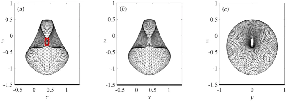
In FIG. 6 (a), two cut lines are found with K = 3 and the numbers of the nodes on the two cut lines are the same in this case. The front and side views of the toroidal bubble are presented in FIG. 6 (b) and (c). At this moment, the mesh quality around the impact position is relatively poor, which can be greatly improved by the present numerical techniques.

FIG. 6. Numerical transition from a singly-connected bubble to a toroidal bubble in the case when two cavitation bubbles are arranged above a rigid wall. In the simulation, the parameters used are R01 = R02 = 0.1911,  = 50. The dimensionless parameters are γbb = 0.8,  = 0 and γbw = 1.5. (a) Front view of the bubble shape just before the jet

impact and two cut lines, (b) front view and (c) side view of the bubble shape after the numerical surgery. The black solid line at the bottom of each frame represents the rigid boundary.

18

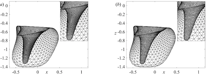
bubble. This interesting physical phenomenon is rarely concerned in previous studies. In order to investigate the subsequent bubble collapse pattern and jetting behaviour, a 3D toroidal bubble splitting model is established here. Firstly, the splitting area is searched by calculating the radius of curvature and limited by a constant ssp, which is defined as the distance between nodes and the axis of symmetry

and set as 0.015Rm for accuracy in the present study. Therefore, the two lines surrounding the splitting area are referred to as the splitting locations, as shown in FIG. 7 (a). Next, the nodes and elements in the splitting area and the nodes on the two splitting locations need to be deleted. Meanwhile, two new nodes are added at two splitting locations, respectively, and new elements are added accordingly. At last, nodes are renumbered and the node information in the elements is updated. Side and 3D views of the bubble profiles after splitting using the newly developed technique are presented in FIG. 7. The subsequent motion after the splitting is well captured and the stability is maintained by using the above numerical techniques.

FIG. 7. Numerical treatment for the splitting of the toroidal bubble for the same case in FIG. 6. (a) Side view of the toroidal bubble at the splitting moment, (b) side view and (c) 3D view of the bubble just after the splitting.

3.Self-coalescence due to self-film-thinning process

One of the highlights in this study is to deal with an extreme situation in which one bubble is attached to the rigid wall at the initial moment. In such kind of ‘contact cases’, the problem can be transformed to the coalescence of three cavitation bubbles. Thus the mirror bubbles are modelled explicitly, and the half-space Green function in Equation (1) is replaced by the simple Green function

1

19

black solid line represents the rigid wall and the evolution of the real bubbles is presented in the upper half part of the figure. In the simulation, the coalescence occurs at two different locations of the three-bubble system, which should be handled simultaneously using the above basic coalescence procedure, as shown in FIG. 8 (a-b). Thereafter, the coalesced bubble continues to expand and the liquid film between the surfaces of the original bubble 1 and its image becomes thinner and thinner, which is called self-film-thinning process in the present study, as shown in FIG. 8 (b). In some ‘contact cases’ (when the angle parameter β is relatively small), the rupture of the thin film may occur, leading to a secondary self-coalescence of the coalesced bubble. As shown in FIG. 8 (c), the minimum distance between the interfaces satisfies the coalescence criterion in the numerical simulation and a self-coalescence technique is applied to handle this partial self-coalescence. At the self-self-coalescence moment, the processing steps are similar to those in the basic coalescence procedure. At first, all the nodes on the coalescence surfaces must satisfy

1 .

i bw c

z   b s (35)

20

FIG. 8. Bubble profiles (a) at the moment of the coalescence of three bubbles, (b) in the self-film-thinning process, (c) just prior to the self-coalescence moment and (d) just after self-coalescence procedure. In the simulation, the parameters used are R0 = 0.1911,  = 50. The angle between the line connecting two inception centres and the rigid wall is β = 0.73. The dimensionless distances are γbw1 = 0.4 and bb = 0.6.

IV.

MODEL VALIDATION AND APPLICATIONS

A. Convergence study

In this section, the effect of the mesh resolution on the 3D simulation results is first investigated. Coalescence of two cavitation bubbles above a rigid wall in an axisymmetric configuration is simulated using the present 3D model and a verified axisymmetric model 23_{. The node numbers (N}

n) on the 3D

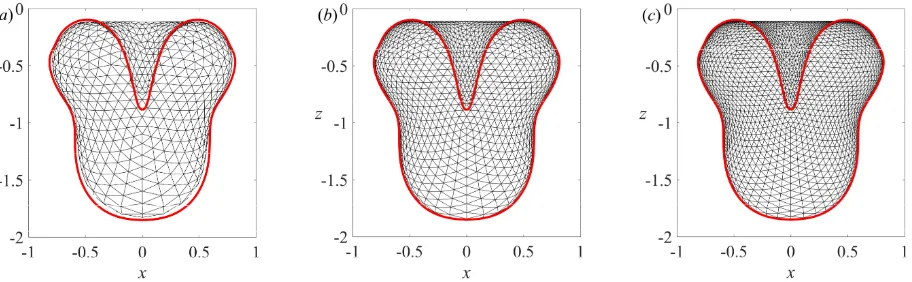
bubble surface are set as 642, 1442 and 2562, respectively. The 3D results are overlaid with the result obtained by axisymmetric model (denoted by the solid red lines), as shown in FIG. 9. The dimensionless parameters are set as: γbb = 0.8, γbw2 = 1.2,  = 50, R01 = R02 =0.1911. The coalesced bubble is seen elongating in the vertical direction and a downward jet forms in the collapse phase. As the node number increases, the 3D results approach to the axisymmetric results, including the overall shape and the sharp jet formation, which indicates the convergence of the numerical model. In the following simulation, Nn = 2562 is selected to ensure the accuracy. In this case, the CPU time to

21

FIG. 9. The jet formation at t_* = 2.634 for an axisymmetric case with γbb = 0.8 and γbw2 = 1.2 with various node numbers: (a) Nn = 642, (b) Nn = 1442 and (c) Nn = 2562 compared with the axisymmetric model (red solid line).

B. Comparison between experiments and 3D simulations

To further validate the present 3D model, comparisons are carried out between experiments and the 3D numerical simulations. In the present study, an underwater electric discharge method is used to generate cavitation bubbles and similarly sized bubbles are generated simultaneously by using a series connection. Details about the experimental setup refer to the work by Han et al 23_{. The relationship}

between the maximum bubble radius and the discharge voltage can be found in Li et al 56_{. When the}

discharge voltage is less than 500V, the uncertainty of the maximum bubble radius in dimensionless form is within 2%. In the present study, the discharge voltage is taken as 500 V. In the experiments, two cavitation bubbles are arranged in an oblique line and the size difference between them is within 20 %. The transient process of two-bubble interaction and coalescence in the non-contact and contact cases are captured by a Phantom V711 high-speed camera working at 60 000 frames/s and 25 000 frames/s, respectively, both with an exposure time of 10 μs. The spatial resolution of the experimental images is around 0.17 mm per pixel.

1.Non-contact case

In the first experiment, the maximum equivalent radii of bubble 1 and bubble 2 are 13.1 mm and 11.1 mm, respectively. The method to determine the maximum equivalent radius of a non-spherical bubble can be found in Li et al 56_{. Other parameters in the experiment are: d}

22

23 (a)

(b)

FIG. 10. Comparison of (a) the experiment with (b) the 3D BIM computation for bubble behaviours at selected times for the coalescence of two cavitation bubbles near a rigid wall. In the experiment, the parameters are Rmax1 = 13.1 mm, Rmax2 = 11.1 mm, dbw1 = 18.75 mm, dbw2 = 10.8 mm and dbb = 8.33 mm. The angle between the axis

connecting inception centres and the rigid wall is β = 1.27. In the simulation, dimensionless parameters used are γbw1 = 1.43, γbw2 = 0.82, γbb = 0.64,  = 50, R01 = 0.1911, R02 = 0.1625. The time is placed at the top of each frame (Multimedia view).

24

the top and the bottom of the two bubbles or the coalesced bubble) and the locations of the two poles are presented in FIG. 11. In general, an overall agreement is achieved except for some small differences, demonstrating the validity of the present model.

FIG. 11. Quantitative comparisons between the numerical simulation and the experiment.Time evolutions of (a) the bubble heighthb and (b) the locations of the north and south poles of the bubbles.

2.Contact case

In the second experiment, the initial centre of cavitation bubble 2 is placed on the rigid wall, i.e. an attached case. The maximum equivalent radii of bubble 1 and bubble 2 are 12.5 mm and 13.4 mm, respectively. Other parameters in the experiment are: dbb = 12.9 mm and β = 0.79. The dynamic

behaviours of cavitation bubbles are captured by the high-speed camera with the time interval being 40 μs between two frames. In the computation, dimensionless parameters used are γbw1 = 0.79, γbb =

25

bubbles occurs in the expansion phase (frames 2-3). In the collapse phase, the bubble bottom remains attached to the boundary with a slow contraction in width, while the bubble surface far away from the rigid wall collapses fast and forms an oblique liquid jet (frames 4-6). The essential physical features of such extreme case is extremely well reproduced by the present 3D simulation, as shown in FIG. 12 (b), demonstrating the robustness and high-accuracy of the present model.

It is well known that the violent jet impact is one of the main cause of cavitation erosion 24, 39, 57_.

In this case, the jet impacts directly on the rigid wall and a toroidal bubble is formed in the simulation. The subsequent motion of the toroidal bubble is also simulated and the upper half of the toroidal bubble shape is presented in FIG. 13, together with the velocity and pressure fields in the flow to reveal more

(a)

(b)

26

physical mechanisms. A high-pressure region of which the pressure peak decreases gradually with time (marked with A in frame a), as the direct driving force of the jet formation, can be observed at the base of the oblique jet at these two moments. A more pronounced localised high-pressure region is generated by the direct jet impact on the rigid wall (frame a). This high-pressure region and the continuous inflow of the liquid from the jet leads to the formation of a horizontal jet directed leftward. Meanwhile, the left surface of the toroidal bubble continues collapsing along the rigid wall and finally collides with the horizontal jet (frame b). It is noted that the liquid jet persistently impacts the rigid wall and the inner gas pressure increases during the shrink of the bubble volume, resulting in a rapid increase of the hydrodynamic force on the wall.

FIG. 13. Toroidal bubble evolution with the velocity and pressure fields in the flow for the same case in FIG. 12. The dimensionless times are t_* = (a) 2.642 and (b) 2.680 (the time scale is 1.258 ms).

C. Model applications

1.Self-coalescence of a coalesced bubble

27

The surface of bubble 1 is flattened by bubble 2 and the lower rigid wall simultaneously due to its close proximity to the rigid boundary (frames a and b). During the subsequent expansion of the coalesced bubble, the bottom of the original bubble 1 and the top of its image become very close (frame c). As one of the highlights in the numerical development, a self-coalescence technique described in Section III C is proposed to handle such process in this study. After self-coalescence disposal, the bubble keeps expanding and the maximum volume is reached in frame (d). In the collapse phase, the left surface and the upper right surface of the coalesced bubble collapse earlier and faster (frame e), and a horizontal jet and an oblique jet form afterwards, respectively (frame f). Such kind of phenomenon is often observed when both bubbles are very close to the rigid wall and β is less than ~π/4. The self-coalescence technique has been demonstrated to work quite well and robust when dealing with this problem.

FIG. 14. Bubble profiles with the total velocity contours on bubble surface. The dimensionless times in the computation are t* = (a) 0.043, (b) 0.459, (c) 0.736, (d) 0.957, (e) 2.044 and (f) 2.776. In the simulation, the

parameters used are R0 = 0.1911,  = 50. The angle between the line connecting two inception centres and the rigid wall is β = 0.73. The dimensionless distances are γbw1 = 0.4 and bb = 0.6. The dimensionless times in the

28

2.Toroidal bubble splitting

In this section, the bubble coalescence characteristics at different phases for another interesting case will be examined when two bubbles are in a horizontal configuration. The dimensionless parameters in the simulation are bw = 1.5, bb = 0.8, = 50 and R0 = 0.1911. The bubble evolution before the jet impact is given in FIG. 15, together with the velocity contours on the bubble surface. The bubbles coalesce in the expansion phase and the circular edges of the coalescence surfaces exhibits the largest velocity (frame 1), resulting in the annular swelling of the coalesced bubble (frame 2). The bubble bottom is still expanding at the moment of maximum volume moment with higher velocity than other parts (frame 2). In the collapse phase, two oblique jets are formed due to the co-effect of the other bubble and the rigid wall (frames 3-4) and finally about to collide at t_* = 2.642 (frame 5). An

obvious downward migration of the two bubbles is observed due to the attraction of the rigid wall. It is worth noting that the existence of a second bubble alters the jet direction of the first bubble. Therefore, the jet impact threat to a nearby rigid wall may be decreased by the interaction of multiple bubbles. The flow field pressure and the subsequent toroidal bubble dynamics will be further investigated as follows.

FIG. 15.Bubble profiles before jet impact with the total velocity contours on bubble surface. In the simulation, the dimensionless parameters used are bw = 1.5, bb = 0.8,  = 50 and R0 = 0.1911. The dimensionless times are marked at the top of each frame.

29

fields surrounding the coalesced bubble are calculated; while in 3D view, the pressure on the rigid wall is given. In FIG. 16 (a), two high-pressure regions are observed in the front view, which promotes the development of the two oblique jets. It is noted that the pressure above the bubble is higher than that between the bubble and the rigid wall, leading to a faster collapse of the bubble top and the migration of the bubble towards the wall. As the bubble top contracts, a localised high-pressure region is gradually formed above the bubble and can be observed in frame (b). The formation of the high-pressure region is similar to that in single-bubble-wall interaction, which may cause the formation of a jet directed towards the wall.

After the jet impact (frame c), the collision of the two oblique jets leads to the high-pressure region inside the bubble, which is much higher than that surrounding the outer profile of the bubble surface. The high pressure around the bubble top drives the part of the toroidal bubble further away from the wall to collapse very fast. The continuous impact of the liquid around the bubble top finally leads to a very high peak pressure at the splitting moment, as shown in (d). The high-pressure amplitude at the splitting location increases rapidly due to the focusing flow. The two ends of the bubble contract very fast afterwards and the pressure region gradually separates into two high-pressure regions (frames e and f), which promote the formations of two jets at the two ends. Finally, the two thin jets penetrate the side wall of the bubble (frame g). From the 3D views in FIG. 16 (a)-(f), it is noted that the pressure on the rigid wall is nearly symmetrically distributed under all rotations about the centre and increases outwards; while at the jet impact moment (frame g), a different pressure distribution can be observed, i.e. an annular high-pressure region is formed on the wall. It is worth noting that the subsequent stage of the bubble motion is beyond the capacity of the BIM. Nevertheless, we can predict that the bubble will migrate towards the wall but the focusing energy of the bubble may be weakened by the multiple jets.

30 (b)

(c)

(d)

31 (f)

(g)

FIG. 16. Bubble evolution with the pressure fields in the flow for the same case in FIG. 15. The dimensionless times are t_* = (a) 2.496, (b) 2.642, (c) 2.687, (d) 2.706, (e) 2.707, (f) 2.723 and (g) 2.773, respectively. Both the front view, side view and 3D view of bubble shape at each moment are presented. In the simulation, the dimensionless parameters of two cavitation bubbles are R0 = 0.1911,  = 50, γbb = 0.8, γbw = 1.5 and β = 0.

3.Two cavitation bubbles attached to the rigid wall

32

coalescence criterion between the real bubble and the image bubble is satisfied at t_* = 1.315 (frame c).

At this moment, the present problem is transformed to the coalescence of the coalesced bubble and its image across the boundary so that the subsequent motion can be numerically simulated. In frame (d), the maximum volume is attained and the bubble surface on the rigid wall exhibits the highest velocity and is still expanding. In the collapse phase, the contractions of the upper left and upper right parts of the coalesced bubble occur earlier and two oblique jets are gradually developed, while the top of the bubble collapses slowly (frames e-g). At the late collapse stage, the total velocity of the bubble top continues to increase due to the Bjerknes force from the rigid wall and there is a tendency to form a downward jet (frame h). In frame (i), the bubble shape in top view is presented on the top right corner and the dent at the bubble top clearly exhibits the highest velocity, which is squeezed by the two oblique jets in the collapse phase. Before the jet impact on the wall, these two jets will collide inside the bubble, which is believed to decrease the damage potential of jet impact.

FIG. 17. Bubble profiles before jet impact with the total velocity contours on bubble surface. The corresponding

times are t* = (a) 0.162, (b) 0.837, (c) 1.315, (d) 1.543, (e) 1.930, (f) 2.423, (g) 2.748, (h) 2.858 and (i) 2.909,

33

The dimensionless times in the computation and the frame number are marked at the corner of each frame.

FIG. 18. The pressure and velocity fields surrounding a coalesced bubble sitting on a rigid wall. The dimensionless times are t_* = (a) 2.423, (b) 2.748, (c) 2.858 and (d) 2.909, corresponding to frames (f)-(i) in FIG. 17.

To further demonstrate capability and robustness of the present numerical model, computational results capable of revealing the detailed dynamics of the bubble coalescences near a rigid wall during different phases including the velocity and pressure fields in the flow at four typical moments are given in FIG. 18, corresponding to frames (f)-(i) in FIG. 17. The fast contraction of the bubble draws the surrounding liquid and a high-pressure region is formed around the top of the bubble (frame b), which promotes the shrink of the bubble top and may also lead to the formation of a downward jet. As the collapse continues, the high-pressure region becomes more localised with a higher pressure peak. It is observed that the surrounding liquid is drawn into the three jets and the two oblique jets keep squeezing the downward jet, which may result in partial splitting of the bubble.

V.

CONCLUSIONS AND OUTLOOK

34

concerned previously. All cases studied in this paper are of paramount importance to practical engineering applications. In the present model, there is no lower limit of the stand-off distance between bubbles and the nearby rigid wall,which is crucial to predicting and understanding the attached bubble behaviours in cavitation and many other applications. A density potential method (DPM) combined with a simple but effective remesh scheme is used to achieve a desired high-quality mesh distribution. Meanwhile, a weighted moving least-square smoother is encapsulated in the code to eliminate numerical instabilities. Advanced topological techniques are developed to handle complex dynamic behaviours involved in the multi-bubble coalescence. The validation of the 3D model is confirmed by comparisons with the axisymmetric model and two experiments. The highly non-spherical bubble behaviours are well reproduced by the simulations, including the surface flattening of two approaching bubbles, multi-jet formation of a coalesced bubble, splitting of a toroidal bubble and a self-coalescence due to the self-film-thinning process, indicating the stability and robustness of the present 3D model. A number of new physical phenomena are found from the numerical computations in the present study. Nevertheless, a systematic study of the governing parameters will be for our future work.

Besides, the present universal topological treatment is suitable for complex topology changes involved in coalescence problems and the implementation of the advanced numerical schemes are beneficial to improving mesh quality. As an outlook, the present model can also be adopted to study droplet dynamics58-60_{if some factors including surface tension are carefully considered.}

ACKNOWLEDGEMENTS

This work is supported by the National Natural Science Foundation of China (11702071 and 51709056), the National Key R&D Program of China (2018YFC0308900), the China Postdoctoral Science Foundation (2017M620112, 2018T110276 and 2017M621249) and the Heilongjiang Postdoctoral Fund (LBH-Z17049).

REFERENCES

1. J. R. Blake, and D. Gibson, "Cavitation bubbles near boundaries," Annual Review of Fluid Mechanics 19, 99 (1987).

2. C. E. Brennen, "Cavitation and Bubble Dynamics," (1995).

35

361, 75 (1998).

4. E.-A. Brujan, T. Noda, A. Ishigami, T. Ogasawara, and H. Takahira, "Dynamics of laser-induced cavitation bubbles near two perpendicular rigid walls," Journal of Fluid Mechanics 841, 28 (2018).

5. A. M. Zhang, S. Li, and J. Cui, "Study on splitting of a toroidal bubble near a rigid boundary," Physics of Fluids

27, 809 (2015).

6. P. Cui, A.-M. Zhang, S. Wang, and B. C. Khoo, "Ice breaking by a collapsing bubble," Journal of Fluid Mechanics

841, 287 (2018).

7. Y. Zhang, Y. Zhang, Z. Qian, B. Ji, and Y. Wu, "A review of microscopic interactions between cavitation bubbles and particles in silt-laden flow," Renewable and Sustainable Energy Reviews 56, 303 (2016).

8. J. Blake, P. Robinson, A. Shima, and Y. Tomita, "Interaction of two cavitation bubbles with a rigid boundary," Journal of Fluid Mechanics 255, 707 (1993).

9. P. B. Robinson, J. R. Blake, T. Kodama, A. Shima, and Y. Tomita, "Interaction of cavitation bubbles with a free surface," Journal of Applied Physics 89, 8225 (2001).

10. N. Saleki-Haselghoubi, M. T. Shervani-Tabar, M. Taeibi-Rahni, and A. Dadvand, "Interaction of two spark-generated bubbles near a confined free surface," Theoretical and Computational Fluid Dynamics 30, 185 (2016). 11. Y. Zhang, Y. Zhang, and S. Li, "The secondary Bjerknes force between two gas bubbles under dual-frequency acoustic excitation," Ultrasonics Sonochemistry 29, 129 (2016).

12. G. L. Chahine, and C.-T. Hsiao, "Modelling cavitation erosion using fluid–material interaction simulations," Interface focus 5, 20150016 (2015).

13. G. L. Chahine, A. Kapahi, J. K. Choi, and C. T. Hsiao, "Modeling of surface cleaning by cavitation bubble dynamics and collapse," Ultrasonics Sonochemistry 29, 528 (2016).

14. F. Reuter, and R. Mettin, "Mechanisms of single bubble cleaning," Ultrasonics sonochemistry 29, 550 (2016). 15. E. Cox, A. Pearson, J. R. Blake, and S. R. Otto, "Comparison of methods for modelling the behaviour of bubbles produced by marine seismic airguns," Geophysical prospecting 52, 451 (2004).

16. C. T. Hsiao, J. Choi, S. Singh, G. L. Chahine, T. A. Hay, Y. A. Ilinskii, E. A. Zabolotskaya, M. F. Hamilton, G. Sankin, F. Yuan, and P. Zhong, "Modelling single- and tandem-bubble dynamics between two parallel plates for biomedical applications," Journal of Fluid Mechanics 716, 137 (2013).

17. S. W. Fong, D. Adhikari, E. Klaseboer, and B. C. Khoo, "Interactions of multiple spark-generated bubbles with phase differences," Experiments in Fluids 46, 705 (2009).

18. L. W. Chew, E. Klaseboer, S.-W. Ohl, and B. C. Khoo, "Interaction of two differently sized oscillating bubbles in a free field," Physical Review E 84, 066307 (2011).

19. L. W. Chew, E. Klaseboer, S.-W. Ohl, and B. C. Khoo, "Interaction of two oscillating bubbles near a rigid boundary," Experimental Thermal and Fluid Science 44, 108 (2013).

20. N. Bremond, M. Arora, S. M. Dammer, and D. Lohse, "Interaction of cavitation bubbles on a wall," Physics of Fluids 18, 121505 (2006).

21. S. Rungsiyaphornrat, E. Klaseboer, B. Khoo, and K. Yeo, "The merging of two gaseous bubbles with an application to underwater explosions," Computers & Fluids 32, 1049 (2003).

22. R. Han, S. Li, A. M. Zhang, and Q. X. Wang, "Modelling for three dimensional coalescence of two bubbles," Physics of Fluids 28, 062104 (2016).

23. R. Han, A. M. Zhang, S. Li, and Z. Zong, "Experimental and numerical study of the effects of a wall on the coalescence and collapse of bubble pairs," Physics of Fluids 30, 042107 (2018).

24. S. Li, R. Han, A. Zhang, and Q. Wang, "Analysis of pressure field generated by a collapsing bubble," Ocean Engineering 117, 22 (2016).

36

an application to cavitation in silt-laden flow," Physics of Fluids 30, 082111 (2018).

26. S. P. Wang, A. M. Zhang, Y. L. Liu, S. Zhang, and P. Cui, "Bubble dynamics and its applications," Journal of Hydrodynamics 30, 975 (2018).

27. G. Falcucci, E. Jannelli, S. Ubertini, and S. Succi, "Direct numerical evidence of stress-induced cavitation," Journal of Fluid Mechanics 728, 362 (2013).

28. G. L. Chahine, and T. O. Perdue, Simulation of the three‐dimensional behavior of an unsteady large bubble near a structure (AIP Publishing, 1990).

29. G. L. Chahine, K. M. Kalumuck, and C. T. Hsiao, "Simulation of surface piercing body coupled response to underwater bubble dynamics utilizing 3DYNAFS, a three-dimensional BEM code," Computational Mechanics 32, 319 (2003).

30. Y. L. Zhang, K. S. Yeo, B. C. Khoo, and C. Wang, "3D Jet Impact and Toroidal Bubbles," Journal of Computational Physics 166, 336 (2001).

31. C. Wang, and B. C. Khoo, "An indirect boundary element method for three-dimensional explosion bubbles," Journal of Computational Physics 194, 451 (2004).

32. B. H. T. Goh, S. W. Gong, S.-W. Ohl, and B. C. Khoo, "Spark-generated bubble near an elastic sphere," International Journal of Multiphase Flow 90, 156 (2017).

33. S. W. Gong, S. W. Ohl, E. Klaseboer, and B. C. Khoo, "Interaction of a spark-generated bubble with a two-layered composite beam," Journal of Fluids and Structures 76, 336 (2018).

34. Z. Zong, J. X. Wang, L. Zhou, and G. Y. Zhang, "Fully nonlinear 3D interaction of bubble dynamics and a submerged or floating structure," Applied Ocean Research 53, 236 (2015).

35. S. Li, A. M. Zhang, R. Han, and Q. Ma, "3D full coupling model for strong interaction between a pulsating bubble and a movable sphere," Journal of Computational Physics (2019).

36. E. Klaseboer, B. C. Khoo, and K. C. Hung, "Dynamics of an oscillating bubble near a floating structure," Journal of Fluids and Structures 21, 395 (2005).

37. B. M. Borkent, M. Arora, C. D. Ohl, N. De Jong, M. Versluis, D. Lohse, K. A. MØrch, E. Klaseboer, and B. C. Khoo, "The acceleration of solid particles subjected to cavitation nucleation," Journal of Fluid Mechanics 610, 157 (2008).

38. A. Zhang, and Y. Liu, "Improved three-dimensional bubble dynamics model based on boundary element method," Journal of Computational Physics 294, 208 (2015).

39. R. Tong, W. Schiffers, S. Shaw, J. Blake, and D. Emmony, "The role of'splashing'in the collapse of a laser-generated cavity near a rigid boundary," Journal of Fluid Mechanics 380, 339 (1999).

40. E. A. Brujan, G. S. Keen, A. Vogel, and J. R. Blake, "The final stage of the collapse of a cavitation bubble close to a rigid boundary," Physics of Fluids 14, 85 (2002).

41. Y. Tomita, P. Robinson, R. Tong, and J. Blake, "Growth and collapse of cavitation bubbles near a curved rigid boundary," Journal of Fluid Mechanics 466, 259 (2002).

42. S. R. Gonzalez-Avila, E. Klaseboer, B. C. Khoo, and C.-D. Ohl, "Cavitation bubble dynamics in a liquid gap of variable height," Journal of Fluid Mechanics 682, 241 (2011).

43. O. Supponen, D. Obreschkow, M. Tinguely, P. Kobel, N. Dorsaz, and M. Farhat, "Scaling laws for jets of single cavitation bubbles," Journal of Fluid Mechanics 802, 263 (2016).

44. J. Best, "The formation of toroidal bubbles upon the collapse of transient cavities," Journal of Fluid Mechanics

251, 79 (1993).

45. L. Rayleigh, "VIII. On the pressure developed in a liquid during the collapse of a spherical cavity," The London, Edinburgh, and Dublin Philosophical Magazine and Journal of Science 34, 94 (1917).

37

and numerical investigation of the dynamics of an underwater explosion bubble near a resilient/rigid structure," Journal of Fluid Mechanics 537, 387 (2005).

47. R. Han, A. m. Zhang, and S. Li, "Three-dimensional numerical simulation of crown spike due to coupling effect between bubbles and free surface," Chinese Physics B 23, 034703 (2014).

48. Q. Wang, "The evolution of a gas bubble near an inclined wall," Theoretical and Computational Fluid Dynamics

12, 29 (1998).

49. C. Wang, B. C. Khoo, and K. S. Yeo, "Elastic mesh technique for 3D BIM simulation with an application to underwater explosion bubble dynamics," Computers & Fluids 32, 1195 (2003).

50. Q. X. Wang, "Numerical simulation of violent bubble motion," Physics of Fluids 16, 1610 (2004).

51. Q. X. Wang, and K. Manmi, "Three dimensional microbubble dynamics near a wall subject to high intensity ultrasound," Physics of Fluids 26, 032104 (2014).

52. R. E. Bank, and J. Xu, "An algorithm for coarsening unstructured meshes," Numerische Mathematik 73, 1 (1996). 53. D. A. Field, "Qualitative measures for initial meshes," International Journal for Numerical Methods in Engineering 47, 887 (2000).

54. Q. X. Wang, "Unstructured MEL modelling of nonlinear unsteady ship waves," Journal of Computational Physics

210, 368 (2005).

55. Q. Wang, K. Manmi, and M. L. Calvisi, "Numerical modeling of the 3D dynamics of ultrasound contrast agent microbubbles using the boundary integral method," Physics of Fluids 27, 022104 (2015).

56. S. Li, B. C. Khoo, A. M. Zhang, and S. Wang, "Bubble-sphere interaction beneath a free surface," Ocean Engineering 169, 469 (2018).

57. C. T. Hsiao, A. Jayaprakash, A. Kapahi, J. K. Choi, and G. L. Chahine, "Modelling of material pitting from cavitation bubble collapse," Journal of Fluid Mechanics 755, 142 (2014).

58. A. Montessori, P. Prestininzi, M. La Rocca, and S. Succi, "Entropic lattice pseudo-potentials for multiphase flow simulations at high Weber and Reynolds numbers," Physics of Fluids 29, 092103 (2017).

59. W. Bouwhuis, R. C. van der Veen, T. Tran, D. L. Keij, K. G. Winkels, I. R. Peters, D. van der Meer, C. Sun, J. H. Snoeijer, and D. Lohse, "Maximal air bubble entrainment at liquid-drop impact," Physical Review Letters 109, 264501 (2012).