Perceptions of randomness in binary sequences: Normative, heuristic, or both?

City, University of London Institutional Repository

Citation

:

10.1016/j.cognition.2017.11.002

This is the accepted version of the paper.

This version of the publication may differ from the final published

version.

Permanent repository link:

Link to published version

:

Copyright and reuse:

City Research Online aims to make research

outputs of City, University of London available to a wider audience.

Copyright and Moral Rights remain with the author(s) and/or copyright

holders. URLs from City Research Online may be freely distributed and

linked to.

City Research Online: http://openaccess.city.ac.uk/ [email protected]

Perceptions of randomness in binary sequences: Normative, heuristic, or both?

Stian Reimers 1, 2

Chris Donkin 3

Mike E. Le Pelley 3, 4

1

City, University of London, UK

2

University College London, London, UK.

3

University of New South Wales, Sydney, Australia

4

Cardiff University, Cardiff, UK

Please address correspondence to:

Dr Stian Reimers

Department of Psychology

City, University of London

Northampton Square

London EC1V 0HB

United Kingdom

Abstract

When people consider a series of random binary events, such as tossing an unbiased coin and

recording the sequence of heads (H) and tails (T), they tend to erroneously rate sequences with

less internal structure or order (such as HTTHT) as more probable than sequences containing

more structure or order (such as HHHHH). This is traditionally explained as a local

representativeness effect: Participants assume that the properties of long sequences of random

outcomes—such as an equal proportion of heads and tails, and little internal structure—should

also apply to short sequences. However, recent theoretical work has noted that the probability of

a particular sequence of say, heads and tails of length n, occurring within a larger (>n) sequence

of coin flips actually differs by sequence, so P(HHHHH) < P(HTTHT). In this alternative

account, people apply rational norms based on limited experience. We test these accounts.

Participants in Experiment 1 rated the likelihood of occurrence for all possible strings of 4, 5, and

6 observations in a sequence of coin flips. Judgments were better explained by representativeness

in alternation rate, relative proportion of heads and tails, and sequence complexity, than by

objective probabilities. Experiments 2 and 3 gave similar results using incentivized binary choice

procedures. Overall the evidence suggests that participants are not sensitive to variation in

objective probabilities of a sub-sequence occurring; they appear to use heuristics based on several

distinct forms of representativeness.

1. Introduction

Many of the judgments that humans make are based on the abstraction of patterns in events

that occur in the world. These patterns can take many forms, such as weather – deciding whether

to take a coat or an umbrella based on the temperature and rainfall of previous days – the

behaviour of other individuals – guessing when a co-author is likely to complete a manuscript

draft based on their previous timeliness – or the behavior of wider groups of people – forecasting

sales for upcoming months based on figures from recent months.

One of the challenges of any pattern-detection system, whether human or artificial, is to separate

signal from noise: to extract, and base predictions on, systematic patterns that appear in the

environment, and ignore observations that are—to the system at least—random. If distinguishing

between regularity (which has predictive value) and randomness (which does not) is a basic

requirement for making successful predictions about the environment, it is surprising that, in

higher-level cognition at least, humans are relatively poor at recognizing randomness (for reviews

see, Nickerson, 2002, 2004; Bar-Hillel & Wagenaar, 1991; Falk & Konold, 1997; for a similar

overview of randomness production, see Rapaport & Budescu, 1997).

Most empirical research examining human (mis-) understanding of randomness has used

equiprobable binary outcomes (see Oskarsson, Van Boven, McClelland, & Hastie, 2009, for a

review), such as the occurrence of red or black on a roulette wheel (e.g., Ayton & Fischer, 2004),

or birth order of boys and girls in a particular family (Kahneman & Tversky, 1972). The most

common scenario is the occurrence of heads and tails when repeatedly tossing a fair, unbiased

coin (e.g., Caruso, Waytz & Epley, 2010; Kareev, 1992; Diener & Thompson, 1985). Across a

variety of tasks—including choosing the most random of a set of sequences (e.g. Wagenaar,

1970), classifying individual sequences as random or non-random (e.g., Lopes & Oden, 1987),

and prediction of future outcomes of a sequence of coin tosses or roulette wheel spins (e.g.,

generating mechanism.

The mischaracterizations that people make are similar across different types of task. They

include (using Hahn & Warren’s, 2009, characterization): (a) a preference for negative recency

between trials rather than independence, meaning that in binary outcomes there is an expectation

of an alternation rate between outcomes of greater than .5.; (b) a belief that in short sequences,

equiprobable outcomes should occur equally often; and (c) a belief that an unstructured or

unordered appearance indicates that a sequence of outcomes is more random and hence more

likely to occur from a random process (see, e.g., Wagenaar, 1970; Falk & Konold, 1997). These

biases lead to participants showing a gambler’s fallacy for random events (e.g., Ayton & Fischer,

2004), or a hot-hand bias for events under human control (Gilovich, Valone, & Tversky, 1995;

but see Miller & Sanjurjo, 2014, 2016): Following a run of the same outcome from a random

process, such as five heads in a row in a coin tossing procedure, participants rate the probability

of the same outcome occurring again as lower than following other sequences for sequences

believed to be generated randomly (gambler’s fallacy, showing negative recency), and rate the

probability as higher for sequences that could be under human control (hot-hand, positive

recency). Similar effects are seen using continuous outcome measures in forecasting: participants

make forecasts that reflect an assumption of serial dependence in a time series, when outcomes

are in fact random (Reimers & Harvey, 2011).

In one of the most influential studies in randomness perception, Kahneman and Tversky

(1972) conducted two experiments in which participants estimated the relative frequency of two

birth orders of boys (B) and girls (G) across families with six children in a city: GBGBBG or

BGBBBB. Participants judged that there would be far fewer families with BGBBBB than

GBGBBG, suggesting a more representative 1:1 ratio of boys and girls was more likely. However

participants also rated BBBGGG as less likely to occur than GBGBBG, suggesting the structure

representativeness (which we discuss below), has been the dominant explanation for human

judgments of random sequences.

In this paper, we examine some of the ways in which people mischaracterize randomness.

Specifically, explanations for deviations from normativity in randomness tasks have traditionally

taken a heuristics and biases approach (Kahneman & Tversky, 1972). More recent theoretical

approaches have emphasized the potential for apparent biases to reflect rational judgments in

situations with limited experience. We discuss these two approaches now.

1.1. Heuristics and biases account

The set of arguments that comes from the heuristics and biases literature suggests

performance can be characterized as the application of a representativeness heuristic to short

sequences of outcomes. We would expect a random binary sequence of infinite length to a have a

number of properties: It should contain the same proportion of each outcome; it should have an

alternation rate of around .5; it should not contain any internal structure that allows it to be

compressed (these properties are discussed further below). The heuristic account argues that

people assume that these properties of infinite-length random sequences will also tend to be

expected to be seen in short, exact strings of random outcomes. If they are not, a string is judged

to be less random or less likely to be generated by a random process. But in reality they are not:

for example, in a series of four coin tosses, the chance of tossing four heads in a row (HHHH),

and HTTH is equal, at one-sixteenth. By misapplying a representativeness heuristic to short,

exact strings of outcomes, participants would rate unrepresentative-looking outcomes (such as

HHHH) as being less likely to occur through a random process than are more

representative-looking outcomes (e.g., HTTH).

The notion of representativeness has, however, been criticized as nebulous and untestable.

specification, and therefore offer enough flexibility to risk being unfalsifiable, and can between

them be used to make a post hoc account of almost any experimental finding. Ayton and Fischer

(2004) noted that representativeness was used to account for both the gambler’s fallacy, and its

opposite, the hot-hand fallacy. Falk and Konold (1997) also noted that there was no a priori way

of predicting how representativeness might affect performance on a task, making falsifiable

predictions difficult.

Kahneman and Tversky (1972) did make some attempt to define representativeness in

binary randomness tasks. As noted above, they suggested that the relative proportions of the two

outcomes might be important. In addition, strings containing more alternations (e.g., HHTHTH,

which contains four alternations) typically appear more representative of a random generation

process than strings containing fewer alternations (e.g., HHHHTT, which contains one

alternation). Strings with relatively few alternations tend to contain long runs of a single outcome

type, which are heuristically unrepresentative of a random generation process. (Of course, these

attributes are not independent: High alternation rates tend to have shorter runs, and vice versa.

See Scholl & Greifeneder, 2011, for an attempt to disambiguate the role of run length and

alternation rate in longer sequences of outcomes.)

Finally, a random generation process should produce sequences that are uncompressible;

that is, that contain no internal structure that allows them to be expressed any more concisely than

by giving the entire sequence. For example, HHHHHHHHHHHH could be compressed as (H ×

12), or HHTHHTHHTHHT could be compressed as (HHT × 4). In contrast, HTHHTTTHTHHT

is not so easily compressed. On this basis, Kahneman and Tversky noted that strings of outcomes

that can be given descriptive short-cuts (e.g., HTHTHT being “HT three times”) appear less

random. This was more formally codified in Falk and Konold’s (1997) Difficulty Predictor (DP).

Although DP primarily attempted to capture the subjective difficulty of encoding a sequence of

also Gauvrit Singmann, Soler-Toscano, & Zenil, 2015, for a method of calculating

Kolmogorov-Chaitin complexity for short binary strings. For longer sequences, formal and subjective

compressibility may diverge due to cognitive limitations.). As complexity is one way of defining

the randomness of a sequence, use of DP in judgments could be seen as reflecting the

misapplication of a norm in which participants make their judgments based on the entropy of a

sequence, rather than its probability of occurrence.

The idea that several different properties may contribute to the representativeness of a

string introduces further degrees of freedom to the heuristic-based account, and renders it

correspondingly difficult to test. In particular, the relative influence, under an account of local

representativeness, of proportions, alternations, and compressibility, is something that remains

untested. Examining the extent to which one kind of representativeness is more important than

others in guiding randomness performance could help with understanding the representations and

processes involved, and constrain local representativeness predictions for other situations. This is

one of the aims of the current experiments.

1.2. Experiential account

An alternative set of arguments treats apparent biases in randomness judgments as adaptive

responses to environmental experience. Several authors have noted that events in the world may

exhibit negative recency, that is, immediately following an outcome, the same outcome is less

likely to occur again. For example, after several days of rain, the nature of weather patterns may

make it less likely that rain will continue the following day (see, e.g., Ayton & Fischer, 2004;

Pinker, 1997).

More abstractly, participants may confuse sampling with replacement and sampling without

replacement (see Fiorina, 1971; Morrison & Ordeshook, 1975, for early discussion of this

containing 10 red and 10 green without replacement, after drawing 4 reds in a row, the

probability of the next bead being green is greatly increased. Many real-world samples involve

drawing without replacement, which may encourage more general assumptions of negative

recency in randomness judgments, either through overgeneralization or through misconstruing

the experimental environment (Hahn & Warren, 2009; Ayton & Fischer, 2004).

There is also a set of models that build on counterintuitive properties of random sequences,

suggesting that erroneous or biased judgments might reflect the (mis-) application of alternative

norms; that is, accurately representing one’s experience of random sequences, but misapplying

that experience when asked to make judgments or choices. For example, Kareev (1992)

demonstrated that participants who were instructed to generate random sequences, tended to

produce typical sequences with respect to the number of heads and tails they contained. This was

accounted for by noting that across all 1024 possible sequences of 10 coin flips, 252 contained

exactly 5 heads, whereas, for example, only 10 contained 9 heads. Thus, the most frequent

number of heads is 5, and sequences containing exactly 5 heads are most typical of 10-item

random sequences. Kareev used this observation to account for overalternation biases seen in

randomness production: If participants generate typical sequences containing 5 heads and 5 tails,

then these sequences will on average have an alternation rate higher than 50%.

As another example, Miller and Sanjuro (2016) recently showed that in a short random

binary sequence of outcomes, the expected proportion of three occurrences of an outcome that

were then followed by the same outcome again was less than .5 (and of course conversely, the

proportion of three outcomes followed by the opposite outcome was greater than .5). Thus,

evidence traditionally seen as supportive of the Hot Hand Fallacy (Gilovich et al., 1985) actually

suggests that it may not be a fallacy.

Most significantly, and of most relevance to this paper, Hahn and Warren (2009) have

specific outcomes are actually less likely to be observed than others (see Reimers, 2017, for a

discussion of similarities between this theory and the work of Miller and Sanjurjo, 2016; see also

Konold, 1995, Nickerson, 2007, and Kareev,1992, for earlier psychologically-motivated work

relating to this phenomenon, and Feller, 1968 for mathematical background). Hahn and Warren’s

argument involved considering strings as component parts of longer sequences of events. While it

is true that the two strings HHTHTT and HHHHTH are equally likely to occur given exactly six

tosses of a coin, it is not the case that these strings are equally likely to occur at least once in any

global sequence of finite length n > 6. The argument is presented in detail by Hahn and Warren

(see also Sun, Tweney & Wang, 2010; Sun and Wang, 2010a , 2010b), and summarized here. For

this purpose, we use the term string to refer to a relatively short sequence of heads and tails that

participants might be asked to make a judgment on, and global sequence to refer to a longer

sequence of heads and tails, generated by tossing a coin, in which that string may appear. For

example, the string THT (with length k = 3) appears three times in the global sequence

HTHTTTTHTHT, which has length n = 11. Note that two of the occurrences overlap.

Figure 1: Raster plot of a sequence of 1,000 simulated coin flips. Vertical lines show where,

between the first flip on the far left and the last flip on the far right, each of the strings occurred.

Note that the total number of occurrences of each string is approximately equal. However,

If the global sequence is infinitely long, then any two strings of the same length k will

occur the same number of times. However, the distribution of these occurrences will not be the

same for all strings: The string HHHH will tend to cluster. Suppose that HHHH appears at

position t in the global sequence (where by ‘appears’ we mean ‘is completed’; i.e. the elements at

positions t – 3, t – 2, t – 1, and t are all H). Consequently, there is a 50% chance that it will

appear again at position t + 1 (i.e., if the coin toss on trial t + 1 yields H, then positions t – 2, t –

1, t, and t + 1 are all H). In contrast, the string HHHT cannot cluster in the same way, because

there is no way for two occurrences of HHHT to overlap – all different occurrences of this string

must be entirely separate. To illustrate this, Figure 1 shows a raster plot of a simulated global

sequence of 1,000 coin flips, with bars marking the points at which each of the strings HHHH

and HHHT occurred. Since the global sequence (n = 1000) is very long relative to the length of

each string (k = 4), the total number of occurrences of HHHH and HHHT in the global sequence

is approximately equal. However, the distribution is very different. Specifically, occurrences of

HHHT are relatively regular (a ‘steady drip’), whereas occurrences of HHHH tend to occur in

irregular clusters, with large gaps in between. This results in significant areas of white space in

the HHHH sequence, where HHHH did not occur for many flips.

The upshot is that there are many more windows of a given sequence length (n > 4) that do

not contain the string HHHH than do not contain the string HHHT: In a sequence of length, say,

20, the probability that the string HHHH does not occur (which we label PGN , standing for

probability in the Global sequence of Non-occurrence, following Sun et al.’s terminology) is

greater (at around .5) than the equivalent probability for HHHT (at around .25). Equivalently, the

probability that HHHH occurs at least once as part of this global sequence of 20 tosses (labeled

PGO, standing for the probability in the Global sequence of Occurrence) is less than for HHHT.

Hahn and Warren noted that people’s experiences of random sequences such as coin tosses

Consequently, in the sequences that people have observed, there is a greater probability of not

observing HHHH than not observing HHHT. When asked by a cognitive psychologist to pick

which of HHHH or HHHT is more likely, if people assume this question refers to occurrence in a

similar finite sample, then their preference for the latter should not be classed as an error; instead

it is a sensible inference based on their experience and the statistical properties of the task at

hand. More generally, Hahn and Warren stated that “There is not only a sense in which laypeople

are correct, given a realistic but minimal model of their experience, that different exact orders are

not equiprobable, it seems that the same experience might be able to provide a useful explanation

of why some sequences are perceived to be special” (p. 457).

Although Hahn and Warren use PGO as the basis for their theory, they include simplifying

assumptions, that aside from strings of streaks of a single outcome, HHHHH, or perfect

alternations, HTHTH, people treat all strings with the same proportion of heads and tails

identically – so do not differentiate between, say, HHHTT and HTHHT. As PGO does not vary

much across strings with the same proportion of heads and tails, this simplifies the predictions

made by the theory.

The central argument made by Hahn and Warren (2009) is that judgments may stem from

participants over-extending their previous experience of genuine differences in

probabilities-of-occurrence to artificial situations contrived by experimenters – the application of alternative

norms. This is intriguing, and offers a more experiential explanation of participant behavior to the

notion of a representativeness bias in which participants accurately recall limited frequency

information. Of course the non-normativeness of a judgment may be relatively inconsequential in

many laboratory studies. However, representativeness-based biases occur in both memory for

random sequences (Olivola & Oppenheimer, 2008), and higher-stakes choices with real financial

(e.g., Chen, Moskowitz, & Shue, 2016) or health (e.g., Kwan et al., 2012) outcomes. This

hypothetical tasks.

1.3 Optimization versus heuristics

The accounts above represent two sides of a broader debate on optimization. Some

approaches (e.g., Kahneman & Tversky, 1972) assume that randomness judgments are one more

example of ways in which we deviate from optimality, adding to the canon of situations in which,

perhaps because of processing or motivational limitations (Simon, 1957), we show suboptimal,

but functionally adequate judgment and decision making. The dominant alternative account

suggests that our judgment and decision making reflect our limited experience with the

environment (Hahn, 2014; Hahn & Warren, 2009; see also Miller & Sanjurjo, 2016, and Hertwig,

Pachur, & Kurzenhäuser, 2005). In accounts of this nature, experimenters inadvertently

encourage participants to give mathematically or logically incorrect answers by structuring the

experimental stimuli in a way that does not reflect experience with the environment to which they

are adapted. For more general reviews of these positions, see Oaksford and Chater (2007),

Bowers and Davis (2012), and Gigerenzer (2007).

However, the use of heuristics and environmental optimization are not mutually exclusive.

Hahn and Warren argue that their alternative norms might not be best seen as necessarily an

alternative to heuristics. Instead, the reason we have adapted to use heuristics may be as a result

of their capturing regularities in the environment reasonably well.

There appear to be four ways in which the relationship among alternative norms, heuristics,

and behavior could be related. One relationship is that in randomness judgment tasks, although

people appear to use heuristics, in fact they do not. Instead they use the alternative norm of

probability of string occurrence, which generates behavior that happens to look like use of

heuristics because, for example, both accounts predict that people should find the sequence

relationship is that alternative norms combine additively with heuristic use to improve judgment.

A third relationship would be that alternative norms explain the reason for the existence and

application of the heuristics we use in randomness tasks: The reason we apply a

representativeness heuristic is that it does a better job of capturing the alternative norms in the

environment than assuming equiprobability, even if it is not successful for all sequences, and of

course fails in the less ecological tasks devised by psychologists. Finally, it is possible that

although these alternative norms may be a statistical reality, they have no influence on behavior,

and similarities between predictions of alternative norms and behavior are coincidental.

1.4. Experiment aims and rationale

Kahneman and Tversky’s original experiments used just two examples of six-item

birth-order strings, and consequently lack the sensitivity to assess the relative influence of different

aspects of representativeness (e.g., relative proportion of outcomes, alternation rate,

compressibility) or use of alternative norms of the kind suggested by Hahn and Warren (2009).

We know of no more systematic attempt to examine the factors affecting people’s judgments of

likelihood of occurrence of different strings of binary outcomes, using an approach similar to

Kahneman & Tversky’s. The closest example is perhaps that of Scholl & Greifeneder (2011),

which attempted to disentangle alternation rate and longest run as predictors of perceived

randomness in 20- or 21-item binary sequences. Of course with sequences of this length PGO

would be near-zero in any plausibly experienced sequence of outcomes, making it essentially

untestable. The aim of this paper is therefore to provide empirical evidence to determine (a) the

extent to which people’s judgments in evaluating random sequences show sensitivity to

alternative norms; and (b) what kinds of representativeness are important in determining

perceptions of randomness in the kind of task that had led to development of local

sequences presented as a single entity, as done by Kahenman and Tversky, rather than a general

account of randomness perception and production.

2. Experiment 1

In Experiment 1, we made PGO(the probability of a string occurring at least once in a sequence)

normative, by asking participants explicitly to estimate the probability of a string occurring at

least once within a longer, finite global sequence. This was done in order to maximize the chance

of detecting an influence of PGO on judgments. Our rationale for this was that if the alternative

norm represented by PGO does not influence judgments when it is actually normatively

appropriate, then it seems unlikely that it will do so when it is normatively inappropriate (such as

when people are asked to judge the probability of a string of k items given exactly k

observations).

2.1. Method

2.1.1. Participants. A total of 149 participants (43% female; median age = 32, range =

20-74; 57% university educated) were recruited from Amazon Mechanical Turk, with recruitment

handled by mturkdata.com. The experiment took around 10 minutes to complete, and participants

were paid $1.50.

2.1.2. Design and Procedure. All experiments reported in this article were coded in Adobe

Flash (see Reimers & Stewart, 2007, 2015 for an overview), and run online.

In Experiment 1, participants completed a series of trials in which they estimated the

probability of a string’s occurrence as part of a longer sequence. To ensure that they understood

this concept, the first page of this experiment gave a concrete example. Specifically, participants

were asked to imagine generating the sequence of 10 random consonants GKLRWLMFPK. It

does not. In order to maximise the likelihood that participants were basing their decisions on PGO,

instructions stated explicitly that:

‘Of course, the string could appear more than once in the sequence. But we’re not interested in that here. So what you are rating is the probability that a string will appear at least once in the sequence, versus not appearing at all.’

Likelihood ratings were made by moving a slider on a 400-pixel line, labelled on the

left ‘impossible that the string will appear’, in the middle as ‘the string is as likely to

appear as it is not to appear’, and on the right as ‘it is certain that the string will appear’.

Beneath the slider, a percentage value was displayed indicating the participant’s

judgment: If the position of the slider was on the far left, it was at 0%, with integer

increments to the percentage value with rightward slider position so that it showed 100%

if the slider was on the far right. Instructions stated:

Imagine that I am going to be tossing the coin separately 20 times for each string. So if we were doing this for real, you’d make your judgment for the first string, then we’d toss the coin 20 times and see if the string appeared. Then you’d make a judgment for the second string, and we’d toss the coin 20 times again and see if the second string appeared. And so on.

The experiment used 4-, 5- and 6-item strings. In total, there are 16 distinct 4-item strings,

32 distinct 5-item strings, and 64 six-item strings. However, half the strings are inverses of the

other half, that is, they are identical except that H and T have been swapped (e.g., THHT is the

inverse of HTTH, HTHTH is the inverse of THTHT, and HTTHTH is the inverse of TTHTHT).

As all theories under consideration here predict identical judgments across inverses, participants

participant. This means that participants made probability judgments for 8 4-item strings, 16

5-item strings, and 32 6-5-item strings.

Trials were blocked by string length, and both block order and trial order within a block

were randomized across participants.

Figure 2. Results of pairwise comparisons for (A) 4-item strings, (B) 5-item strings, and (C)

rated as more likely to occur at least once as part of a global sequence of coin tosses (the red or

blue color of the arrow also indicates choices of the left-hand or upper string, respectively). The

saturation of an arrow indicates the strength of the relationship. A solid border around the arrow

indicates an uncorrected p-value for a paired t-test of <.001, and a dashed border indicates an

uncorrected p-value of <.05. No border indicates p>.05.

Data from the experiments reported here are available for download from

https://osf.io/hy5b7/. Figure 2 shows the pairwise pattern of rating differences for 4-, 5-, and

6-item strings. For this and all subsequent analyses we averaged across inverse strings (e.g., the

ratings for THHT and HTTH were averaged, and are represented by the label ‘THHT’ in Figure

2).

For this analysis, we use the exact values of PGO for every string, as the normative baseline.

Note that Hahn and Warren’s (2009) model groups strings into sets containing the same

proportion of each outcome. As PGO values among strings that contain identical proportions of H

and T (e.g., HHHT and HTHH) are very similar, replacing all individual values with the central

tendency of the set does not change results substantially1. Many of the observed pairwise

differences are inconsistent with the normative metric provided by PGO. For example, HHHT is

rated significantly lower than HHTH, HHHHT is rated lower than HHHTH, and HHHHHT is

rated lower than HHHTHH (all ps < .001). In each case, PGO is higher for the former string. In

general, for strings containing a single oddball, PGO is higher the closer this oddball is to either

end of the string (since the closer it is to an end, the fewer ways the string can cluster; see

Introduction). However, the empirical data show that, the closer the oddball to an end of the

string, the lower the string’s perceived likelihood (see Figure 3). The inconsistencies with PGO do

not apply only to strings with a single oddball. For example, THHHT (PGO = .59) is rated lower

(replicating Kahneman & Tversky’s, 1972, comparison) HHHTTT (PGO = .45) is rated lower than

THHTHT (PGO = .44). In each case PGO is higher for the former.

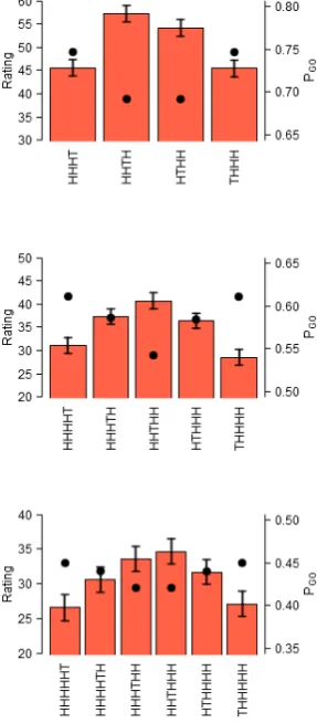
Figure 3. Bars show mean likelihood ratings for exact strings of heads (H) and tails (T)

which contain a single oddball, as part of a global sequence of coin tosses. (A) Estimates for

4-item strings as a part of a global sequence of 20 tosses. (B) Estimates for 5-4-item strings as a part

of a global sequence of 30 tosses. (C) Estimates for 6-item strings as a part of a global sequence

of 40 tosses. Error bars show standard error of the mean. Black circles show corresponding

values of probability of occurrence at least one (PGO) for each string. Strings with oddballs

closer to one end have higher rated likelihood, but lower PGO.

Hahn and Warren (2009) suggested that differences in PGO would be reflected in judgments only

when these differences were relatively large. In the absence of any information regarding what

constitutes a sufficiently large difference in PGO to be observable in judgments, this suggestion

risks being untestable. For example, the difference in likelihood ratings for HTHHTH (PGO = .40)

and HHHTHT (PGO = .45) is in the opposite direction to a considerable difference in PGO, but is

this difference sufficiently large for an influence of PGO to be expected? We return to this issue in

the General Discussion.

The question now becomes: if participants’ estimates bear little relation to PGO, then on

what information are they basing these estimates? In the Introduction, we noted three aspects of

(non-) representativeness that have been raised in previous theorizing: (1) relative proportion of

the two outcomes, (2) alternation rate, and (3) complexity. Below we consider each of these in

turn.

The first type of local non-representativeness comes from strings in which the overall ratio

of heads to tails deviates from 50:50. Here we quantify ‘proportion’ as the lower of either the

proportion of H in the string, or the proportion of T in the string. For example, proportion for

HHHT is .25, and for TTHHTT is .33. Thus, a proportion of .5 indicates equal numbers of H and

T, and a proportion of 0 indicates a string containing only one outcome.

The alternation rate heuristic refers to the proportion of transitions between adjacent items

in a string that involve an alternation between the binary outcomes, e.g., HHHTTT has an

alternation rate of 1/5 because it has one alternation out of five transitions, while HTHTHH has

an alternation rate of 4/5.

Finally, the complexity heuristic provides a more general conception of randomness

perception. The more complex a sequence appears to be (that is, the less structure it appears to

possess – which can be measured in terms of how hard it is to compress, remember, or

suggested based on concepts such as sequential independence, irregularity, entropy, and

incompressibility. It is beyond the scope of this article to evaluate these alternatives (for reviews,

see Falk & Konold, 1997; Nickerson, 2002). For the sake of simplicity, here we use Falk and

Konold’s (1997) Difficulty Predictor (DP), which provides a numerical measure of encoding

complexity, with higher values indicating greater complexity (for calculation details, see Falk &

Konold, 1997).

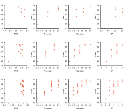
Figure 4. Scatterplots of mean likelihood ratings for 4-item strings (top row), 5-item strings

(middle row), and 6-item strings (bottom row) against: Probability of occurrence at least once

(PGO; first column); Lower of either the proportion of heads in the string, or the proportion of

(1997) Difficulty Predictor (DP; fourth column). In all panels, the data point closest to the

bottom left of the graph is for perfect repetitions of outcomes (e.g., HHHHH).

Figure 4 shows scatterplots of mean likelihood ratings for 4-, 5- and 6-item strings against

PGO, proportion, alternation rate, and DP. Looking at the plots for PGO, the point at the

bottom-left of each plot represents the string of perfect repetitions (e.g., HHHHH), which has the lowest

PGO by a considerable margin, and also received the lowest rating in each case. However, there is

no evidence of a positive correlation between PGO and ratings over the remaining strings. In

contrast, ratings over a range of strings appear to correlate with each of the representativeness

heuristic’s criteria. To analyze these data, we performed a regression analysis on the observed

likelihood ratings for the 4-, 5-, and 6-item strings, with the following predictor variables: (1)

PGO; (2) proportion; (3) alternation rate; (4) DP. We use a Bayesian regression analysis, so that

we can find evidence in favor of predictors being unable to predict the observed likelihood

ratings.

In our analysis, we fit all 16 regression models that exclude interaction terms (i.e., 4 models

with one predictor, 6 models with two predictors, 4 models with three predictors, 1 model with

all four predictors, and 1 model with no predictors). Our analysis gives us a marginal likelihood

for all 16 models. We use the marginal likelihoods for two purposes: First, to determine the most

likely model to have generated the observed likelihood ratings out of our candidate set of 16

models. Second, by averaging over different combinations of fitted models, we can also assess

the overall evidence for each predictor variable. In particular, we can compare the marginal

likelihood of the models that include each predictor with the marginal likelihood of the models

that exclude that predictor.

For 4-item strings, there are two models that parsimoniously predict the observed data,

alternation rate, and DP predictions, and performs slightly better (BF = 1.66) than the model that

includes the alternation rate and proportion predictors. The next best-fitting model includes all

four predictors, including PGO, but is 8.6 times less likely to have generated this observed data

than the best-fitting model. Averaging over all 16 models, our Bayes factor analysis of effects

indicates that models which include the PGO predictor are 8.7 times less likely to have generated

the observed data than the models that do not include PGO. Non-Bayesian regression found that a

model including only the proportion, alternation rate and DP predictors accounted for 97.7% of

the variance in mean ratings across the different strings.

For 5-item strings, the Bayesian analysis revealed that best-fitting model includes the

proportion and alternation rate predictors, being 4.6 times more likely than the next best model

(which also included the PGO predictor). Again, the inclusion of the PGO predictor leads to worse

fitting models, overall (BF=0.207). Non-Bayesian regression found that a model including only

the proportion and alternation rate predictors accounted for 94.0% of the variance in mean ratings

across the different strings.

For 6-item strings (our richest dataset), we see a similar result as for the 4-item strings. The

best-fitting model is one that includes the proportion and alternation rate predictors, but this

model provides an equivalent account (BF = 1.02) as one that also includes the DP predictor. The

next best-fitting model also included the PGO predictor, but was 10.3 times less likely to have

generated the observed likelihood ratings than the models that did not contain that predictor.

Averaging across models, those that included the PGO predictor were 14.5 times less likely to

have generated the data than the models that excluded PGO. Non-Bayesian regression found that a

model including only the proportion, alternation rate and DP predictors accounted for 92.0% of

the variance in mean ratings across the different strings.

In summary, participants’ probability judgments in Experiment 1 were essentially unrelated

heuristics relating to local representativeness, and a linear combination of these heuristics (but

not PGO) provided a good account of people’s performance. Returning to the potential

relationships between alternative norms and heuristic use, it seems clear from Experiment 1 that

participants do not use the alternative norms discussed by Hahn and Warren (2009) in place of

heuristics, nor do they appear to improve heuristic-based judgment by taking into account these

alternative norms. It is still possible that alternative norms explain the existence of heuristics. It is

also possible that although these alternative norms are a statistical reality, they are not related to

human judgment. We return to this issue in the General Discussion.

By asking participants to judge the likelihood of a given string appearing at least once in a

longer, finite global sequence, we ensured that PGO provided the normative basis for performance

in Experiment 1. So, for example, the correct response would be to provide a higher rating for

HHHT than HHTH, since HHHT has a higher value of PGO. And yet participants rated HHHT as

less likely than HHTH. It is clear, then, that participants’ estimates in Experiment 1 reveal

non-normative biases. Given that people do not follow the pattern of ratings predicted by this

alternative norm in a situation in which it is appropriate, it seems unlikely that their perception of

randomness in situations where using PGO is not appropriate (such as the procedure of Kahneman

& Tversky, 1972) is a consequence of an overgeneralization and misapplication of this metric.

3. Experiment 2

Although Experiment 1 showed clear effects, it has limitations. The task of predicting the

probability that a string occurs in a sequence at least once is both a difficult task about which to

reason, and is low in ecological validity. We also observed that several participants noted that

they thought that all strings had equal probability of occurrence, so gave similar ratings for all

options. In Experiment 2, participants made a series of binary choices between pairs of strings,

length. As each binary choice provides only a single bit of data, we decided to use only 5-item

strings in this study (rather than dividing participants between 4-, 5- and 6-item strings), in order

to maximize the number of comparisons for each pair.

We also provided a small amount of incentivisation for participants’ correct choices in

Experiment 2. This use of incentivization is potentially important. It has been argued that the

gambler’s fallacy is not really a fallacy, because participants who display it have the same chance

of winning as someone choosing randomly, showing the opposite (hot-hand) bias, or using any

other strategy. The probability of winning is always .5. While in Experiment 1 there was a

normatively correct pattern of responses (given by PGO), participants in this experiment made

judgments rather than choices, and hence in this case too they had no disincentive to show biases.

In Experiment 2, we used a task in which participants could do substantially better than winning

on 50% of trials, and in which their pay depended on whether they made the correct choice2.

3.1. Method

3.1.1. Participants. A total of 151 participants (47% female; median age = 31, range =

19-64; 48% university educated) were recruited from Amazon Mechanical Turk, as in Experiment 1.

No participant who had completed Experiment 1 completed Experiment 2. The experiment took

around 10 minutes to complete, and participants were paid $1.50, along with a

performance-related bonus which was $0.49 on average.

3.1.2. Design and Procedure. We created a subset of the set of 32 possible 5-item strings,

to exclude inverses (so the subset would not include both HHTTH and TTHHT), meaning there

were 16 items in the set, and thus 120 possible binary comparisons between non-identical

members of the 16-item subset.

Participants completed a series of 120 trials in which they chose the option from a pair of

General instructions introducing the idea of strings in sequences were the same as in Experiment

1. Additionally, participants were informed that they would win $0.01 on each trial that the string

they chose appeared in a virtual sequence of coin flips to be simulated at the end of the study, and

that the outcomes were independent in this regard:

It doesn't matter whether the other string appears or not - if the string you chose appears, you get a $0.01 bonus. If it does not, you get no bonus. So you should always choose the string you think is most likely to appear.

After reading the instructions, participants made the 120 binary choices, with one option on

the left of the screen, and the other on the right. Each option had a button beneath it labelled

‘THIS ONE’, and participants had to click one of the buttons to make their selection. They then

had to click a ‘NEXT’ button in the middle of the screen to continue to the next trial. For each of

the 120 binary choices, left-right position of the options was randomized for each participant, and

each option had a 50% chance of being presented as its inverse. So, taking HHTHH vs HHHHT

as an example of one of the 120 binary comparisons made, around a quarter of participants chose

between HHTHH and HHHHT; a quarter between TTHTT and HHHHT; a quarter between

HHTHH and TTTTH; and a quarter between TTHTT and TTTTH. As all theories under

consideration make identical predictions for all these pairs, the analysis treats them as a single

stimulus.

At the end of the experiment, a sequence of 20 random coin flips was generated for each

binary choice that the participant had made, and if the string that they had chosen appeared in the

sequence, their bonus was increased by $0.01.

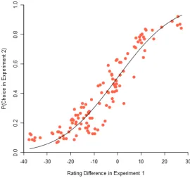
Figure 5. Proportion of binary choices made for item in Experiment 2 as a function of

differences in ratings between the two items in Experiment 1.

We first examined the congruency between the results of this choice Experiment and the

ratings in Experiment 1. A scatterplot showing the relationship between the difference in ratings

for a pair of strings in Experiment 1 and the probability of choosing a string in Experiment 2 is

shown in Figure 5. To analyse the data from Experiment 2, we ask how well we can predict

participants’ choices between each pair of strings, based on the various properties of each string.

For each pair of strings presented, we first evaluated the signed differences between the left and

right options in terms of the following variables: PGO, proportion, alternation rate, and DP. For

example, the string HHTHH has two alternations and HTHTH has four alternations, and so the

predictor value for this pair of strings would be +2, if HTHTH was the string on the right.

Participant choices were entered into a binary logistic regression (left option = 0; right option =

following variables: PGO, proportion, alternation rate, and DP. We conducted this regression

using a Bayesian approach so that we can quantify evidence for a null effect of predictors. The

model also assumed that each participant had their own set of coefficients for each prediction

(and an intercept), we assumed that individual parameter values were drawn from a

population-level Normal distribution. For example, we assumed that individual-participant alternation rate

coefficients, βALT, were drawn from a Normal distribution with mean, ΒALT, and standard

deviation, σALT. We focus our inference on the population-level mean parameters for each of the

predictor variables.

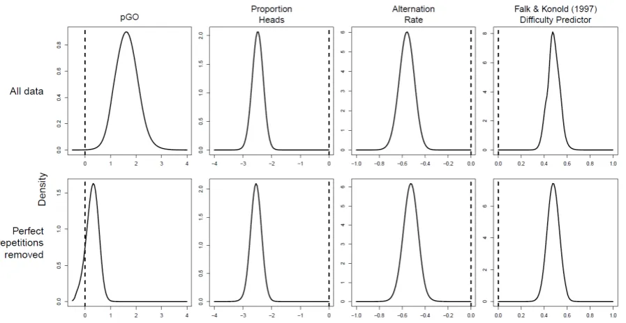
Figure 6. Posterior distributions for the coefficients for each of the predictor variables in our

Bayesian logistic regression analysis of Experiment 2, for the full dataset (top row), and for the

dataset excluding cases in which one of the items in the choice-pair was a string of perfect

repetitions (HHHHH or TTTTT). The dashed line at 0 in each panel is equivalent to a null-effect

of that predictor variable.

The five panels in the top row of Figure 6 plot the posterior distribution of the coefficients

for each predictor variable (i.e., the Β parameters). The posterior distribution represents the

made. Each of the five panels also contains a vertical dashed line at 0, which corresponds to a

‘null’ predictor variable.

The posterior distributions for the three local representativeness heuristic predictors

(proportion, alternation rate and DP) sit far from 0, suggesting that they are reliable predictors of

choice. The posterior for PGO has relatively little density at zero, suggesting that it is contributing

to participants’ choices, but its contribution is not as strong as for the heuristics.

Almost all support for the influence of PGO comes from trials in which one item of the pair

presented to participants is the string of prfect repetitions (HHHHH or TTTTT). Panels in the

bottom row of Figure 6 show the posterior distributions of coefficients for each predictor when

excluding trials containing perfect repetitions. As for the full dataset, these distributions reveal

strong support for an effect of proportion, alternation rate and DP. However, now the distribution

for PGO has considerable mass at zero, suggesting that it is unrelated to participants’ choices

when this small subset of extreme cases is removed.

There are numerous ways of quantifying the degree of support for these statements. For

example, if one has a prior likelihood that any given predictor variable was 0, then the ratio of the

prior and posterior likelihoods would yield a Bayes factor (cf. the Savage-Dickey test:

Wagenmakers, Lodewyckx, Kuriyal, & Grasman, 2010). Alternatively, one could construct a

95% credible interval for each predictor variable and determine whether zero (or a region

surrounding zero) fell within that interval (Kruschke, 2010). We prefer to abstain from either

approach, since it is clear from Figure 6 that our conclusions are robust to our choice of

inference.

4. Experiment 3

The results of Experiment 2 are strongly congruent with, and readily predicted by, those of

understand than Experiments 1 and 2, namely choosing which of two strings is likely to occur

first in a sequence of coin tosses. This makes the task particularly straightforward for

participants, and is not dependent on participants’ attention to the specifics of a string appearing

“at least once” in a sequence of coin flips.

We also ran Experiment 3 completely between-subjects, for two reasons. The first is that

providing probability ratings or binary choices for dozens of different sequences (as in

Experiments 1 and 2) is repetitive and effortful, and as such, participants may be inclined to use

heuristics that they would not use in shorter, less repetitive tasks. This could give the impression

that judgments are always driven by heuristics, when under normal circumstances they are not.

Secondly, the within-subjects design of Experiments 1 and 2 meant that participants saw a

number of strings of outcomes. Matthews (2013) has shown trial-to-trial context effects in

randomness judgments, and it is thus possible that our previous within-subjects designs produced

context effects which led to judgments that would not have been made in isolation.

We designed Experiment 3 to involve only a single trial per participant, combined with a

more readily understandable task, and some incentivization for normative choice. The rationale

was to use a simpler choice task, and a between-subjects design to trade off experimental power

with ecological plausibility. If, using a very different design, we found similar results, we could

be more confident that the phenomena observed here are not artifacts of the precise

implementation of the experiment. Thus, in Experiment 3, participants made a single binary

choice of which string they thought would occur first in a series of coin tosses. Clearly, with only

a single bit of information per participant, arranging for sufficient comparisons of every possible

pair of strings to allow robust statistical analysis would require an impractically large number of

participants. In Experiment 3 we therefore used a subset of all possible pairwise comparisons,

and recruited over three thousand participants online.

Experiments 1 and 2 were designed to make the use of PGO normative. However, despite our best

efforts they may not have been easy for participants to understand. Thus, in Experiment 3

participants were asked the simpler question of which of two strings they thought would appear

first if a coin were tossed repeatedly.

Making the task more ergonomic for participants adds a layer of normative complexity,

because although PGO is positively correlated with the actual probability of a string occurring

sooner, for binary choices, the correlation is not perfect. Notably, probability of occurring first in

sets of pairs violates transitivity; for example, for any string length k > 2 it is possible to find

another string of length k that has a higher probability of occurring first (see Gardner, 1974,

Penney, 1969).

Thus, the normative basis for behavior in Experiment 3 was different from that in

Experiments 1 and 2 (where PGO was the appropriate norm). We refer to the normative metric in

Experiment 3―the probability that string X will occur before string Y in a sequence of binary

outcomes―as Pfirst,X,Y. As Pfirst is not directly estimable by PGO, we include both measures as

potential alternative norms that participants might use. (We note that Pfirst, is a relatively unlikely

candidate, given the amount of experience required to learn the first occurrences of each possible

pair of strings, but as it is actually the normative baseline in this task, we include it for

completeness.) We examine whether these metrics describe behavior here, or whether instead

behavior was related to same representativeness properties that predicted behavior in

Experiments 1 and 2.

4.1. Method

4.1.1. Participants. A total of 3447 binary choices were collected. Participants completed

the choice task at the end of an unrelated 2-minute judgmental forecasting experiment (Reimers

www.maximiles.co.uk; see Reimers, 2009 for a brief introduction) for completing both

experiments. They were also paid a bonus of 10 maximiles points if their choice of string actually

came first in a sequence of random coin tosses that was simulated immediately after they made

their selection.

4.1.2 Design. Each participant made a choice between a pair of 5-item strings (see

Procedure). We used a subset of possible pairings, which covered all possible strings, but not all

possible pairings. As in Experiment 1, of the 32 different 5-item strings, two sets of 16 were

constructed. One set held all sequences that contained 2 or fewer heads. The other set held the

inverse strings that contained 2 or fewer tails. Within each set, all possible pairings of strings

were generated (120 per set). In other words, the two sets were identical except that in one set all

heads and tails had been swapped. All theories under consideration make identical predictions for

the two sets.

Participants were assigned a code based on the number of participants who had previously

started the experiment. This meant that across each set of 480 participants, all possible pairings

across the two sets were used as stimuli, with counterbalanced left-right positioning (although as

not all participants completed the experiment, there remained significant variation in the number

of participants for each pairing).

4.1.3. Procedure. Participants read the following instructions:

‘Next, we have a very quick two-choice question. If you get the right answer, you'll receive a bonus 10 maximiles points. Imagine a trusted friend is tossing a coin again and again, and is noting down each time whether it comes down heads (H) or tails (T). Your friend is going to carry on tossing the coin until a certain sequence of heads and tails comes up - for example it could be three heads in a row (HHH), or a tail followed by another tail followed by a head (TTH).

chosen sequence occurs first, you'll receive 10 bonus maximiles points. If the other sequence occurs first, you won't receive the bonus points (but you'll still get the points for the rest of the survey of course).

Repeatedly tossing a fair unbiased coin, which of the following precise sequences of heads and tails do you think will occur first?’

Below these instructions were two 5-item strings, one on the left and one on the right of the

screen. Participants clicked to indicate their choice. Immediately after making their choice,

participants saw a sequence of randomly simulated coin flips generated at the bottom of the

screen, which continued until one of the two strings presented in the choice came up. When this

happened, participants were informed whether they had won or not, and were debriefed.

4.2. Results and Discussion

To minimize the risk of repeat submissions, second and subsequent submissions from a

single email address or single IP address were deleted, leaving 3282 participants’ data.

Participants with response times of under 5 seconds (including reading the task instructions) were

also removed, leaving 3123 in the analysis. This gave a mean of 13.0 (SD = 2.27) participant

choices across the set of 240 pairs (min = 8, max = 18). For the analyses that follow our

dependent variable is the proportion of choices of the left-hand option, as presented on the

participant’s screen, as a function of the difference between the left- and right-hand options along

the dimensions of interest (such as Pfirst, alternation rate, etc).

Overall participants chose the string which actually did appear first on 51.5% of trials,

which was not significantly different from chance [binomial test, p = .11, 95% CI = (.497, .532)].

This suggests that whatever strategy or information participants were using, it was not helping

their overall performance.

Performance as a function of normativity and heuristics

normative choice, given by the difference between the actual probability of string X occurring

first and the probability of Y occurring first (Pfirst,X,Y – Pfirst,Y,X). For each pairing of strings we ran

100,000 simulated trials on which coin tosses were generated randomly until one of the strings

appeared. These simulated data were used to calculate an estimate of Pfirst,X,Y, and since either

string X or string Y must occur first we have Pfirst,Y,X = 1 – Pfirst,X,Y.

in Experiment 3, as a function of differences between the two strings in: (A) Hahn and Warren’s

PGO , (B) Hahn and Warren’s PGO, excluding streaks of the same outcome, (C) deviation from

equal proportions of H and T, (D) Falk and Konold (1997) Difficulty Predictor,(E)number of

alternations, and (F) actual probability of occurring first [Pfirst, based on a simulation of

100,000 sequences].

Figure 7A shows that there is a weak positive relationship between participants’ choices

and Hahn and Warren’s alternative norm, PGO. As in Experiment 2, the two clusters at the

bottom-left and top-right of this plot are the two sets of 15 pairs in which one of the pair is a

string of perfect repetitions (HHHHH or TTTTT). If these are removed only the central cluster

remains, and evidence for a positive correlation between PGO and choices disappears, as depicted

in Figure 7B.

Figures 7C-E show scatterplots of participants’ choices against the local representativeness

heuristics studied in Experiment 1: proportion, Falk and Konold (1997) Difficulty Predictor (DP),

and alternation rate. In contrast to Pfirst, each of these scatterplots shows evidence of a systematic

relationship between the heuristic and participants’ responses across the range of choices.Finally,

Figure 7F shows a scatterplot of participants’ choices against this normative metric, Pfirst. There is

Figure 8. Posterior distributions for each of the predictor variables in our Bayesian logistic

regression analysis of Experiment 3, for the full dataset (top row), and for the dataset excluding

cases in which one of the items in the choice-pair was a string of perfect repetitions (HHHHH or

TTTTT). The dashed line at 0 in each panel is equivalent to a null-effect of that predictor

variable.

To examine the relative predictive power of the different variables on participant choices,

we repeated the same regression analysis as in Experiment 2 with two differences. First, since

each participant contributed only one response, we could not estimate regression coefficients for

each individual. Second, we also included a predictor for the difference between values of Pfirst

for the left and right strings. The five panels in the top row of Figure 8 plot the posterior

distribution of each predictor variable, using the same format as in Figure 6.

This analysis revealed that the posterior distribution for the Pfirst predictor had considerable

mass at 0, suggesting that Pfirst does not reliably predict participants’ choices. However, the

coefficients for the three local representativeness heuristic predictors (proportion, alternation rate

and DP) have essentially no posterior density at 0, suggesting that they are reliable predictors of

The posterior for PGO follows a similar pattern to that in Experiment 2. There appears to be

some evidence for the predictive value of PGO (top row of Figure 8), but this conclusion rests

entirely upon choices between pairs that include strings of perfect repetitions (bottom row of

Figure 8).

In summary, as in Experiments 1 and 2 participants’ choices were well-explained by the

application of local representativeness heuristics based on a small number of properties of a

string’s outcomes. For the whole dataset, there was some evidence to suggest an effect of the

alternative norm represented by PGO, but this was entirely driven by the fact that participants

rarely chose the string of perfect repetitions (HHHHH) when it was presented in the choice pair,

and this string has the lowest PGO (but of course it also has the lowest values of proportion,

alternation rate, and DP). When choices involving the string of perfect repetitions are excluded,

PGO is unrelated to choices. This stands in contrast to the heuristic measures, which reliably

predict participants’ choices across the whole dataset. Non-Bayesian logistic regression revealed

that the best-fitting model including only the proportion, alternation rate and DP predictors

explained 51% of the variance in participants’ proportional choice of each item in a pair of

options across the whole dataset.

These findings suggest that, while proportion, alternation and DP all penalize HHHHH,

they do not do so as strongly as participants, and it is this additional variance that is picked up by

PGO. However, this isolated success does not provide a strong case for a more general role of PGO

in participants’ randomness perception. An alternative view is that the failure of heuristics to

accurately model the size of the disadvantage for HHHHH reflects our assumption of a linear

effect of each heuristic. For example, in terms of alternation rate, the linear assumption means

that the difference between strings containing zero versus one alternation is considered

psychologically equivalent to the difference between strings containing one versus two

more salient than the 1–2 difference.

Figure 9. Scatterplot showing the proportion of participants choosing each string from a pair in

Experiment 3, as a function of the difference in likelihood ratings in Experiment 1 (left panel, r =

.67) and choices in Experiment 2 (right panel, r = .77)

Consistency with Experiment 1

Finally, we compared participants’ behavior in Experiment 3 with the choices that would

be predicted on the basis of the results of Experiment 1. If decisions were based on similar

processes in the two different tasks, as we predict, then we should expect to observe a strong

positive correlation between them. The scatterplot in Figure 9 shows the proportion of choices of

the left-hand option in Experiment 3 as a function of predictions based on the ratings in

Experiment 1 and choices in Experiment 2. The clear positive relationships suggest that

participants in Experiment 3, as a group, performed comparably to, and consistently with, those

in Experiments 1 and 2. Bearing in mind that responses in Experiment 3 were binary choices, and

some cells contained only 8 of these binary observations, the strength of these correlations seem

consistent with the idea that participants used very similar strategies across all three experiments.

Experiments 1 and 2 were the result of the surface characteristics of any one of the experiments.

5. General discussion

A pervasive view in the cognitive psychology literature is that people’s perception of

randomness is fundamentally biased: that judgments regarding the relative likelihood of different

strings of events reflect non-normative heuristics relating to the local representativeness of those

strings. Much of the basis for this reasoning comes from a very small number of exemplars used

by Kahneman and Tversky (1972). Consequently, these studies lack the sensitivity to distinguish

between judgments based on the use of representativeness heuristics, versus judgments based on

environmental experience of real patterns that, in some cases (but not all), coincide with

representativeness. This latter view suggests that randomness perception is fundamentally a

property of (unbiased) experience that can then be over-extended to situations in which this

experience is no longer a good guide to classifying sequences of outcomes as random or not. In

other words, judgments in a particular task may be based on (or sensitive to, or correlated with)

alternative norms developed on the basis of related prior experience

Three experiments assessed participants’ sensitivity to alternative norms, by measuring

likelihood ratings (Experiment 1) or incentivized choices (Experiments 2 and 3) for different

strings of heads and tails that could occur in a sequence of coin tosses. In none of these cases did

participants’ behavior show sensitivity to the appropriate normative metric. Instead, behavior in

all experiments was best explained by a small number of properties relating to local

representativeness: the proportion of each outcome, alternation rate, and local complexity. The

fact that the different methodologies of the three experiments gave similar results suggests that

participants use very similar approaches to assess the relative probability of a particular series of