Methods for improving the accuracy of automated NDE systems

Methods for improving the accuracy of automated NDE systems

Jonathan Riise1, Lance Farr2, Martyn Lindop2, Gareth Pierce1, P. Ian Nicholson2, and Ian Cooper2

1_{Centre for Ultrasonic Engineering, Department of Electrical and Electronic}

Engineering, University of Strathclyde, Glasgow G1 1XW, UK. Email: [email protected]

2_{TWI Technology Centre (Wales), Harbourside Business Park, Harbourside Road, Port}

Talbot, SA13 1SB, UK

Abstract

Automated inspection systems using twin six-axis industrial robots have been available for a number of years, including the IntACom system at TWI Wales. Utilising phased array ultrasonic probes to quickly inspect complex geometries, the IntACom system is now routinely used in various inspections of composite components. In the present work we introduce a number of methods for improving and quantifying the accuracy of an automated inspection system. The key challenges are identified and addressed through a number of methods including calibration procedures and interfacing multiple sensors with industrial robots for Non Destructive Evaluation (NDE) purposes. The authors also introduce a novel method for improving the Tool Centre Point (TCP) calibration of an industrial robot when the tool is an ultrasonic phased array probe. Experimental trials show that the average positioning error is less than 0.5mm using this new method. Keywords: Calibration, Robotic Inspection, Ultrasonic Testing (UT), IntACom, Phased Array

1

Introduction

Most inspection systems rely on Off-Line Path Planning (OLP) which utilises Computer-Aided Design (CAD) models of components to generate trajectories for the robots to fol-low. This approach increases the flexibility of the system and reduces setup time for new parts but relies on the accuracy of calibrations to be successful. As a result, one of the fundamental challenges has been improving the positional and orientation accuracy of these emerging inspection systems.

Figure 1: The IntACom robot inspection cell at TWI Wales.

This paper presents some of the ways the research undertaken at TWI Wales has helped to overcome these problems by integrating sensors and developing calibration methods. Section 2 will discuss the relevance of coordinate reference frames and how the calibration of each of these can be carried out. Section 3 introduces a novel method for calibration a phased array probe with respect to a robot’s reference frame based on ultrasonic measurements. Section 4 will present experimental results and discuss the ob-tainable accuracy and repeatability.

2

Reference Frame Calibration

Wrist Frame{W}

World Frame{O}

Tool Frame{U}

Part Frame{B}

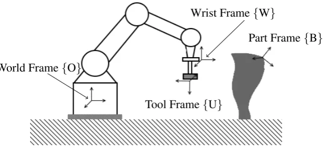
Figure 2: Schematic of the different reference systems used in a robotic inspection system.

From an operator’s perspective, the aim of any inspection is to be able to identify the position and size of any indications within a part relative to some datum on the part. This is achieved through Eq. 1 where eachT represents a 4x4 homogeneous matrix (see Equation 2). In Equation 2, Ris a 3x3 rotation matrix and t is the 3D position vector, (x,y,z)T. The geometrical transformation between the tool frame,{U}and the wrist frame (TU

W) as well as the transformation between the part frame{B}and world frame{O}(TBO)

must be found prior to inspection. The aim of path planning is to determine a number of positions and orientations that the tool,{U}must be moved to in order to inspect areas of interest. These initial calibrations are crucial as they determine the accuracy with which indications will be recorded. The world-to-part calibration is commonly referred to as the base calibration while the wrist-to-tool calibration is simply known as the tool calibration.

T_BU =T_WU ∗T_OW ∗T_BO (1)

H=

R t 0 1

(2)

2.1

Part Positioning

Figure 3: Scan Control 2D scanner from MicroEpsilon [7].

2.2

Tool Calibration

The IntACom system uses a squirter system setup which provides the benefit of immer-sion scanning without the need for an immerimmer-sion tank as water jets couple the ultrasound to the component. A tool calibration is needed to be able to determine where in 3D space ultrasound was emitted from and in which direction it travels. As a number of probes can be used on the system, a quick and reliable Tool Centre Point (TCP) calibration is needed to ensure positional accuracy over time. The TCP calibration of a robot can be carried out manually by driving the centre of a tool to the same point from at least four different orientations (referred to as the ”spike method”). Though this may be sufficient for some applications, this approach does not lend itself to ultrasonic probes for a number of reasons. First of all, the centre of the array is located behind a matching material and is not directly accessible. Secondly, when using squirter systems, the nozzle itself hinders access to both the transducer casing and phased array probe. Furthermore manual meth-ods are prone to operator error and variability and thus a automated method which utilises ultrasonic measurements is guaranteed to be both more accurate and reliable. An auto-matic calibration routine can also be carried out as part of an inspection plan to validate the gathered results and to determine long-term reliability.

2.2.1 Hand-eye calibration of a phased array probe

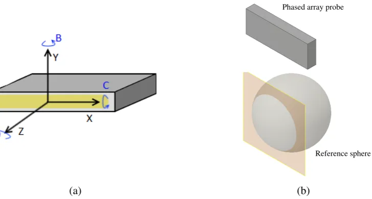
The key contribution of this paper is to adapt the method presented in [6] to the calibration of a phased array probe with respect to the wrist of an industrial robot. A phased array probe can be considered to have an internal coordinate system wherein the Z-direction is normal to the probe face, the X-direction is parallel to the active aperture of the probe (along the array) and the Y-direction is along the travel path of the probe during inspection (see Figure 4a). This coordinate system is not necessarily aligned with the coordinate system of the robot wrist and thus both a translation (Xu,Yu,Zu) and a set of rotations

(Au,Bu,Cu) need to be found. To find the centre and orientation of the probe, a reference

sphere is ultrasonically imaged from at least six different robot orientations, as shown in Figure 4b. This provides a single-step calibration of the location and orientation of the TCP coordinate system. The orientation of the probe is then optimised by monitoring the reflected signal from a flat reference sample.

(a)

Phased array probe

Reference sphere

(b)

Figure 4: (a) Coordinate system of a linear phased array probe. Each of the blue letters denotes rotation about that axis. (b) Imaging a reference sphere to find the TCP. At each robot pose, the phased array produces an imaging plane (in yellow) which is reflected off the sphere.

calibration problem AX=XB, where X is the unknown transformation and A and B are different tool poses. To be able to reconstruct the same point in space from a number of orientations, a reference sphere with a known diameter was used as this can be ultra-sonically imaged from any direction. This also overcomes the 2D limitation of a phased array probe as the 3D sphere centre position can be calculated For each position, a recon-structed probe Y-coordinate can be found by measuring the radius of the circle formed when intersecting a sphere with a plane (see Figure 4b) and calculating the distance to the sphere centre. After calculating these positions from the ultrasonic data, the following relationship between a point in the robot’s reference frame (Po = (Xo,Yo,Zo)T) and the

phased array’s reference frame (Pu =(Xu,Yu,Zu)T) is the following: Po = TWO·TUW·Pu

(with reference to Figure 2). For a number of robot poses, the following set of equations can be generated:

     

    

Po =TWO1·TUW·Pu1

Po =TWO2·TUW·Pu2

.. .

Po =TW iO ·TUW·Pui

(3)

If the physical location of the sphere (Po) remains constant in the robot’s reference frame,

then Equation 3 can be rearranged to give (for eachj6=i):

T_{W j}O ·T_UW·P_uj =T_{W i}O ·T_UW·P_ui (4)

2.2.2 Imaging the surface of a sphere

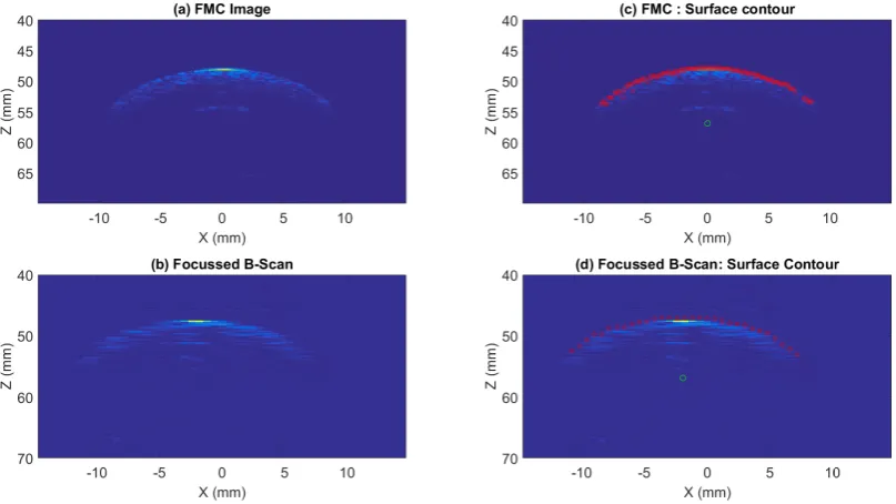
The passive aperture of the probe is defined by the width of the elements and causes the beam to have a three dimensional volume below the probe unlike a laser beam which can be considered to be nearly two dimensional. Hence, the reflection and beam-spread of the sound wave, coupled with effects from the water jet can causes a large uncertainty in the determination of the probe centre. As the measured sphere centre is sensitive to any error in the determination of the circle radius, efforts were made to obtain the best possible ultrasonic image. It was found that using the Full-Matrix Capture (FMC) method and subsequent Total Focussing Method (TFM) for image generation gave the most accurate results, as shown in Figure 5.

Figure 5: The difference in imaging resolution between the FMC method and a standard focussed B-Scan. The accuracy of the extracted surface contour is higher when using FMC as shown by the red marks. Each green marker shows the centre of the circle formed by the ultrasonic beam.

For each robot pose, a FMC dataset is acquired and a TFM image is formed. The image is then analysed to find the surface of the sphere by applying a threshold to the pixels in each row. A curve is then fitted to the points for removing outliers and a circle is fitted the boundary points to obtain the centre of the circle. As the true radius of the sphere is known, the distance from the centre of the circle to the centre of the sphere can be calculated.

2.2.3 Accuracy enhancements

in water and the diffraction limit. After the one-step process has been completed, the orientation can further be adjusted by moving the ultrasonic probe over a flat surface. The probe is then rotated about angle C in both directions and the maximum intensity of the reflections is found. Next a B-scan is analysed such that the front-wall reflection from the flat surface is straight (angle B). Finally, the probe is scanned across a line reflector (such as a straight edge or wire) to provide any corrections to the angle A.

3

Experimental Results

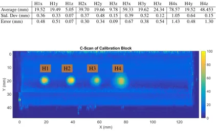
A series of experiments were carried out to determine the accuracy of the previously described calibration method. To determine the accuracy, a reference block measuring 40.0 x 130.0 x 60.0mm containing four flat bottomed holes of nominal diameter 5mm at depths of 4.98mm, 9.87mm, 24.88mm and 49.90mm was scanned using the IntACom system. The reported position of each of the indications will be a function of both the robot’s accuracy as well as the TCP and base calibrations. The position of the reference block with respect to the robot base was measured using a laser profiler. Afterwards, the block was ultrasonically scanned using a calibrated phased array probe. To ensure the TCP calibration was correct, the scan was performed five times with the probe’s Y direction travelling in the direction of the longest axis of the block and as well as five times perpendicular to the longest axis. The average location, standard deviation and error from true position of the indications are shown in Table 1.

Table 1: Results from 10 scans of a calibration block in two perpendicular directions. The error is given as the difference in position between the measured and actual value.

H1x H1y H1z H2x H2y H3z H3x H3y H3z H4x H4y H4z

Average (mm) 19.52 19.49 5.05 39.70 19.66 9.78 59.33 19.62 24.34 78.57 19.52 48.453 Std. Dev (mm) 0.36 0.33 0.07 0.37 0.48 0.15 0.39 0.52 0.12 1.05 0.64 0.15 Error (mm) 0.48 0.51 0.07 0.30 0.34 0.09 0.67 0.38 0.54 1.43 0.48 1.30

H1 H2 H3 H4

Data was gathered using the IntACom acquisition software, a 5MHz, 64el probe and a Micropulse 5PA instrument from PeakNDT. The pitch of the probe was 0.6mm and a sub-aperture of 16 elements was used to create a uniform beam profile. As shown in Figure 6, the deepest defect is not resolved very clearly. Excluding this last defect, the average errors for X,Y, and Z are∆X = 0.49mm,∆Y = 0.31mm and ∆Z = 0.23mm demonstrating that the system is capable of achieving better than 0.5mm positional accu-racy on average. It should be noted that this is over a small volume and at low speeds (under 200mm/s) and that further work is needed to quantify this error within the robot’s working envelope .

4

Conclusions and Further Work

Several robot inspection systems have been on the market for a number of years, but few papers have been published discussing the positional accuracy in the context of NDE. This work has shown that defects can be located with sub-mm positional accuracy. In the future the authors hope to further develop the calibration routine and determine the accuracy for larger volumes and the effects of using complex paths.

5

Acknowledgements

The authors would like to thank Mark Sutcliffe and Carmelo Mineo for their support. This work was undertaken as part of the RCNDE EngD programme with funding from EPSRC, grant reference number 1797043 and support from TWI Ltd.

References

[1] I. Cooper, I. Nicholson, D. Liaptsis, B. Wright, and C. Mineo, “Development of a fast inspection system for complex aerospace structure,” in6th International Symposium on NDT in Aerospace, no. November, Madrid, 2014, p. 1.

[2] C. Mineo, C. MacLeod, M. Morozov, S. G. Pierce, R. Summan, T. Rodden, D. Ka-hani, J. Powell, P. McCubbin, C. McCubbin, G. Munro, S. Paton, and D. Watson, “Flexible integration of robotics, ultrasonics and metrology for the inspection of aerospace components,” in AIP Conference Proceedings, vol. 1806, no. 1, 2017, p. 020026. [Online]. Available: http://aip.scitation.org/doi/abs/10.1063/1.4974567

[3] E. Cuevas and S. Hern´andez, “Robot-based solution To Obtain an Automated , Inte-grated And Industrial Non-Destructive Inspection Process,”6th International Sympo-sium on NDT in Aerospace, no. November, pp. 12–14, 2014.

[5] M. Morozov, J. Riise, R. Summan, S. Pierce, C. Mineo, C. MacLeod, and Brown R.H., “Assessing the Accuracy of Industrial Robots through Metrology for the en-hancement of Automated Non-Destructive Testing,” in IEEE International Confer-ence on Multisensor Fusion and Integration for Intelligent Systems, vol. 44, 2016, pp. 335–340.

[6] S. Yin, Y. Ren, Y. Guo, J. Zhu, S. Yang, and S. Ye, “Development and calibration of an integrated 3D scanning system for high-accuracy large-scale metrology,” Measure-ment: Journal of the International Measurement Confederation, vol. 54, pp. 65–76, 2014. [Online]. Available: http://dx.doi.org/10.1016/j.measurement.2014.04.009