Manuel Chiach´ıo1, Juan Chiach´ıo2, Shankar Sankararam3, and John Andrews4
1,2,4Resilience Engineering Research Group, Faculty of Engineering, University of Nottingham, NG7 2RD, Nottingham, UK
[email protected] [email protected]
3NASA Ames Research Center, Intelligent Systems Division, Moffett Field, CA, 94035-1000, USA
ABSTRACT
This paper presents a mathematical framework for model-ing prognostics at a system level, by combinmodel-ing the prognos-tics principles with the Plausible Petri nets (PPNs) formal-ism, first developed in M. Chiach´ıoet al.[Proceedings of the Future Technologies Conference, San Francisco, (2016), pp. 165-172]. The main feature of the resulting framework re-sides in its efficiency to jointly consider the dynamics of dis-crete events, like maintenance actions, together with multiple sources of uncertain information about the system state like the probability distribution ofend-of-life, information from sensors, and information coming from expert knowledge. In addition, the proposed methodology allows us to rigorously model the flow of information through logic operations, thus making it useful for nonlinear control, Bayesian updating, and decision making. A degradation process of an engineer-ing sub-system is analyzed as an example of application us-ing condition-based monitorus-ing from sensors, predicted states from prognostics algorithms, along with information coming from expert knowledge. The numerical results reveal how the information from sensors and prognostics algorithms can be processed, transferred, stored, and integrated with discrete-event maintenance activities for nonlinear control operations at system level.
1. INTRODUCTION
In prognostics, the integration of the predicted information at a system level encompasses two distinct research challenges. First is about predicting the change in system performance and remaining life estimation through an adequate combina-tion of the degradacombina-tion rates and states of health of individ-ual components. Second, and perhaps most important, to
Manuel Chiach´ıo et. al. This is an open-access article distributed under the terms of the Creative Commons Attribution 3.0 United States License, which permits unrestricted use, distribution, and reproduction in any medium, pro-vided the original author and source are credited.
integrate system-level nonlinearities and uncertainties with the predicted information from prognostics. Here, system-level nonlinearities are understood as uncertain environmen-tal elements that affect the system operation irrespectively of the component-wise state of health or degradation, like intervention processes (e.g. maintenance actions), resource availability,ad hocsynchronization of components, influence of expert knowledge, etc. In the literature, the majority of prognostics research to date has been focused on individual components, and determining theirend-of-life(EOL) and re-maining useful life(RUL), e.g.: (Chiach´ıo, Chiach´ıo, Saxena, & Goebel, 2016; Zio & Peloni, 2011; My¨otyri, Pulkkinen, & Simola, 2006; Saha, Celaya, Wysocki, & Goebel, 2009; Daigle & Kulkarni, 2013). Besides, few attempts can be encountered describing system-level prognostics methodolo-gies. Generally, these attempts provide the EOL of a sys-tem based on its constituent components and how they inter-act, like in Gomez, Rodrigues, Galvo, and Yoneyama (2013), where a system-level approach was developed using fault tree analysis from the RUL of individual components. Daigle, Bregon, and Roychoudhury (2014) provided a distributed ar-chitecture to model system-level prognostics based on the concept of structural model decomposition whereby the so-lution of independent local prognostics subproblems were in-tegrated to obtain prognostics at system-level. Liu, Xu, Xie, and Kuo (2014) studied multi-component maintenance mod-els with economic dependence for components that degrade in a continuous manner. More recently, an analytic frame-work has been provided in (Khorasgani, Biswas, & Shankarara-man, 2016) for combining the degradation rate of individual components to predict the variation in system performance over time. Nonetheless, to the authors best known, holistic methodologies for prognostics with integration of system or sub-system level nonlinearities and uncertainties, still remain missing in the literature.
mod-eling prognostics at a system level by using Petri nets (PNs) (Petri, 1962). In particular, the newly developed Plausible Petri nets(PPNs) (Chiach´ıo, Chiach´ıo, Prescott, & Andrews, 2016) are used to integrate uncertain information about the system, like the probability density function (PDF) of EOL for multiple components, information from sensors, expert knowledge, etc., with the dynamics of discrete events like system-level health indicators, maintenance activities, resour-ce availability, to cite but any. Consequently, the approach has the advantage of being able to integrate by first time informa-tion from prognostics (e.g. EOL, RUL, etc.), with decision making aspects like go/no-go decisions for maintenance ac-tions. Moreover, the uncertainty is intrinsically accounted for in PPNs, since its formulation stems from combining the in-formation theory principles with the PNs technique, as will be shown further below.
To exemplify some of the problems that can be solved by the proposed methodology, several toy examples are formulated through a set of PPN architectures. Next, the framework is tested using a numerical example to model decision-making over a two-component engineering system under degradation using prognostics information, expert knowledge, and main-tenance actions, which is just some of the challenges faced in system-level prognostics applications using PPNs.
The remainder of the paper is organized as follows. Section 2 briefly overviews basic concepts about prognostics and PNs before introducing the fundamentals of PPNs. The PPNs for-malism as well as their execution semantics, are succinctly described in §3. A set of examples of PPN architectures for system-level prognostics are provided and discussed in §4. Section 5 illustrates our approach through a numerical exam-ple about two-component degrading system. Finally, Section 6 gives concluding remarks.
2. BASIC CONCEPTS
2.1. Foundations of prognostics
Prognostics is concerned with predicting the future health state of engineering systems or components given current de-gree of wear or damage, and, based on that, estimating the remaining time beyond which the system is expected not to perform its intended function within desired specifications (Chiach´ıo, Chiach´ıo, Sankararaman, Saxena, & Goebel, 2015). In the PHM community, the aforementionedremaining time
is typically referred as RUL. The potential of prognostics in positively contributing to safety and cost relies in its capac-ity to provide anticipated information about an anomalous or faulty condition. This information can be used for risk re-duction in go/no-go decision, cost optimization through the scheduling of maintenance as-needed, and improved asset avail-ability.
Broadly, formal approaches for prognostics fall into three
pri-mary categories (Javed, Gouriveau, & Zerhouni, 2017; Kho-rasgani et al., 2016): (1) data driven techniques, (2) model based, and (3) hybrid approaches, depending on how the fault propagation process is modeled. Irrespective of the type of modeling approach chosen for prognostics, two main distinct research problems can be devised: (i) theestimation prob-lem, which determines the current state of health of the sys-tem, and (ii) the failure prediction problem, by which the EOL and RUL can be obtained from predictions of the future state of the system`-steps forward in time in absence of new observations. For the estimation problem, the component, sub-system, or system state of health or degradation is typ-ically assumed to be represented using a stochastic variable
xk. This state variable evolves over timekfollowing a
spe-cific dynamic equation given in state-space form (Chiach´ıo et al., 2015; Zio & Peloni, 2011), as follows:
xk=fk(xk−1,uk,vk,θ) (1a)
yk=hk(xk,uk,wk,θ) (1b)
whereuk ∈Rnu is an input vector,y
k ∈Rny is a
measure-ment vector, andvk ∈ Rnv andw
k ∈ Rnw are uncertain
variables introduced to account for the model error and mea-surement error, respectively. The functionsfkandhkare
pos-sibly nonlinear functions for the state transition evolution and observation equation, respectively. This model is sequentially evaluated at every time stepk, and produces updated informa-tion about the system statexkas long as new measurements
are available. Next, prognostics algorithms can be employed to project the state predictions into future in absence of new observations. Then, by having defined a failure regionF, the EOL can be obtained as the earliest time indexk+`, ` >1 when the event[xk+`∈ F]occurs. It can be computed as:
EOLk =infk+`∈N:`>1∧I(F)(xk+`) = 1 (2)
whereI(F)is an indicator function that maps a given point in thex-space to the Boolean domain{0,1}, such thatI(F)= 1 ifx ∈ F, and0 otherwise. The RUL predicted from time kcan be straightforwardly obtained from EOLk as RULk =
EOLk−k. Note that due to the probabilistic nature of the state
variable given byxk, then EOL and RUL are also described
as stochastic variables.
Finally, it is important to remark that in this work, the focus is not on predicting the EOL or RUL of a system as a probabil-ity, but on methodology that integrates EOL and RUL within an asset management framework at a system level, as will be described next.
2.2. Basis of Petri nets
p1
p2
[image:3.612.317.556.141.267.2]p3 2 t1
Figure 1. Example of Petri net of three places and one transi-tion.
A place represents a particular state of the system or activity being modeled (e.g. considering health management model-ing, places can be used to indicate the current state of a com-ponent or sub-system, if the performance of this comcom-ponent or sub-system is currently being tested by a maintenance team to determine its state, or if any maintenance activity is cur-rently in progress). Places are temporarily visited bytokens, the abstract moving units of a PN. The distribution of tokens over the PN at a specific time of execution is referred to as
marking, which is expressed as a vector indicative of the state of the PN. The transitions are responsible of the dynamic be-havior of the PN, and enable the system to move from one state to another. For example, a component wear process is one of such processes which can be reflected using a tran-sitions (Andrews, Prescott, & De Rozi`eres, 2014). In graphi-cal representation, places are typigraphi-cally expressed using circles while transitions are drawn as bars or boxes. Arcs are labeled with their correspondingweights, non-negative integer values indicating the amount of parallel arcs (1 by default). Figure 1 is provided to serve as illustrative example of a PN of three places (p1,p2,p3), and one transition (t1).
From a mathematical point of view, a PN can be defined as an ordered 6-tupleNas follows (Murata, 1989):
P,
P,T,E,M0,D,W (3)
whereP ∈ Nnp andT ∈
Nnt denote the set ofn
p places
andnttransitions of the PN respectively,M0 ∈ Nnpis the
initial marking, andD ∈ Rnt is the non-negative vector of
switching delays of the transitions (0 by default). The set
E ⊂ Nnp ×
Nnt represents the edges (also referred to as
arcs), which are expressed through ordered pairs of nodes to indicate the connections between places and transitions, i.e.E⊆(P×T)∪(T×P). As mentioned above, each edge has assigned a weight (1by default) within the set of weights
W.
At a certain statek, the PN dynamics can be described through an algebraic equation defined by:
Mk+1=Mk+ATuk (4)
whereuk is thefiring vector atk, a nt-dimensional vector
of Boolean values whose elements are obtained according to the firing rule.A ∈ Nnt×np is theincidence matrixof the
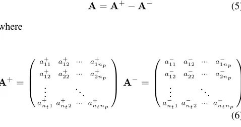
graph, whose elements are the result of subtracting the for-ward(A+)andbackward(A−)incidence matrices respec-tively, as follows:
A=A+−A− (5)
where
A+ =
a+11 a + 12 ··· a
+ 1np
a+12 a + 22 ··· a
+ 2np
..
. . ..
a+nt1a +
nt2 ··· a+ntnp
A−=
a−11 a
−
12 ··· a
−
1np
a−12 a
−
22 ··· a
−
2np
..
. . ..
a−nt1a
−
nt2 ··· a−ntnp
(6)
The elementa+ijfrom Eq. (6) represents the weight of the arc
from transitiontito output placepj, whereasa−ijis the weight
of the arc to transitiontifrom input placepj,i = 1, . . . , nt,
j = 1, . . . , np. If transition ti is activated at state k, then
ui,k ∈ukis modified according to thefiring rule, which can
be expressed as follows:
ui,k=
(
1, if M(j)>a−ij ∀pj ∈ •Pti
0, otherwise (7)
whereM(j)∈ Nis the marking for placepj, and•Pti
de-notes the set of places that belong to the preset of transi-tionti, i = 1, . . . , nt. For example in the PN from Fig. 1, •P
t1={p1, p2}.
Note that by means of PNs and their marking, the behavior of complex engineering systems can be described in terms of discrete system states and their changes over time. The following rules summarize the algebra of PNs as explained above:
1. Transitions always consume from all the input arcs at the same time and produce from all out-coming arcs the same amount;
2. Transitionti is enabled if every input placepj from its
preset•Ptiis marked with at leasta − ijtokens;
3. An enabled transitiontiwill fire once the delay timeτi∈
Dhas passed;
4. After firing, transitiontiremovesa−ijtokens frompj, and
addsa+ijtokens to eachj-th output place ofti.
p(1N) p(1S)
p(2N) a−11
a0
11− a0
11+
a+12 t1
[image:4.612.82.255.71.199.2]Preset oft1 Postset oft1
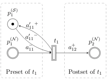
Figure 2. Illustration of a sample PPN with two numerical places (p(1N),p
(N)
2 ), one symbolic place (p (S)
1 ), and one tran-sition (t1).
based on sequences of Boolean operations. Thus, over the last decades, researchers have enhanced the original PNs to han-dle (1) uncertainty (Konar & Mandal, 1996; Looney, 1988; Cao & Sanderson, 1993; Bugarin & Barro, 1994; Zhou & Zain, 2016; Cardoso, Valette, & Dubois, 1999), and (2) con-tinuous variables to efficiently reproduce the hybrid aspect of systems without the need of employing complex graphs (David, 1997; Antsaklis, 2000; J´ulvez, Di Cairano, Bempo-rad, & Mahulea, 2014; Vazquez & Silva, 2015; Silva, 2016). Plausible Petri Nets (PPNs) (Chiach´ıo, Chiach´ıo, Prescott, & Andrews, 2016) can be classified as one of these variants of the PNs developed to better reproduce the nature of engi-neering systems, hence giving partial response to the referred drawbacks, as will be shown next.
3. PLAUSIBLEPETRINETS(PPNS)
Plausible Petri nets (PPNs) are a class of PNs recently de-veloped by the authors, which are based on a combination of discrete and continuous numerical processes whose val-ues may be uncertain (plausible). Two interacting subnets form the PPN graph: 1) a symbolic subnet, where the to-kens are objects in the sense of integer moving units, as in classical PNs (Petri, 1962), 2) a numerical subnet, where tokens arestates of information 1. The resulting framework
is a hybrid variant of PNs where the sets of nodes{P,T}
are partitioned into two disjoint subsets, namely numerical and symbolic, which are denoted using superscripts(N)and (S), respectively. In particular, the set of placesPare par-titioned into subset P(N) ∈
Nnp andP(S) ∈
Nn
0
p, such
that P(N)∪ P(S) = P, and P(N) ∩P(S) = ∅. Super-scriptsnp, n0p represent the number of numerical and
sym-bolic places, respectively. Analogously, transitionsTare par-titioned into numerical transitionsT(N)∈Nnt and symbolic
transitions T(S) ∈ Nn0
t, where T(N) ∪ T(S) = T, and
1A state of information can be described by a set of numerical values about a
state variable, along with a mapping over them that assigns each numerical value with itsrelative plausibility(Tarantola & Valette, 1982; Rus, Chi-ach´ıo, & ChiChi-ach´ıo, 2016).
T(N) ∩T(S) =6 ∅. In this case, nt, n0tdenote the number
of numerical and symbolic transitions, respectively. Observe that those transitions that belong toT(N)∩T(S)are referred to asmixed transitions(Chiach´ıo, Chiach´ıo, Prescott, & An-drews, 2016).
In PPNs, the referred states of information about a system state variablexk ∈ X are denoted by fp(xk)and ft(xk)
for numerical places and transitions, respectively. In prac-tical terms, these states of information can be understood as probability density functions (PDFs) except for a normalizing constant. Thus, the markingMkof a PPN at a certain timek
consists in a combined vectorMk =
M(kN),M(kS), where
M(kN)andM(kS)are column vectors of normalized PDFs and integer values, respectively. Moreover, as in classical PNs, there exist arc weights for the symbolic places, denoted by a0ij+, a0ij− ∈W(S) ⊂N, whereby the incidence matrixA(S)
can be obtained by Eq. (5). The arc weights for the numeri-cal places are denoted bya+ij, a−ij ∈W(N)⊂R+, such that
A(N) =
a+ij
−
a−ij
, and i = 1, . . . , nt, j = 1, . . . , np,
wherent, np represent the amount of numerical transitions
and numerical places of the PPN, respectively. Note that the arc weights from the symbolic subnet, e.g. (a0
11−)are dif-ferentiated from the numerical ones using an accent (0). In graphical representation, numerical nodes are represented us-ing double line, whereas sus-ingle line is used for the rest. A PPN model is shown in Fig. 4 for illustration purposes. The dashed rectangles shown in Fig. 4 are to highlight the preset and postset oft1.
3.1. Execution semantics
As stated in the last section, the marking at timekof PPNs consists of both types of information given byM(kN)for the numerical places, andM(kS)for the case of symbolic places. The marking evolution of the symbolic subnet corresponds to the state equation of a PN (Murata, 1989) (recall Eq. [4]). However, the evolution ofM(kN)relies on anad hoc informa-tion flow dynamics based on two basic operainforma-tions (Chiach´ıo, Chiach´ıo, Prescott, & Andrews, 2016): theconjunctionand
fa(x)
fb(x)
f(x) = (fa∧fb) (x) =1
α fa(x)fb(x)
µ(x)
α: constant
x
fa(x)
fb(x)
f(x) = (fa∨fb) (x) =1
β fa(x) +fb(x)
, β: constant
[image:5.612.129.488.81.199.2]x
Figure 3. Illustration of the conjunction (left) and disjunction (right) of two arbitrary states of information, namelyfa(x)and
fb(x).
details.
From this standpoint, the dynamics of PPNs is formulated un-der the adoption of the following rules (Chiach´ıo, Chiach´ıo, Prescott, & Andrews, 2016):
1. An input arc from placep(jN) to transitionti ∈ T(N)
conveys a state of information given bya−ij fpj∧fti
(xk),
which remains inp(jN)after transitiontihas fired;
2. Transitionti ∈ T(N)produces to an output arc a state
of information given by a+ij fti ∧ f
•P
ti(xk), where f•Pti(x
k) denotes the resulting density from the
dis-junction of the states of information of the preset ofti. As
stated in Fig. (3), the normalized version off•Pti(x k)
can be obtained as:
f•Pti(x k) =
1 β f
p1+fp2+· · ·+fpm
(xk) (8)
whereβis a constant, andp1, . . . , pm∈ •Pti ⊂P
(N);
3. After firing numerical transitionti, the state of
informa-tion resulting in placep(jN)from the postset ofti, is the
disjunction of the state of informationfpj(x
k)(the
pre-vious state of information), anda+ij fti∧f•Pti(xk)(the
information produced after firing transitionti). In
math-ematical terms:
fpj(x
k+1) =
fpj ∨a+
ij fti∧f
•P
ti(xk) (9)
The rules given above are sufficient to explain the informa-tion flow dynamics of PPNs. Notwithstanding, observe that they are mostly based on conjunction of states of information which requires the evaluation of normalizing constants in-volving an intractable integral. Also, note that there are situa-tions where the conjunction is conducted using density func-tions which are not completely known, perhaps because they are defined trough samples. Particle methods (Arumlampalam, Maskell, Gordon, & Clapp, 2002; Doucet, De Freitas, & Gor-don, 2001) can be used in these cases to circumvent the
eval-uation of the normalizing constant with a feasible computa-tional cost. In particle methods, a set ofNsamplesx(n) N
n=1 with associated weights
ω(n) N
n=1are used to obtain an ap-proximation for the required density function [e.g. fa ∧
fb(x)], as follows:
fa∧fb(x)≈ N
X
n=1
ω(n)δ x−x(n)
(10)
whereδis the Dirac delta andx(n)∼ fa∧fb(x). The
parti-cle weightω(n)represents the likelihood value ofx(n), and is representative of the plausibility ofx(n)when it is distributed according to fa∧fb(x). It can be evaluated for the case of
X being a linear space as follows (Tarantola & Mosegaard, 2007):
ω(n)= fa(x (n))f
b(x(n))
PN
n=1fa(x(n))fb(x(n))
(11)
A pseudocode implementation to obtain a particle approxi-mation from the conjunction fa∧fb(x), is provided in the
Appendix as Algorithm 1.
3.1.1. Firing rule
In PPNs, any transitionti ∈Tis fired at timekif the delay
time has passed and:
1. Every symbolic place from the preset ofti has enough
tokens according to their input arc weight, as in classical PNs;
2. Each of the conjunction of states of information between ftiandfpj
k is possible, wherep
(N)
j belongs to the preset
ofti;
3. Conditions (a) and (b) are both satisfied when ti is a
mixed transition, i.e.ti∈(T(S)∩T(N)).
Note from Condition (b) that a conjunction, e.g. fpj
k ∧f ti
k
(xk),
is possible if fpj
k ∧ f
ti
k
(xk) 6= ∅ (Tarantola & Valette,
p(1N)
p(1S) Working condition
p(2N)
p(3N)
Buffer
p(2S)
Maintenance needed
a−12
a−
11
a0
11−
a0
12+
a+ 13
t1
(a)
p(1N)
p(1S) Working condition
p(2N)
p(3N)
Buffer
p(2S)
Maintenance needed
a−11
a011
−
a0
12+
a+ 13
t1
a−12
a120 −
a+23
t2
[image:6.612.86.532.92.262.2](b)
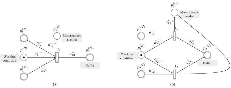
Figure 4. Plausible Petri nets of the examples given in §4.1.
involved in a conjunction is the homogenous density (also referred to as “non-informative density”)µ(xk)of the state
space of considerationX, then the conjunction is always pos-sible (Tarantola & Valette, 1982; Chiach´ıo, Chiach´ıo, Prescott, & Andrews, 2016), thus Condition (b) is automatically ful-filled. This argument is important in terms of using PPNs in practical applications, as will be demonstrated in next section.
4. SYSTEM LEVELPHMBYPPNS
In this section, a set of PPN sample architectures are provided to illustrate how our PPNs can be used for decision mak-ing at a system level in applications where information from prognostics along with other sources of information (like ex-pert knowledge, sensors, etc.) may coexist, as usual in prac-tice. The examples have been kept as simple as possible since they are mostly intended to serve as guideline to built more complex PPNs. Moreover, the examples provide represen-tative architectures whereby to conceptualize the proposed PNN methodology in a prognostics and health management context.
4.1. Integrative decision making for multi-component prog-nostics
A couple of PPN architectures are exemplified here for mod-eling decision making aspects in presence of multiple infor-mation about the EOL from different components of an en-gineering system. Figure 4 shows two PPNs of three numeri-cal{p(1N), p(2N), p3(N)}and two symbolic{p1(S), p(2S)}places, along with one mixed transitiont1(two transitions for Fig. 4b). This example assumes that numerical placesp(1N)andp
(N) 2 enclose uncertain information about the EOL of two com-ponents or sub-systems, which is expressed through a PDF denoted by fEOL1 andfEOL2, respectively. Transition t
1 is defined based on condition (Chiach´ıo, Chiach´ıo, Prescott, &
Andrews, 2016) using an indicator function for the state space that assigns a value of 1 when the expected value of EOL reaches a specific threshold denoted by ∈ R, and0
other-wise, as indicated in Table 1. Provided that place p(1S) has one token (assumed thata011 = 1in this example), then, ac-cording to the firing rule given in §3.1.1, transitiont1is acti-vated once the expected EOL from both components or sub-systems has reached the threshold value(not necessarily at the same time), whereupon the system turns to a “mainte-nance needed” state. The resulting information is collected in place p(3N) which acts as a buffer of information. This buffer can be used for diagnostics purposes since it collects a weighted distribution of plausible EOL values from the two-component system, conditioned toE(EOLk)> . As stated
by the execution semantics of PPNs (refer to §3.1), the result-ing PDF inp(3N)can be described as:
fp3 = a
+ 13 a−11+a−12
a−11fEOL1+a−12fEOL2
(12)
Note from the last equation that whena−11=a−12=a+13= 1,
then fp3 = 1
2
fEOL1 +fEOL2, an averaged sum of both
PDFs of EOL.
p(1N)
p(1S)
p(2N)
Expert information
p(3S)
p(3N)
a−11
a011
−
a+ 13
a0
13+
t1
a−
12
a
+ 23
a0
23−
t2
(a)
p(1S) Working condition
p(1N)
p(5S) Component
being repared
p(2N) Buffer
p(3S)
Maintenance needed
a−11
a0
11−
a+ 12
a0
13+
a0
15+
t1
p(4S) Available engineers
a0
23−
a024
−
a0
25+
t2
[image:7.612.99.546.87.283.2](b)
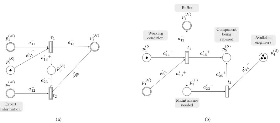
Figure 5. Illustration of the exemplified PPN architecture explained in §4.2 (left) and §4.3 (right).
4.2. Combining expert knowledge and prognostics mea-sures
In this section, an example of PPN is provided which includes information about the PDF of EOL of a component or sub-system, along with information coming from expert knowl-edge. Figure 5a illustrates the PPN consisting of three numer-ical places, two symbolic places, and two transitions. Let us now assume that the numerical placep(1N)comprises the PDF of EOL of a component given byfEOL, whereasfp3=∅,
ini-tially. Next, the proposed PPN architecture also encompasses information from one expert in placep(2N), which is repre-sented by a PDF given byfExpert (e.g.fExpert can be a
uni-form PDF of EOL representing an interval of possible values of EOL). As in the last example, transitiont1is defined based on condition, such that it is fired if the uncertainty2 of the PDFfEOLreaches or exceeds a specific threshold value. Ift
1 is fired, then placep(2S)receives a token that enables the
infor-2For example by calculating the differential entropy of the PDF of EOL
(Chiach´ıo, Beck, Chiach´ıo, & Rus, 2014; Chiach´ıo, Chiach´ıo, Prescott, & Andrews, 2016)
mation from the expert to be transferred to placep(3N). Note that through this exemplified PPN, a decision making process can be modeled about the adoption of information from an expert if the uncertainty about the EOL is higher than a cer-tain valueξ. For example, this can be as a consequence of a faulty sensor, or a perturbed prognostic estimation. The re-sulting information inp(3N) includes the PDFfEOL coming
fromp(1N)and that from the expert, as follows:
fp3 = a
+ 13 a−11+a−12
a−11fEOL1+a−
12f
Expert
(13)
If required, higher relevance can be conferred to the expert in-formation by increasing the weighta−12with respect toa−11. Fi-nally, observe that the PDFfp3 can be further used in an
op-erational context (e.g., for diagnostics), as was described in last section.
Table 1. Description of the transitions of the PPN shown in Figs. 4a, 4b, 5a, and 5b.
Reference Transition Type Condition State of information
Fig. 4 t1 Mixed C1=
xk∈ X :EfEOL1(xk)6 ft1 ∼IC1(xk)
t2(Fig.4b) Mixed C2=xk∈ X :EfEOL2(xk)6 ft2 ∼IC2(xk)
Fig. 5a t1 Mixed C1=
xk∈ X :EfEOL(xk)6 ft1 ∼IC1(xk)
t2 Mixed None (homogeneus) ft2 ∼µ(xk)
Fig. 5b t1 Mixed C1=
xk∈ X :EfEOL(xk)6 ft1 ∼IC1(xk)
[image:7.612.108.504.608.721.2]4.3. Integration of prognostics and resource availability
This example illustrates the case of a decision making pro-cess, like activation of a maintenance action, taken after the PDF of EOL has reached a certain valueas in §4.1, except that in this case it occurs contingent upon availability of en-gineers. Fig. 5b shows the idealized system using a PPN of two numerical places, four symbolic places, one mixed tran-sition, and one symbolic transition. Numerical placep(1N)is assumed to represent the PDFfEOL of a component. As in
the example shown in Fig. 4a,t1is fired once the expecta-tion offEOL has reached the thresholdprovided that p(S)
1 has enough amount of tokens according toa011−, which for the sake of illustration, is assumed to bea011 = 1. Next, let us also assume that symbolic transitiont2represents the acti-vation of the maintenance activity (an actiacti-vation delayτ can be assigned tot2(Andrews et al., 2014), although this infor-mation is irrelevant here). Observe that whent1is fired, then t2 will be activated if the number of available engineers is higher or equal toa024−. In such case,p
(S)
5 is marked, then the system turns to “component being repaired” state.
5. NUMERICAL EXAMPLE
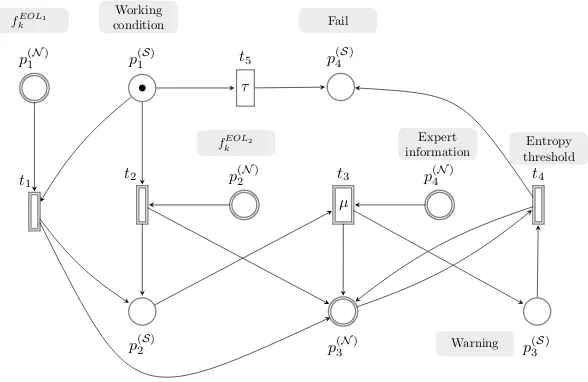
The PPN framework presented above is exemplified here us-ing a numerical example to illustrate some of the advantages of using PPNs for integration of prognostics at a system level. In this example, a self-managed two-component system is modeled through a PPN which comprises uncertain informa-tion about the EOL of two degrading components acting in series, along with expert knowledge about the whole system’s EOL. Figure 6 illustrates the idealized system model through a PPN of four numerical places, four symbolic places, and
five transitions. Noisy measurements about the components’ state of degradation are assumed to be available, whereby an estimation of the EOL can be obtained, provided that there exists a specified degradation threshold, and an appropriate prognostics algorithm to make predictions (see for example (Chiach´ıo, Chiach´ıo, Shankararaman, & Andrews, 2017)). Let us denote by EOL(kj) ∈ X ⊂ R+ a stochastic variable
corresponding to the EOL of thej-th component,j = 1,2, which evolves over timek ∈ Nfollowing a dynamic
equa-tion EOL(kj)=hk(x EOLj
k−1, θj)given by:
EOL(kj)=e−θjkEOL(j)
k−1+vk (14)
whereθj is an uncertain decay parameter whose values are
modeled as a Gaussian centered at 0,006 and 0,008 forj = 1,2,respectively, and 100% of coefficient of variation in both cases. The termvk represents a measurement error which
is assumed to be modeled as a zero-mean Gaussian density function with standard deviation given by σv = 5. In the
PPN, the mixed transitionsti,i = {1,2,4} are defined by
condition, thus their states of information can be expressed using Diract Delta density functions (Tarantola, 2005), i.e., fti(EOL
k) ∼ ICi(EOLk). Henceforth, their activation is
prescribed for the stochastic variable EOL(kj)on fulfilling the condition EOL(kj)∈ Ci, such that:
C1=EOLk∈ X :Efp1(EOLk)6 (15a)
C2=EOLk∈ X :Efp2(EOLk)6 (15b)
C3=EOLk∈ X :H(EOLk)> ξ (15c)
where = 20andξ = 5. In (15c), H denotes the differ-ential entropy of EOLk, that can be obtained by evaluating
p(1N) p (S) 1
p(2S)
p(2N)
p(3N)
t1
p(4S)
p(3S)
t2 fEOL1
k
fEOL2 k
Working
condition Fail
p(4N) Expert
information thresholdEntropy
Warning
µ
t3 t4
[image:8.612.169.463.500.691.2]τ t5
0 5 10 15 20 25 30
k
0 20 40 60 80 100 120 140
E
O
L
kThreshold
(²2= 20)(a)
0 5 10 15 20 25 30
k
0 20 40 60 80 100 120 140
E
O
L
kThreshold
(²2= 20) [image:9.612.101.514.86.310.2](b)
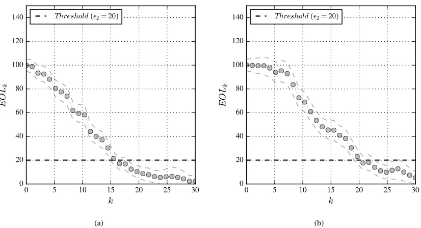
Figure 7. Plots of the evolution over time of the states of information about the stochastic variable EOL(kj)for components j= 1,2(panels [a] and [b], respectively) from the Plausible Petri net of the example given in §5. The expectation of the states of information is represented using gray circles. The dashed lines represent the5th-95th probability band.
1/2ln [(2πe)var(EOL
k)]as a measure quantifying the
uncer-tainty of EOLk. The initial marking of the numerical places
is given byfp1
0 ∼ N(100,5),f
p2
0 ∼ N(100,5),f
p3
0 = ∅, andfp4 =U[18,22]. The latter represents expert knowledge
about EOL, which is given by a uniform PDF defined over the interval[18,22].
Initially atk = 0, the system starts in the “working condi-tion” state represented by one token atp(1S), thusM(0S) = (1,0,0,0)T. Once any of the expected values of the predicted EOL of components 1 and 2 (represented in placep(1N)and p(2N), respectively) has reached the threshold value , then transitions t1, t2 (not necessarily both nor simultaneously) produce one token top(2S)which enables transitiont3 to be fired, whereupon the expert information about system’s EOL enters into play and is transferred top(3N). Next, the system turns to a “warning” state, and a decision is made conditioned upon: 1) the quality of the information given byfp3
k , and 2)
the total time spent by the system under no failure states. The differential entropy (DE) is used in this example as a qual-ity indicator of the information in place p(3N), so that the transitiont4is activated if the DE offkp3 is higher than the
thresholdξ = 5. In such case, the system turns to “inspec-tion needed” state, otherwise the system remains in “warn-ing” mode. In this example, the time spent by the system in performing transitiont5(which corresponds to an activation time given byτ) is assumed to represent a scheduled periodic maintenance activity such that ifk > τ, then the system
di-rectly turns to the “maintenance needed” condition irrespec-tive of the component’s degradation state nor their predicted EOL.
For the numerical evaluation of the PPN in Fig. 6, the ex-ecution semantics rules (recall §3.1) along with Eq. (4), are applied in confluence with the firing rule for the system state evolution described through the markingMk. The algorithm
for particle approximation of conjunction of states of infor-mation described in the Appendix, has been applied using N = 1000. Note that the disjunction of states of information
Table 2. Summary of the discrete events taking place when running the PPN shown in Fig. 6. The second and third col-umn show the symbolic marking and firing vector, respec-tively.
Time M(kS) uk Event
k= 0 (1 0 0 0) (0 0 0 0 0) – k= 1 (1 0 0 0) (0 0 0 0 0) –
..
. . ..
[image:9.612.337.535.573.720.2]0 5 10 15 20 25 30 35 40
EOL
(3)k
[image:10.612.67.269.76.287.2]0.000
0.002
0.004
0.006
0.008
0.010
0.012
0.014
0.016
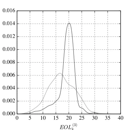
Figure 8. Kernel density estimates of the state of information about EOL in placep(3N)fork= 17andk>18(darker gray color).
can be straightforwardly evaluated using samples by just join-ing the samples from the component-wise density functions, and affecting their particle weights using an appropriate nor-malizing constant so as to obtain a bone fide density. Figure 7 shows the results for the two-components’ EOL (from places p(1N) andp
(N)
2 ) for time indexesk = 0tok = 30. Note from Fig. 7 that component 1 first reaches the threshold, i.e., the expectation of EOL(1)k first reaches the value = 20at k = 16. Next, transitiont3 is enabled and the information coming from the expert is aggregated top(3N)atk= 18. Fig-ure 8 shows the resulting PDF inp(3N) before and after the information from the expert was incorporated. Observe the influence of the expert knowledge in terms of gain of infor-mation, which makes the distribution of plausible EOL val-ues being more concentrated around the recommended valval-ues from the expert, namely [18,22]. Notwithstanding, the DE of the resulting state of information given byfp3 atk
> 18is higher thanξ= 5, then the system finally turns to the ”main-tenance needed” state. A summary of the results for the sym-bolic subnet of the PPN model is provided in Table 2.
This example illustrates that uncertain information about the EOL of different components along with information from experts, can be integrated into a system level model for prog-nostics and decision making. The numerical results confirm that system non linearities, apart from that attributable to the stochastic variable EOLk, can be taken into account.
Exam-ples of the referred non linearities are: ad hocsynchronies between components, user-defined time to failure, resources availability, etc., which makes our PPNs useful for prognos-tics and health management at a system level.
6. CONCLUSIONS
This paper presented a novel prognostics methodology to in-tegrate information from prognostics with decision making aspects at a system level using Plausible Petri nets. The ap-proach has the advantage of addressing the prognostics prob-lem as a unified system-level approach where multiple sources of uncertain information can be integrated with discrete-events, conferring high versatility to better reproduce real-world prob-lems of prognostics without the need of using extremely com-plex nets, as usual when adopting other formalisms. Further research is needed to investigate suitable PPN architectures to better integrate the influence of intervention activities within the predicted state of health at a system level.
ACKNOWLEDGMENT
This work was supported by the Lloyd’s Register Founda-tion, a charitable foundation in the UK helping to protect the life and property by supporting engineering-related ed-ucation, public engagement, and the application of research.
REFERENCES
Andrews, J., Prescott, D., & De Rozi`eres, F. (2014). A stochastic model for railway track asset management.
Reliability Engineering & System Safety,130, 76–84. Antsaklis, P. J. (2000). Special issue on hybrid systems:
the-ory and applications a brief introduction to the thethe-ory and applications of hybrid systems.Proceedings of the IEEE,88(7), 879-887.
Arumlampalam, M., Maskell, S., Gordon, N., & Clapp, T. (2002). A tutorial on particle filters for on-line nonon-linear/non-Gaussian Bayesian tracking. IEEE Transactions on Signal Processing,50(2), 174–188. Bugarin, A. J., & Barro, S. (1994). Fuzzy reasoning
sup-ported by Petri nets.IEEE Transactions on Fuzzy Sys-tems,2(2), 135–150.
Cao, T., & Sanderson, A. C. (1993). Variable reasoning and analysis about uncertainty with fuzzy Petri nets. In
International conference on application and theory of Petri nets(p. 126-145).
Cardoso, J., Valette, R., & Dubois, D. (1999). Possibilistic Petri nets. IEEE Transactions on Systems, Man, and Cybernetics, Part B: Cybernetics,29(5), 573-582. Chiach´ıo, J., Chiach´ıo, M., Sankararaman, S., Saxena, A.,
& Goebel, K. (2015). Prognostics design for struc-tural health management. InEmerging design solutions in structural health monitoring systems(pp. 234–273). IGI Global.
Chiach´ıo, M., Beck, J. L., Chiach´ıo, J., & Rus, G. (2014). Approximate Bayesian computation by Subset Simulation. SIAM Journal on Scientific Computing,
36(3), A1339-A1358.
(2016). An information theoretic approach for knowl-edge representation using Petri nets. InProceedings of Future Technologies Conference, 6-7 December 2016, San Francisco(pp. 165–172).
Chiach´ıo, M., Chiach´ıo, J., Saxena, A., & Goebel, K. (2016). An energy-based prognostic framework to predict evo-lution of damage in composite materials. In Struc-tural health monitoring (shm) in aerospace structures
(p. 447-477). Woodhead Publishing-Elsevier.
Chiach´ıo, M., Chiach´ıo, J., Shankararaman, S., & Andrews, J. (2017). A new algorithm for prognostics using Subset Simulation. Reliability Engineering & System Safety, in press.
Daigle, M., Bregon, A., & Roychoudhury, I. (2014). Dis-tributed prognostics based on structural model decom-position.IEEE Transactions on Reliability,63(2), 495-510.
Daigle, M., & Kulkarni, S. (2013). Electrochemistry-based battery modeling for prognostics. InProceedings of the annual conference of the prognostics and health man-agement society, 2013(Vol. 1, p. 249-261).
David, R. (1997). Modeling of hybrid systems using continu-ous and hybrid Petri nets. InProceedings of the seventh international workshop on Petri nets and performance models (PNPM’97), 1997.(pp. 47–58).
Doucet, A., De Freitas, N., & Gordon, N. (2001). An introduction to sequential Monte Carlo methods. In A. Doucet, N. De Freitas, & N. Gordon (Eds.), Se-quential Monte Carlo methods in practice(pp. 3–14). Springer.
Gomez, J., Rodrigues, L., Galvo, R., & Yoneyama, T. (2013). System level rul estimation for multiple-component systems. InProceedings of Annual Conference of the Prognostics and Health Management Society (p. 74-83).
Javed, K., Gouriveau, R., & Zerhouni, N. (2017). State of the art and taxonomy of prognostics approaches, trends of prognostics applications and open issues towards matu-rity at different technology readiness levels. Mechani-cal Systems and Signal Processing,94, 214–236. J´ulvez, J., Di Cairano, S., Bemporad, A., & Mahulea, C.
(2014). Event-driven model predictive control of timed hybrid Petri nets. International Journal of Robust and Nonlinear Control,24(12), 1724-1742.
Khorasgani, H., Biswas, G., & Shankararaman, S. (2016). Methodologies for system-level remaining useful life prediction. Reliability Engineering and System Safety,
154, 8-18.
Konar, A., & Mandal, A. K. (1996). Uncertainty management in expert systems using fuzzy Petri nets. IEEE Trans-actions on Knowledge and Data Engineering,8(1), 96-105.
Liu, B., Xu, Z., Xie, M., & Kuo, W. (2014). A value-based preventive maintenance policy for multi-component
system with continuously degrading components. Re-liability Engineering & System Safety,132, 83-89. Looney, C. G. (1988). Fuzzy Petri nets for rule-based
deci-sion making.IEEE Transactions on Systems, Man, and Cybernetics,18(1), 178–183.
Murata, T. (1989). Petri nets: Properties, analysis and appli-cations.Proceedings of the IEEE,77(4), 541-580. My¨otyri, E., Pulkkinen, U., & Simola, K. (2006). Application
of stochastic filtering for lifetime prediction.Reliability Engineering and System Safety,91(2), 200–208. Petri, C. A. (1962). Kommunikation mit automaten
(Unpub-lished doctoral dissertation). Institut fr Instrumentelle Mathematik an der Universitt Bonn.
Rus, G., Chiach´ıo, J., & Chiach´ıo, M. (2016). Logical infer-ence for inverse problems.Inverse Problems in Science and Engineering,24(3), 448-464.
Saha, B., Celaya, J. R., Wysocki, P. F., & Goebel, K. F. (2009). Towards prognostics for electronics compo-nents. InAerospace conference, 2009 ieee(pp. 1–7). Silva, M. (2016). Individuals, populations and fluid
approx-imations: A Petri net based perspective. Nonlinear Analysis: Hybrid Systems,22, 72–97.
Tarantola, A. (2005). Inverse problem theory and methods for model parameters estimation. SIAM.
Tarantola, A., & Mosegaard, K. (2007).Mapping of probabil-ities, theory for the interpretation of uncertain physical measurements. Cambridge University Press.
Tarantola, A., & Valette, B. (1982). Inverse problems = quest for information. Journal of Geophysics, 50(3), 159-170.
Vazquez, C. R., & Silva, M. (2015). Stochastic hybrid ap-proximations of Markovian Petri nets. IEEE Trans-actions on Systems, Man, and Cybernetics: Systems,
45(9), 1231–1244.
Zhou, K.-Q., & Zain, A. M. (2016). Fuzzy Petri nets and industrial applications: a review. Artificial Intelligence Review,45(4), 405-446.
Zio, E., & Peloni, G. (2011). Particle filtering prognostic es-timation of the remaining useful life of nonlinear com-ponents. Reliability Engineering and System Safety,
96(3), 403–409.
BIOGRAPHIES
work, Manuel worked as guest scientist at world-class univer-sities and institutions, like Hamburg University of Technol-ogy (Germany), California Institute of TechnolTechnol-ogy (Caltech), and NASA Ames Research Center (USA). This research has led to several publications in highly ranked journals. It has been awarded by the National Council of Education of Spain through one of the prestigious FPU fellowships, by the An-dalusian Society of promotion of the Talent, by the European Council of Civil Engineers (ECCM) with the Silver Medal prize in the 1st European Contest of Structural Design (2008), and also by the Prognostics and Health Management Society with a Best Paper Award in 2014. Prior to joining the Univer-sity of Granada in 2011, Manuel worked as a consultancy en-gineer for four years in top enen-gineering companies in Spain.
Juan Chiach´ıois a Research Fellow in Infrastructure Asset Management in the Resilience Engineering Research Group at the University of Nottingham (UK). He received his PhD in Structural Engineering (international mention) in 2014 by the University of Granada, Spain. In addition, he holds a MSc in Structural Engineering (2011) and a MSc in Civil Engineer-ing (2007), both by the University of Granada. His research is focused on translating reliability and prognostics methods into the life-cycle analysis of structural and infrastructural systems subjected in-service degradation. This research has led to several publications in highly ranked journals, a best-paper award and nominations in major conferences, and it has been awarded by the Spanish National Council of Educa-tion through one of the FPU annual fellowships, by the An-dalusian Society of Promotion of Talent, by the Prognostics and Health Management Society with a Best Paper Award, and by the European Council of Civil Engineers. In addi-tion, his work has attracted the interest of world-class insti-tutions for collaborative research, like the Prognostics Center of Excellence of NASA, the California Institute of Technol-ogy, and the Hamburg University of Technology (Germany). His current research at the University of Nottingham deals with the development of a Bayesian prognostics framework for infrastructure asset management, under EPSRC project titled ”Whole-life cost assessment of novel material railway drainage systems (EP/M023028/1)”.
Shankar Sankararamanreceived his B.S. degree in Civil Engineering from the Indian Institute of Technology in Ma-dras (2007) and later, obtained his Ph.D. in Civil Engineer-ing from Vanderbilt University, Nashville, Tennessee, U.S.A. in 2012. His research focuses on the various aspects of un-certainty quantification, integration, and management in dif-ferent types of aerospace, mechanical, and civil engineering systems. His research interests include probabilistic
meth-ods, risk and reliability analysis, Bayesian networks, system health monitoring, diagnosis and prognosis, decision-making under uncertainty, treatment of epistemic uncertainty, and mul-tidisciplinary analysis. He is a member of the Non-Determi-nistic Approaches (NDA) technical committee at the Ameri-can Institute of Aeronautics, the Probabilistic Methods Tech-nical Committee (PMC) at the American Society of Civil En-gineers (ASCE), and the Prognostics and Health Manage-ment (PHM) Society. Currently, Shankar is a researcher at NASA Ames Research Center, Moffett Field, CA, where he develops algorithms for uncertainty assessment and manage-ment in the context of system health monitoring, prognostics, and decision-making. He has been recently named as virtual member of the Resilience Engineering Research Group, Uni-versity of Nottingham (UK).
APPENDIX
Pseudocode implementation to obtain particles from the con-junction of two arbitrary states of informationfa(x)andfb(x).
Algorithm 1Particle approximation of conjunction of states of information
Inputs: N, fa(x), fb(x){number of particles and states of
infor-mation}
Outputs:
n
x(n), ω(n)oN
n=1
,wherex(n)∼(f
a∧fb)(x)
Begin
1: Samplen x˜(an),ω˜(an)
oN
n=1fromfa(x) 2: Setx(n)←˜x(n)
a , n= 1, . . . , N
3: Setωˆ(n)←fb x(n)
, n= 1, . . . , N {unnormalized weights}
4: Normalize weightsω(n)← ωˆ(n) PN
n=1ωˆ(n)