Published online in Wiley InterScience (www.interscience.wiley.com). DOI: 10.1002/jnm
Parallel preconditioners for high order discretizations arising from
full system modeling for brain microwave imaging
Marcella Bonazzoli
1∗, Victorita Dolean
1,2, Francesca Rapetti
1, Pierre-Henri Tournier
31Laboratoire J.A. Dieudonn´e, University of Nice Sophia Antipolis, Parc Valrose, 06108 Nice Cedex 02, France. E-mail: [email protected], [email protected], [email protected]
2Department of Mathematics and Statistics, University of Strathclyde, Glasgow, UK. E-mail: [email protected]
3INRIA Paris, Alpines, and UPMC - Univ Paris 6, CNRS UMR 7598, Laboratoire Jacques-Louis Lions, France. E-mail: [email protected]
SUMMARY
This paper combines the use of high order finite element methods with parallel preconditioners of domain decomposition type for solving electromagnetic problems arising from brain microwave imaging. The numerical algorithms involved in such complex imaging systems are computationally expensive since they require solving the direct problem of Maxwell’s equations several times. Moreover, wave propagation problems in the high frequency regime are challenging because a sufficiently high number of unknowns is required to accurately represent the solution. In order to use these algorithms in practice for brain stroke diagnosis, running time should be reasonable. The method presented in this paper, coupling high order finite elements and parallel preconditioners, makes it possible to reduce the overall computational cost and simulation time while maintaining accuracy.
Copyright c2016 John Wiley & Sons, Ltd.
Received . . .
KEY WORDS: Schwarz preconditioners; high order finite elements; edge elements; time-harmonic Maxwell’s equations; microwave imaging.
1. INTRODUCTION
The context of this work is the solution of an inverse problem associated with the time-harmonic Maxwell’s equations, with the aim of estimating the dielectric properties of the brain tissues of a patient affected by a brain stroke. Strokes can be cast in two major categories, ischemic (80% of strokes) and hemorrhagic (20% of strokes), which result in opposite variations of these dielectric properties. In the following, we briefly describe this particular medical context as well as the application motivating the numerical model.
During an ischemic stroke the blood supply to a part of the brain is interrupted by the formation of a blood clot inside a vessel, while a hemorrhagic stroke occurs when a blood vessel bursts inside the brain. It is essential to determine the type of stroke in the shortest possible time in order to start the correct treatment, which is opposite in the two situations: in the first case the blood flow should be
∗Correspondence to: Laboratoire J.A. Dieudonn´e, University of Nice Sophia Antipolis, Parc Valrose, 06108 Nice Cedex 02, France. E-mail: [email protected].
Contract/grant sponsor: French National Research Agency (ANR), project MEDIMAX; contract/grant number: ANR-13-MONU-0012.
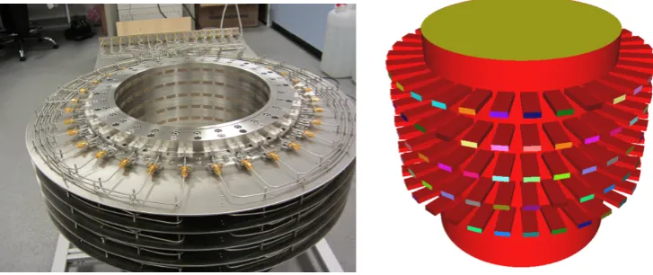
Figure 1. Imaging chamber of EMTensor (no copyright infringement intended).
restored, while in the second one we need to lower the blood pressure. Note that it is vital to make a clear distinction between the two types of stroke before treating the patient: the treatment that suits an ischemic stroke would be fatal if applied to a hemorrhagic stroke and vice versa. Moreover, it is desirable to be able to monitor continuously the effect of the treatment on the evolution of the stroke during the hospitalization.
Usually stroke diagnosis relies mainly on two types of imaging techniques: MRI (magnetic resonance imaging) or CT scan (computerized tomography scan). These are very precise techniques, especially the MRI with a spatial resolution of1mm. However, a MRI machine is too big to be carried in ambulance vehicles and it is too expensive; a CT scan, which consists in measuring the absorption of X-rays by the brain, is harmful and cannot be used to monitor continuously the patient in hospital.
A novel competitive technique with these traditional imaging modalities is microwave tomography. With microwave imaging in a range of frequencies between 100MHz and several GHz, the tissues are well differentiated and they can be imaged on the basis of their dielectric properties. The electromagnetic emissions are lower than the ones from mobile phones and the spatial resolution is good (5−7mm). The first works on microwave imaging date back to 1989 when Lin and Clark tested experimentally the detection of cerebral edema (excessive accumulation of water in the brain) using a frequency signal of2.4GHz in a head phantom. Other works followed, but almost always on phantoms or synthetic simplified models [1]. Despite these encouraging results, there is still no microwave device for medical diagnosis. The techniques designed by the University of Chalmers (Gothenburg, Sweden) [2] and by EMTensor GmbH (Vienna, Austria) [3] rely on technologies and softwares developed only in recent years. In both cases the improvement in terms of reliability, price and miniaturization of electromagnetic sensors is a key factor. In this approach, it is necessary to transfer the data to a remote HPC machine. The rapid telephony standards such as 4G and 5G allow to send the acquired measurements of the patient’s brain to a supercomputer that will compute the 3D images. Then these images can be quickly transmitted from the computer to the hospital by ADSL or fiber network.
Figure 1shows the initial microwave imaging system prototype of EMTensor: it is composed of5 rings of32ceramic-loaded rectangular waveguides around a metallic cylindrical chamber of diameter28.5cm and total height28cm, into which the patient head is introduced. Each of the160
linear system is solved efficiently with the iterative method GMRES preconditioned with a parallel preconditioner based on domain decomposition methods.
The paper is organized as follows. In Section 2 the mathematical model of time-harmonic Maxwell’s equations in curl-curl form is presented, together with the associated boundary value problem to solve. In Section3the discretization method using high order edge finite elements is briefly described and in Section 4the parallel preconditioner based on domain decomposition is introduced. Section5contains in the first part a comparison with experimental measurements; in the second part we assess the efficiency of high order edge finite elements compared to the standard lowest order edge elements in terms of accuracy and computing time.
2. MATHEMATICAL MODEL
To work in the frequency domain, we assume that the electric field E(x, t) = Re(E(x)eiωt) has
harmonic dependence on time of angular frequencyω, whereEis its complex amplitude depending only on the space variablex. Thus, considering a non magnetic medium with magnetic permeability
µequal to the free space magnetic permeabilityµ0, we can get the following second order time-harmonic Maxwell’s equation:
∇ ×(∇ ×E)−γ2E=0, γ=ω√µεσ, εσ=ε−i
σ
ω. (1)
Here εσ is the complex valued electric permittivity, related to the dissipation-free electric
permittivity ε and to the electrical conductivity σof the medium. Notice that if σ= 0, we have
γ= ˜ω, ω˜ =ω√µε being the wavenumber. Equation (1) is solved in the computational domain
Ω⊂R3
shown in Figure1(right), with metallic boundary conditions
E×n=0onΓw, (2)
on the cylinder and waveguides wallsΓw, and with impedance boundary conditions on the portΓj
of thej-th waveguide, which transmits the signal, and on the portsΓiof the receiving waveguides,
i= 1, . . . ,160, i6=j:
(∇ ×E)×n+iβn×(E×n) =gjonΓj, (3)
(∇ ×E)×n+iβn×(E×n) =0 onΓi,i6=j. (4)
Herenis the unit outward normal to∂Ωandβ∈R>0 is the propagation wavenumber along the waveguides. Equation (3) imposes an incident wave which corresponds to the excitation of the TE10 fundamental modeE0j of thej-th waveguide, with gj = (∇ ×E0j)×n+iβn×(E0j×n).
Equation (4) is an absorbing boundary condition of Silver-M¨uller giving a first order approximation of a transparent boundary condition on the outer port of the receiving waveguidesi= 1, . . . ,160,
with i6=j. The bottom of the chamber is considered metallic, and we impose an impedance boundary condition on the top of the chamber.
The variational formulation corresponding to equation (1) together with boundary condi-tions (2), (3), (4) is: findE∈V such that
Z
Ω
h
(∇ ×E)·(∇ ×v)−γ2E·v
i
+
Z
S160
i=1Γi
iβ(E×n)·(v×n) =
Z
Γj
gj·v ∀v∈V,
with V ={v∈H(curl,Ω),v×n= 0onΓw}, whereH(curl,Ω)is the space of square integrable
functions whose curl is also square integrable. Note thatgj depends on which waveguide transmits
3. HIGH ORDER EDGE FINITE ELEMENTS
To write a finite element discretization of the variational problem we introduce a tetrahedral mesh Th of the domain Ω and a finite dimensional subspace Vh⊂H(curl,Ω). The simplest possible
conformal discretization for the space H(curl,Ω) is given by the low order N´ed´elec edge finite elements(of polynomial degreer= 1) [4]: for a tetrahedronT ∈ Th, the local basis functions are
associated with the oriented edgese={ni, nj}ofTas follows
we=λi∇λj−λj∇λi,
where theλ`are the barycentric coordinates of a point with respect to the noden`. It can be shown
that edge finite elements guarantee the continuity of the tangential component across faces shared by adjacent tetrahedra, they thus fit the continuity properties of the electric field.
The finite element discretization is obtained by writing the discretized field over each tetrahedron
T asEh=Pe∈Tcewe, a linear combination with coefficientsceof the basis functions associated
with the edgeseofT, and the coefficientscewill be the unknowns of the resulting linear system.
For edge finite elements of degree1these coefficients can be interpreted as thecirculationsofEh
along the edges of the tetrahedra:
ce=
1
|e|
Z
e Eh·te,
whereteis the tangent vector to the edgeeof length|e|, the length ofe. This is a consequence of
the fact that the basis functions are in duality with the degrees of freedom given by the circulations, that is:
1
|e|
Z
e
we0 ·te= (
1 ife=e0,
0 ife6=e0.
In order to have a higher numerical accuracy with the same total number of unknowns, we consider a high order edge element discretization, choosing the high order extension of N´ed´elec elements presented in [5] and [6]. The definition of the basis functions is rather simple since it only involves the barycentric coordinates of the tetrahedron. Given a multi-indexk= (k1, k2, k3, k4)of weightk=k1+k2+k3+k4(where theki, i= 1,2,3,4,are non negative integers), we denote by
λk the productλk1
1 λ
k2
2 λ
k3
3 λ
k4
4 . The local generators of polynomial degreer=k+ 1(k≥0) over the tetrahedronT are defined as
w{k,e}=λkwe,
for all edgeseof the tetrahedronT, and for all multi-indiceskof weightk. Note that these high order elements still yield a conformal discretization of H(curl,Ω): indeed, they are products between the degree1 N´ed´elec elementswe, which are curl-conforming, and the continuous functions λk. However, some of these high order generators (r >1) are linearly dependent: the selection of a linearly independent subset to constitute an actual basis is described in [7], which provides further details about the implementation of these finite elements. Moreover, the duality property, which is practical for the implementation, is not satisfied for high order generators, but it can be easily restored as explained in [8].
Duality is needed for instance in FreeFem++, an open source domain specific language (DSL) specialized for solving boundary value problems by using variational discretizations (finite elements, discontinuous Galerkin, hybrid methods, . . . ) [9]. Several finite element spaces are available in FreeFem++, and the user can also add new finite elements, provided that the duality property is satisfied. For instance we implemented the edge elements in 3d of degree2and3, which can be used by loading the plugin"Element Mixte3d"and declaring the finite element space
Figure 2. The decomposition of the computational domain into128subdomains.
4. DOMAIN DECOMPOSITION PRECONDITIONING
The discretisation of the problem presented in Section2using the high order edge finite elements described in Section3produces a linear systemAuj=bjfor each transmitting antennaj. Direct
solvers are not suited for such large linear systems arising from complex three dimensional models because of their high memory cost. On the other hand, matrices resulting from high order discretizations are ill conditioned as shown numerically in [5] for similar problems, and preconditioning becomes necessary when using iterative solvers.
Domain decomposition preconditioners are naturally suited to parallel computing and make it possible to deal with smaller subproblems [10]. The domain decomposition preconditioner we employ is calledOptimized Restricted Additive Schwarz(ORAS):
MORAS−1 =
Nsub X
s=1
RsTDsA−s1Rs,
whereNsub is the number of overlapping subdomainsΩsinto which the domainΩis decomposed
(see Figure 2). Here, the matrices As are the local matrices of thesubproblemswith impedance
boundary conditions (∇ ×E)×n+iω˜n×(E×n) as transmission conditions at the interfaces between subdomains. This preconditioner is an extension of the restricted additive Schwarz method proposed by Cai and Sarkis [11], but with more efficient transmission conditions between subdomains than Dirichlet conditions (see for example [12]).
In order to describe the matrices Rs, Ds, let N be an ordered set of the unknowns of the
whole domain and let N =SNsub
s=1Ns be its decomposition into the (non disjoint) ordered subsets
corresponding to the different (overlapping) subdomainsΩs. The matrixRsis the restriction matrix
fromΩto the subdomainΩs: it is a#Ns×#N Boolean matrix and its(i, j)entry is equal to1if
thei-th unknown inNsis thej-th one inN. Notice thatRTs is then the extension matrix from the
subdomainΩstoΩ. The matrixDsis a#Ns×#Nsdiagonal matrix that gives a discrete partition
of unity, i.e.PNsub s=1R
T
sDsRs=I; in particular the matricesDsdeal with the unknowns that belong
to the overlap between subdomains.
The preconditioner without the partition of unity matricesDs,MOAS−1 =P Nsub s=1R
T
sA−s1Rs, which
is called Optimized Additive Schwarz (OAS), would be symmetric for symmetric problems, but in practice it gives a slower convergence with respect toMORAS−1 , as shown for instance in [7].
5. NUMERICAL RESULTS
In this section, all linear systems resulting from the edge finite elements discretizations are solved by GMRES preconditioned with the ORAS preconditioner as implemented in HPDDM. Each linear system to solve has several right-hand sides (one per transmitter), and we use a pseudo-block method implemented inside GMRES which consists in fusing the multiple arithmetic operations corresponding to each right-hand side (matrix-vector products, dot products) in order to achieve higher arithmetic intensity.
All the simulations are performed in FreeFem++ interfaced with HPDDM. Results were obtained on the Curie supercomputer (GENCI-CEA).
In the following subsections, we first validate our numerical modeling of the imaging chamber by comparing the results of the simulation with experimental measurements obtained by EMTensor. Then, we illustrate the efficiency of the high order finite elements presented in Section3over the classical lowest order ones in terms of running time and accuracy.
5.1. Comparison with experimental measurements
The physical quantity that can be acquired by the measurement system of the imaging chamber shown in Figure 1is the scattering matrix (S matrix), which gathers the complexreflection and transmission coefficientsmeasured by the160receiving antennas for a signal transmitted by one of these 160antennas successively. A set of measurements then consists in a complex matrix of size160×160. In order to compute the numerical counterparts of these reflection and transmission coefficients, we use the following formula, which is appropriate in the case of open waveguides:
Sij = R
ΓiEj·E
0
i R
Γi|E
0
i|2
, i, j= 1, . . . ,160, (5)
whereEj is the solution of the problem where thej-th waveguide transmits the signal, andE0i is
the TE10fundamental mode of thei-th receiving waveguide (Ejdenotes the complex conjugate of Ej). TheSijwithi6=jare the transmission coefficients, and theSjj are the reflection coefficients.
For this comparison of the computed coefficients with the measured ones, the imaging chamber is filled with a homogenous matching solution. The electric permittivityεof the matching solution is chosen by EMTensor in order to minimize contrasts with the ceramic-loaded waveguides and with the different brain tissues. The choice of the conductivity σ of the matching solution is a compromise between the minimization of reflection artifacts from metallic boundaries and the desire to have best possible signal-to-noise ratio. Here the relative complex permittivity of the matching solution at frequencyf = 1GHz isεgelr = 44 + 20i. The relative complex permittivity inside the
ceramic-loaded waveguides isεcerr = 59 + 0i. Here withεrwe mean the ratio between the complex
permittivityεσand the permittivity of free spaceε0.
For this test case, the set of experimental data given by EMTensor consists in transmission coefficients for transmitting antennas in the second ring from the top. Figure3shows the normalized magnitude (dB) and phase (degree) of the complex coefficientsSij corresponding to a transmitting
antenna in the second ring from the top and to the31receiving antennas in the middle ring (notice that measured coefficients are available only for 17receiving antennas). The magnitude in dB is calculated as20 log10(|Sij|). The computed coefficients are obtained by solving the direct problem
with edge finite elements of polynomial degreer= 2. We can see that the computed transmission coefficients are in very good agreement with the measurements.
5.2. Efficiency of high order finite elements
0 10 20 30 40 50 60 70
5 10 15 20 25 30
magnitude (dB)
receiver number
simulation measurements
-200 -150 -100 -50 0 50 100 150
5 10 15 20 25 30
phase (degree)
receiver number
[image:7.595.155.429.80.471.2]simulation measurements
Figure 3. The normalized magnitude (top) and phase (bottom) of the transmission coefficients computed with the simulation and measured experimentally.
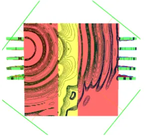
[image:7.595.225.373.533.671.2]Figure 5. Slices showing the norm of the real part of the total fieldE in the imaging chamber with the plastic-filled cylinder inside, for a transmitting antenna in the second ring from the top.
relative complex permittivity εgelr = 44 + 20i(see Figure 4). We consider the 32antennas of the
second ring from the top as transmitting antennas at frequency f = 1GHz, and all160 antennas are receiving. We evaluate the relative error on the reflection and transmission coefficientsSij with
respect to the coefficientsSref
ij computed from a reference solution. The relative error is calculated
with the following formula:
E=
q P
j,i|Sij−Sijref|2 q
P
j,i|Sijref|2
. (6)
The reference solution is computed on a fine mesh of approximately18million tetrahedra using edge finite elements of degreer= 2, resulting in114million unknowns. Slices in Figures4and5
show the computational domain and the solutionEfor one transmitting antenna in the second ring from the top.
We compare the computing time and the relative error (6) for different numbers of unknowns corresponding to several mesh sizes, for approximation degrees r= 1 and r= 2. All these simulations are done using512 subdomains with one MPI process and two OpenMP threads per subdomain, for a total of1024cores on the Curie supercomputer.
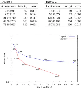
We report the results in TableIand in Figure6. As we can see, the high order approximation (r= 2) allows to attain a given accuracy with much fewer unknowns and much less computing time than the lowest order approximation (r= 1). For example, at a given accuracy ofE≈0.1, the finite element discretization of degreer= 1requires21million unknowns and a computing time of130
Table I. Total number of unknowns, time to solution (seconds) and relative error on the computedSij with respect to the reference solution for edge finite elements of degree1and2on different meshes.
Degree 1
# unknowns time (s) error
2 373 214 22 0.384
8 513 191 53 0.184
21 146 710 130 0.117
42 538 268 268 0.083
73 889 953 519 0.068
Degree 2
# unknowns time (s) error
1 508 916 39 0.243
5 181 678 62 0.099
12 693 924 122 0.057
26 896 130 236 0.036
45 781 986 396 0.019
0.01 0.1 1
0 50 100 150 200 250 300 350 400 450 500 550 2.4M
8.5M
21M
43M
74M 1.5M
5.2M
13M
27M
46M
relative error
time to solution (s)
Degree 1 Degree 2
Figure 6. Time to solution (seconds) and relative error on the computedSij with respect to the reference solution, using edge finite elements of degree1and degree2for different mesh sizes. The total number of
unknowns in millions is also reported for each simulation.
6. CONCLUSION
This work shows the benefits of using a discretization of the time-harmonic Maxwell’s equations based on high order edge finite elements coupled with a parallel domain decomposition preconditioner for the simulation of a microwave imaging system. In such complex systems, accuracy and computing speed are of paramount importance, especially for the application considered here of brain stroke monitoring.
Ongoing work consists in incorporating high order methods in the inversion tool that we are developing in the context of this application in brain imaging, for which promising results have already been obtained with edge finite elements of lowest order for the reconstruction from synthetic data of a numerical brain model.
We are also now in a position to test our inversion algorithm on various data sets acquired by the measurement system prototype of EMTensor.
iteration in the inversion loop corresponds to solving a linear system with multiple right-hand sides available simultaneously, with one right-hand side per transmitting antenna. Each direct problem with multiple right-hand sides can thus be solved efficiently by block methods such as Block GMRES, or by combining block and recycling strategies in a Block GCRO-DR algorithm. Block methods provide higher arithmetic intensity and better convergence.
Finally, choosing a suitable coarse space for the design of a scalable two-level preconditioner for Maxwell’s equations is still an open problem. Indeed, enriching the one-level preconditioner presented here with an efficient two-level preconditioner would lead to better convergence when using many subdomains, resulting in a highly scalable parallel solver.
REFERENCES
1. Semenov SY, Corfield DR. Microwave tomography for brain imaging: feasibility assessment for stroke detection. International Journal of Antennas and Propagation2008; .
2. Mikael P, Andreas F, et al. Microwave-based stroke diagnosis making global prehospital thrombolytic treatment possible.IEEE Transactions on Biomedical Engineering2014; .
3. Semenov S, Seiser B, Stoegmann E, Auff E. Electromagnetic tomography for brain imaging: from virtual to human brain.2014 IEEE Conference on Antenna Measurements & Applications (CAMA), 2014.
4. N´ed´elec JC. Mixed finite elements inR3.Numer. Math.1980;35(3):315–341, doi:10.1007/BF01396415. 5. Rapetti F. High order edge elements on simplicial meshes.M2AN Math. Model. Numer. Anal.2007;41(6):1001–
1020, doi:10.1051/m2an:2007049.
6. Rapetti F, Bossavit A. Whitney forms of higher degree. SIAM J. Numer. Anal. 2009;47(3):2369–2386, doi: 10.1137/070705489.
7. Bonazzoli M, Dolean V, Hecht F, Rapetti F. Overlapping Schwarz preconditioners for high order edge finite elements: application to the time-harmonic Maxwell’s equations 2016. Preprint HAL, https://hal.archives-ouvertes.fr/hal-01298938.
8. Bonazzoli M, Rapetti F. High order finite elements in numerical electromagnetism: degrees of freedom and generators in duality.Numerical Algorithms2015; Accepted with minor revisions.
9. Hecht F. New development in FreeFem++.J. Numer. Math.2012;20(3-4):251–265.
10. Dolean V, Jolivet P, Nataf F.An Introduction to Domain Decomposition Methods: algorithms, theory and parallel implementation. SIAM, 2015.
11. Cai XC, Sarkis M. A restricted additive Schwarz preconditioner for general sparse linear systems.SIAM J. Sci. Comput.1999;21(2):792–797 (electronic), doi:10.1137/S106482759732678X.
12. Dolean V, Gander MJ, Gerardo-Giorda L. Optimized Schwarz methods for Maxwell’s equations.SIAM J. Sci. Comput.2009;31(3):2193–2213, doi:10.1137/080728536.
13. Jolivet P, Hecht F, Nataf F, Prud’Homme C. Scalable domain decomposition preconditioners for heterogeneous elliptic problems.Proc. of the Int. Conference on High Performance Computing, Networking, Storage and Analysis, IEEE, 2013; 1–11.