On quantitative errors of two simplified unsteady models for simulating unidirectional nonlinear random waves on large scale in deep sea

City, University of London Institutional Repository

Citation

:

Wang, J., Ma, Q. & Yan, S. (2017). On quantitative errors of two simplified

unsteady models for simulating unidirectional nonlinear random waves on large scale in

deep sea. Physics of Fluids, 29(6), doi: 10.1063/1.4989417

This is the accepted version of the paper.

This version of the publication may differ from the final published

version.

Permanent repository link: http://openaccess.city.ac.uk/18492/

Link to published version

:

http://dx.doi.org/10.1063/1.4989417

Copyright and reuse:

City Research Online aims to make research

outputs of City, University of London available to a wider audience.

Copyright and Moral Rights remain with the author(s) and/or copyright

holders. URLs from City Research Online may be freely distributed and

linked to.

City Research Online:

http://openaccess.city.ac.uk/

[email protected]

1

On Quantitative Errors of Two Simplified Unsteady Models for

Simulating Unidirectional Nonlinear Random Waves on Large

Scale in Deep Sea

Jinghua Wang1_{, Q.W. Ma}1,a) _{and Shiqiang Yan}1

1_{School of Mathematics, Computer Science and Engineering, City, University of London, London, EC1V 0HB, UK}

To investigate nonlinear random wave dynamics or statistics, direct phase-resolved numerical simulation of nonlinear random waves in deep sea on large-spatial and long-temporal scales are often performed by using simplified numerical models, such as these based on the Nonlinear Schrödinger Equation (NLSE). They are efficient and can give sufficiently acceptable results in many cases but they are derived by assuming narrow bandwidth and small steepness. So far, there has been no formula to precisely predict the quantitative errors of such simplified models. This paper will present such formulas for estimating the errors of Enhanced NLSE based on Fourier transform and Quasi Spectral Boundary Integral (QSBI) method when they are applied to simulate ocean waves on large-spatial and long-temporal scales (about 128 peak wave lengths and 1000 peak periods). These formulas are derived by fitting the errors of the simplified models, which are estimated by comparing their wave elevations with these obtained by using a fully nonlinear model for simulating the cases with initial conditions defined by two commonly-used ocean wave spectra with a wide range of parameters. Based on them, the suitable regions for the simplified models to be used are shown.

1 INTRODUCTION

It is now increasingly recognized that direct and accurate simulation of ocean waves considering sufficient nonlinearity is necessary for understanding their dynamics. The simulation is challenging, not only due to the randomness and nonlinear effects of ocean waves, but also the fact that it needs to be carried out in a quite large scale and for a long duration1_.

To do that, phase-averaged models, such as WAM, WAVEWATCH and SWAN etc., are very popular2-4_{. The}

models are based on linear wave energy transportation equation with all nonlinear effects modelled by empirical source terms. They give the approximated evolution of wave spectra and wave statistical parameters such as significant wave height. A great success has been achieved using these models, so that we all benefit from the forecast of the wave statistics provided by, e.g, ECMWF, NOAA and Met Office UK. Nevertheless, in many applications and situations, one requires more specific and accurate information rather than just wave statistics such as direct velocity fields, acceleration fields and wave slopes of nonlinear ocean waves to gain better understanding of random waves dynamics. To achieve such goals, phase-resolved models should be employed1,5_.

In this class of models, the dynamic equations governing the velocity and wave elevation are directly solved in time domain and so such information becomes available throughout the space at all time steps. Among them, numerical models based on the Navier-Stokes (short as NS) equation or coupled potential & NS model6,7 _{may be}

employed but they are computationally prohibitive for large scale simulations. Nevertheless, the models based on nonlinear potential theory alone are much faster, and thus a brief review is given below.

One class of such models are fully nonlinear potential methods based on Finite Difference Method8-10_,

Boundary Element Method11,12_{, and Finite Element Method}13,14 _{or Quasi Arbitrary Lagrangian-Eulerian Finite}

Element Method15,16_{. However, they are still computationally expensive for very large scale simulations, thus}

barely applied so far to model waves in a scale of hundred wave lengths for thousand wave periods.

Another class of nonlinear models are these based on or associated with use of the Fast Fourier Transform (FFT), such as FFT mixed global minimizing approach17_{, FFT mixed lower-upper matrix decomposition method}18

and FFT mixed finite difference scheme19_{, Spectral Continuation method}20-22_{, Irrotational Green-Naghdi model}23_,

Higher-Order Spectral (HOS) method24,25_{, Spectral Boundary Integral method}26-28 _{and Enhanced Spectral}

Boundary Integral (ESBI) method29_{. This class of models is relatively faster but still needs significant amount of}

time. For an example, a 3D random sea simulation covering 42×42 peak wave lengths for 250 peak wave periods takes 10 CPU days on a 3 GHz-Xeon single processor PC by using the HOS method30_.

To be more efficient, researchers have developed many simplified potential models. One group of the models is the second order wave models, but Kriebel31,32 _{indicated that they could not describe the continuous spectral}

energy transfer between wave components as the amplitude of each wave component was independent of time, and thus they were only sufficiently accurate when the wave steepness was quite small (i.e., when the energy transfer between wave components was insignificant). The other group is the shallow water models, i.e., Boussinesq and KdV equations33,34_{, including the higher order versions}35-37_{. They are suitable for weakly nonlinear}

shallow water waves38,39_{, thus will not be further discussed as this paper focuses only on the waves in deep seas.}

Another class of simplified models for simulating waves in deep seas are these based on the Zakharov equation40-42 _{or nonlinear Schrödinger equation (shortened as NLSE)}40-44_{. The NLSE has a number of different}

versions, such as the cubic NLSE (shortened as CNLSE)40-44_{, the NLSE using the Dysthe equation}45,46_{, the}

Modified NLSE (shortened as MNLSE)47_{, the Enhanced NLSE (shortened as ENLSE-4 )}48_{, the Higher-Order}

Dysthe equation in terms of the Hilbert transform (shortened as ENLSE-5H)49_{, the Enhanced NLSE based on}

Fourier transform (shortened as ENLSE-5F)50 _{and the Hamiltonian higher-order NLSE}78-80_{. These methods are}

based on the assumption that the bandwidth of random waves is narrow. In addition, Wang, et al.50 _{suggested a}

simplified method called QSBI (Quasi Spectral Boundary Integral) method, which is obtained from simplifying the fully nonlinear ESBI method29 _{by only keeping the convolution terms up to the third order while ignoring the}

integration terms for evaluating the vertical velocity. This method can be applied to simulate random waves without limitation on bandwidth.

Applications of NLSE models to the direct simulation of random seas on large-spatial and long-temporal scales are extensive. For example, Onorato, et al.51 _{employed the CNLSE and performed more than 300}

simulations of random sea states on a scale of 100 peak wave lengths (L0) and 25 peak periods (T0), and found

that rogue waves are more likely to occur when the initial wave steepness is large. Dysthe, et al.52 _{studied the}

evolution of the wave spectra based on both the CNLSE and the ENLSE-4 in a domain covering 100L0×100L0

for 150T0, and found a power law behavior k−2.5 for integrated spectra53. Later, Dysthe, et al.54 and

Socquet-Juglard, et al.55 _{simulated 3D random seas covering 128L}

0×128 L0 for 150T0 based on the ENLSE-4, and pointed

out that the probability density of surface elevation fits the Tayfun distribution very well. In addition, Shemer, et al.56 _{studied the probability of rogue waves in a domain of 77 L}

0 for 100T0 based on both the CNLSE and the

Dysthe equation, and pointed out that the probability of rogue waves reaches the highest when the local bandwidth attains the maximum. Subsequently, Onorato, et al.57 _{brought the effects of current into the CNLSE and showed}

that rogue waves can be triggered naturally when a stable wave train enters a region of an opposing current flow field, based on a numerical simulation in a domain of 60 L0 for period of 60 T0. Later, Ruban58 considered the

L0 for 1000 T0. It is concluded that the reason of rogue wave occurrence is because of the interaction of

quasi-soliton coherent structures. Meanwhile, Zeng & Trulsen59 _{developed a NLSE for uneven bottom to simulate}

random waves propagating over 143L0 for 159 T0, and indicated that a change of water depth can provoke a

spatially non-uniform distribution of kurtosis on the lee side of the slope. More recently, Sergeeva, et al.60

simulated random waves in coastal regions on a scale of 20~40 L0 for up to 80 T0 based on a variable CNLSE,

and found that rogue waves are likely to occur at deeper locations. Taklo, et al.61 _{also simulated a random sea on}

a scale of 70L0 for 400T0 based on the Zakharov equation and found that the measured dispersion relation deviates

from the linear dispersion relation when the bandwidth is sufficiently narrow. Adcock, et al.62 _{recently applied the}

MNLSE to simulate random waves spanning 22L0×22 L0 for 300 T0 and suggested that the nonlinearity can give

a small amount of extra elevation above that of linear theory, but the nonlinear dynamics does change the shape and structure of extreme waves. Moreover, Simanesew, et al.63 _{used the MNLSE to simulate random waves}

covering 100L0×100 L0 for 200T0 and compared with laboratory results, then suggested that a strong

frequency-dependence of the directional spread will develop due to nonlinear effects. Zhang, et al.64 _{also employed the}

MNLSE to simulate random waves on the scale of 256L0×256L0 for 60 T0, and found that the statistical properties

of the simulated wave fields are basically consistent with the laboratory observation. Clamond, et al.65 _{carried out}

a long time simulation of soliton evolution by using the CNLSE, ENLSE-4 and their fully nonlinear method. They demonstrated that the ENLSE-4 model was more accurate than the CNLSE by showing that the results of the CNLSE started to become notably different from the results of their fully nonlinear method at 100 periods while these from ENLSE-4 were almost the same as those of the fully nonlinear method even at 150 periods. Wang66

confirmed the observation of Clamond, et al.65 _{and indicated that the results of the ENLSE-5F model is correlated}

well with the fully nonlinear results at 500 periods when the results of ENLSE-4 became quite different from the latter. The additional tests (not presented here) carried out by Wang66 _{also show that the MNLSE and ENLSE-4}

models give almost the same results and are more accurate than the CNLSE and other lower order NLSE models, but less accurate than the ENLSE-5F in long time simulations. The QSBI method has just been proposed and only applied as an alternative for the NLSE in the hybrid model of Wang, et al.50_{. That paper just demonstrates that the}

QSBI method is generally more accurate than the ENLSE-5F model but takes more computational time. Although these simplified models are computationally efficient, they are accurate in limited conditions. Dysthe, et al.52 _{had pointed out that for narrow bandwidth waves the CNLSE and MNLSE is reliable only when}

a dimensionless time scale (the time multiplied by peak circular frequency) is up to 2ε-2 _{and 10ε}-2 _{(ε peak wave}

number times amplitude), respectively. This information is very useful but it does not tell what is the specific values of errors if the models are employed. Xiao67 _{compared the results obtained by their HOS method and two}

NLS-type methods (MNLSE and NLSE using the Dysthe equation), and showed that the NLS-type methods could produce similar results to the HOS method when the spectrum change is slow, otherwise the results of NLS-type methods might be significantly different from those of the HOS method. It is desired that one would quantitatively estimate the errors of the simplified methods when applying them to simulate the random waves. According to the latest literature, the way to quantitatively and precisely estimate their errors seems not to be available, at least in public domain.

about the linear model is because it is often employed in practice and it would be useful to know its errors.

2 METHEDOLOGIES

In order to obtain the quantitative errors, the fully nonlinear method (ESBI) and the simplified models will be applied to simulate a large number of cases, whose initial conditions are defined by two different but commonly-used ocean wave spectra with a wide range of wave parameters. For each of the cases, the errors of the simplified models are estimated by comparing their wave elevations with these obtained by using the ESBI at the end of the simulation. After the errors of all cases are obtained, the formulas are formulated by using a data fitting technique.

All the numerical models have been documented in the publications cited above. Their formulations will only be briefed for completeness in the following sections. For convenience, all the variables involved will be non-dimensionalised in a consistent way, e.g., the length variables multiplied by peak wave number 𝑘0, and the

time variables multiplied by peak circular frequency 𝜔0, where

𝜔

= √𝑔𝑘

All the dimensionless variables are listed in Table I.

A. The ESBI and QSBI

The Spectral Boundary Integral (SBI) method has been suggested by Clamond & Grue26_{, Fructus et al.}68 _and

Grue28_{. It was improved and named as the ESBI by Wang & Ma}29 _{and Wang et al}50_{. This method is based on the}

potential theory with the boundary conditions on the free surface formulated as the skew-symmetric prognostic equation

𝜕𝑴

𝜕𝑇 + 𝚲𝑴 = 𝑵 (1)

where

𝑴 = ( 𝐾𝐹{𝜂}

𝐾Ω𝐹{𝜙̃}) , 𝚲 = [0 −ΩΩ 0 ] , 𝑵 = (

𝐾(𝐹{𝑉} − 𝐾𝐹{𝜙̃})

𝐾Ω𝐹 {1₂[(𝑉+∇𝜂∙∇𝜙_1+|∇𝜂|̃ )₂ 2− |∇𝜙̃|2]}) (2)

where 𝜂 and 𝜙̃ are the dimensionless free surface elevation and the velocity potential on the free surface, respectively, as shown in Table I that also includes the definition of other dimensionless variables; V is the dimensionless vertical velocity defined by 𝑉 = 𝜕𝜙/𝜕𝑛√1 + |∇𝜂|2_{, 𝛺 is the dimensionless frequency defined}

by 𝛺 = √𝐾 with 𝐾 = |(𝜅, 𝜁)| = √𝜅2_{+ 𝜁}2_{. In the above equations, the Fourier transform 𝐹{ } and the inverse}

transform 𝐹−1_{{ } are given by}

𝜂̂(𝑲, 𝑇) = 𝐹{𝜂} = ∫ 𝜂(𝑿, 𝑇)𝑒∞ −𝑖𝑲∙𝑿_𝑑𝑿

−∞ (3)

𝜂(𝑿, 𝑇) = 𝐹−1_{{𝜂̂} =} 1

4𝜋2∫ 𝜂̂(𝑲, 𝑇)𝑒𝑖𝑲∙𝑿𝑑𝑲 ∞

−∞ (4)

The solution for Eq.(1) is expressed by

𝑴(𝑇) = 𝑒−𝚲(𝑇−𝑇₀)_{∫ 𝑒}𝑇 𝚲(𝑇−𝑇₀)_𝑵𝑑𝑇

𝑇₀ + 𝑒

−𝚲(𝑇−𝑇₀)_𝑴(𝑇

0) (5)

𝑒𝚲∆𝑇_{= [cos Ω∆𝑇 − sin Ω∆𝑇}

sin Ω∆𝑇 cos Ω∆𝑇 ] (6)

The vertical velocity 𝑉 can be split into four parts, i.e., 𝑉 = 𝑉1+ 𝑉2+ 𝑉3+ 𝑉4 (see Eqs. (B.1)~(B.4) in

APPENDIX B). In the study of Wang & Ma29_{, several numerical techniques had been proposed in order to improve}

the computational efficiency. Firstly, they introduced a new numerical de-singularity technique to evaluate the integration parts more efficiently. Secondly, they reformulated the equations for 𝑉3 and 𝑉4 as (Eqs. (B.5)~(B.10)

in APPENDIX B)

𝑉3= 𝑉3,𝐶+ 𝑉3,𝐼= 𝑉⏟3(1) 4𝑡ℎ

+ 𝑉_⏟3(2)

6𝑡ℎ

+ 𝑉⏟3,𝐼

𝑖𝑛𝑡𝑒𝑔𝑟𝑎𝑡𝑖𝑜𝑛 (7)

𝑉4= 𝑉4,𝐶+ 𝑉4,𝐼 = 𝑉⏟4(1) 3𝑟𝑑

+ 𝑉⏟4(2) 5𝑡ℎ

+ 𝑉⏟4(3) 7𝑡ℎ

+ 𝑉⏟4,𝐼

𝑖𝑛𝑡𝑒𝑔𝑟𝑎𝑡𝑖𝑜𝑛 (8)

During the simulation, the wave properties are examined. The integration parts are evaluated only when their effects are significant; otherwise they are neglected. In such a way, computational time is saved without degrading the accuracy of numerical results. Thirdly, they developed a new technique for anti-aliasing to eliminate aliasing problems associated with convolutions in the above equations.

The QSBI (Quasi Spectral Boundary Integral) method is a simplified form of the ESBI method suggested by Wang, et al.50_{. In this method, the velocity accounts only for the convolution terms up to the third order and}

neglecting the integration terms, i.e., 𝑉 = 𝑉1+ 𝑉2+ 𝑉4(1) with others being the same.

The ESBI model had been validated in different situation as described in Wang and Ma29 _{and Wang, et al.}50_,

which showed the good accuracy of the method. One of the validated cases is summarized here. In this case, the ESBI is used for the simulation of a Stokes wave perturbed by a directional side-band wave 𝛿𝜂 = 0.025𝜖[𝑠𝑖𝑛(𝑲𝟏∙ 𝑿) + 𝑠𝑖𝑛(𝑲𝟐∙ 𝑿)] , where 𝜖 = 0.2985 , 𝑲𝟏= (3/2, 4/3) and 𝑲𝟐= (3/2, −4/3) . The

computational domain covers 2×1.5 Stokes wave lengths on transversal and longitudinal direction and is resolved by 28_{× 2}8 _{points. The duration of the simulation is 18 wave periods. For this case, Fructus, et al.}68

presented a quantitative result of the ratio

Ψ

= |𝐹{𝜂}|

/|𝐹{𝜂}|

|𝐹{𝜂}|

result is re-produced in FIG. 1. A code based on the method in Fructus, et al.68 _{was also programmed, which is}

referred to as the Fructus method and used to compute the same case. Both results are compared with that from the ESBI in FIG. 1. It shows that the code for the ESBI produces almost the same result as the Fructus method and the error at the end of the simulation is about 0.2%. The robustness and accuracy of the ESBI model has also been shown by other publications27,38,65_.

B. The ENLSE-5F

As indicated above, there are many different forms of NLSE models. For the purpose of this paper, the ENLSE-5F model will be used. That is because of the following considerations. Compared with other lower order counterparts based on the Dysthe equation, this one is the most accurate but does not require significantly more computational time. Compared with Hamiltonian higher-order NLSEs78-80_{, the ENLSE-5F model is chosen by}

to the wave elevation. This feature makes it relatively more difficult to transform between the free surface elevation and the wave action, in particular, from the wave elevation to the wave action. (ii) Detailed analysis (not presented in this paper) can show that the leading order of error of the ENLSE-5F is 𝜇3_𝜀3 _{while that of}

Hamiltonian higher-order NLSEs presented by both Craig, et al.79 _{and Gramstad & Trulsen}80 _{is 𝜇}2_𝜀3_{, where 𝜇}

and 𝜀 denote the magnitude of the bandwidth and the wave steepness, respectively. One of the purposes of this paper is to quantify the error of NLSE and the boundary of suitability. From their orders of error, it can be seen that the error of ENLSE-5F would not be larger than that of Hamiltonian higher-order NLSEs and so its boundary of suitability should cover the boundary of suitability of Hamiltonian higher-order NLSEs. In other words, in the region where ENLSE-5F is not valid or not sufficiently accurate, Hamiltonian higher-order NLSEs should not be sufficiently accurate either. (iii) Although the NLSE equations based on the Dysthe equation, including ENLSE-5F may not theoretically guarantee the conservation of the Hamiltonian (total wave energy) in finite and shallow waters, the effect of the problem is not significant in deep water concerned about in this paper, as indicated by Craig, et al.79_{. Socquet-Juglard, et al.}55 _{showed numerically that the MNLSE conserved the total energy to high}

accuracy within the bandwidth constraint for the cases they considered. Tests have been carried out on the Hamiltonian estimated by using the ENLSE-5F for a typical case with strong nonlinearity considered in this paper, and the results (not presented here) demonstrated that the error of the Hamiltonian is less than 0.2% for the simulation up to 1000 peak periods. However, for the cases in finite and shallow water, Hamiltonian higher-order NLSEs may be better, which will be studied in future work.

The ENLSE-5F model was suggested by Debsarma & Das49_{, and later modified by Wang, et al.}50_{. In the}

method, the free surface elevation and velocity potential are written in the summation of several harmonics by introducing the envelope45_{, i.e.,}

𝜂 = 𝜂̅ +1

2(𝐴𝑒𝑖𝜃+ 𝐴2𝑒2𝑖𝜃+ 𝐴3𝑒3𝑖𝜃+ 𝑐. 𝑐. ) (9)

𝜙 = 𝜙̅ +1

2[𝐵𝑒𝑖𝜃+𝑍+ 𝐵2𝑒2(𝑖𝜃+𝑍)+ 𝐵3𝑒3(𝑖𝜃+𝑍)+ 𝑐. 𝑐. ] (10)

where 𝐴 and 𝐵 are complex envelops of the first harmonic of free surface elevation and velocity potential respectively, 𝐴2, 𝐴3, 𝐵2 and 𝐵3 are the complex envelope coefficients of the high-order harmonics, 𝜂̅ and 𝜙̅

are slowly varying parts of free surface elevation and velocity potential45_{, 𝑐. 𝑐. represents the complex conjugate,}

and 𝜃 = 𝑋 − 𝑇. The envelop A satisfies the following equations

𝜕𝐴 𝜕𝑇+ 𝐹

−1_{{𝑖(𝜔 − 1)𝐹{𝐴}} = −}𝑖 2|𝐴|

2_{𝐴 −}3 2|𝐴|

2 𝜕𝐴 𝜕𝑋−

1 4𝐴

2 𝜕𝐴∗ 𝜕𝑋 +

𝑖 2𝐴𝐹

−1_{{|𝜅|𝐹{|𝐴|}2_{}} +}

5𝑖 8|𝐴|

2 𝜕2𝐴 𝜕𝑋2+

9𝑖 16𝐴

∗₍𝜕𝐴 𝜕𝑋)

2

+₈𝑖𝐴_𝜕𝑋𝜕𝐴𝜕𝐴_𝜕𝑋∗−₈𝑖𝐴2 𝜕2𝐴∗ 𝜕𝑋2 +

1 2

𝜕𝐴 𝜕𝑋𝐹

−1_{{|𝜅|𝐹{|𝐴|}2_{}} +}

1 4𝐴𝐹

−1_{{|𝜅|𝐹 {𝐴}𝜕𝐴∗ 𝜕𝑋}} +

1 2𝐴𝐹

−1_{{|𝜅|𝐹 {𝐴}∗ 𝜕𝐴 𝜕𝑋}} +

𝑖 8𝐴𝐹

−1_{𝜅2_𝐹{|𝐴|2_}}

(11)

The other parameters (𝐴2, 𝐴3, 𝐵2, 𝐵3 𝜂̅ and 𝜙̅) are estimated by using Eqs. (A.1)~(A.6) in APPENDIX A. The

numerical code for the ENLSE-5F model has been validated in Wang, et al.50 _{and Wang}66_{, which will not be}

repeated here.

3 NUMERICAL SIMULATIONS AND RESULTS

which the linear model is simply described by Eq. (14) below.

All the models will be applied to simulate the defined cases with different parameters. The simulations start by specifying the initial values on the free surface, which are determined by using widely-used JONSWAP and Wallops spectra. The JONSWAP is often employed to represent developing sea states69_{, which is given in terms}

of non-dimensional parameters in Table I by

𝑆𝐽(𝑘) =

𝛼𝐽𝐻𝑠2

2𝑘3 exp [−

5 4(

1 𝑘)

2

] γexp[−(√𝑘−1)2/(2σ2) ] (12)

where 𝐻𝑠 is the non-dimensional significant wave height (multiplied by peak wave number), 𝛼𝐽=

0.0624(1.094 − 0.01915lnγ)/(0.23 + 0.0336γ − 0.185(1.9 + γ)−1_{), γ is the peak enhancement factor, and}

𝜎 = 0.07 for 𝑘 < 1 or 0.09 for 𝑘 ≥ 1. The bandwidth becomes narrower when γ increases. To represent developed sea states, the Wallops spectrum is often adopted as suggested by Goda69_{, which can be expressed by}

𝑆𝑊(𝑘) =

𝛽𝐻𝑠2

2𝑘(𝑚+1)/2𝑒𝑥𝑝 [−

𝑚

4𝑘2] (13)

where 𝛽 = 0.06238𝑚(𝑚−1)/4_/(4(𝑚−5)/4_{Γ[(𝑚 − 1)/4])[1 + 0.7458(𝑚 + 2)}−1.057_{] and 𝑚 controls the}

bandwidth with the spectrum becoming narrower as 𝑚 increases.

Corresponding to the spectra, the initial linear free surface elevation in the whole domain may be written as

𝜂′(𝑋, 𝑇 = 0) = ∑ 𝑎𝑗𝑐𝑜𝑠(𝑘𝑗𝑋 − 𝜔𝑗𝑇 + 𝜑𝑗)_𝑇=0 𝑁𝐽

𝑗=1

= ∑ 𝑎𝑗𝑐𝑜𝑠(𝑘𝑗𝑋 + 𝜑𝑗) 𝑁𝐽

𝑗=1

(14)

where 𝑎𝑗= √2𝑆(𝑘𝑗)Δ𝑘, 𝑆(𝑘) can be 𝑆𝐽(𝑘) or 𝑆𝑊(𝑘), and 𝜑𝑗 is randomly distributed in [0,2𝜋), 𝑘𝑗 is the

wave number of the 𝑗𝑡ℎ component, 𝜔𝑗= √𝑘𝑗, 𝑁𝐽 is the total number of the components. The limitation by

using Eq.(14) (i.e., the random phase technique) was discussed in Tucker, et al.70_{, who suggested to use the random}

amplitude approach to give the initial free surface elevation. However, according to Elgar, et al.71_{, for a sufficiently}

large number of spectral components (1000 or more), no significant differences were found in the statistics produced by the two techniques. According to this, the total number of components considered is 1024 in the study. More discussions about this will be presented in Section 4.

It is noted that 𝜂′ by Eq. (14) is merely the free modes. The initial free surface elevation with the bound modes can be constructed by using the technique summarised in APPENDIX C, which was introduced in Wang, et al.50_{. The initial free surface conditions may be specified by either considering only the free modes (Eq. 14) or}

the free modes plus the bound modes. As one of the purposes of this study is to quantify the error of the 5F, the simulation of all methods should start with the same initial conditions normally employed by the ENLSE-5F, consisting both free modes and bound modes. In such a way, the errors between their results are mainly attributed to the method itself. If the initial conditions would not be the same, the errors should have included the effects of initial condition, which should not be considered for assessing the accuracy of the methods. Based on these considerations, all simulations for obtaining the results discussed hereafter are carried out by using the initial free surface elevation consisting of both free and bound modes.

A. Computational parameters

To perform the numerical studies, the computational parameters need to be properly selected. This section will discuss how to choose the proper parameters.

the Wallops spectrum, respectively. In order to quantify the errors of the simplified models, the range of the parameters must be large enough. According to Goda69_{, the practical range of γ is within [1, 9] while it is within}

[5, 25] for m, which will be used in the study here. In the later sections, the central moment72 _{defined by}

𝑚𝑐= ∫ |𝑘 − 1|

𝑆(𝑘) 𝐻𝑠2 𝑑𝑘 +∞

0

(15)

will be used. The relationship between 𝑚𝑐 and the bandwidth parameters can be established through curve fitting

and is given directly here without further details for simplicity, i.e.,

𝑚𝑐 = 0.181 exp(−0.917𝛾0.300) (16)

for the JONSWAP spectrum, while

𝑚𝑐= 0.005 exp(7.807𝑚−0.674) (17)

for the Wallops spectrum. The fitted results by the two equations are shown in FIG. 2, where the values denoted by ‘target’ are those calculated directly by Eq.(15). The maximum error between the target (Eq.15) and fitted results (Eq.16 or Eq.17) are 0.3% and 2.0%, respectively, which is invisible in the figure. From this figure, one can see that the range of 𝑚𝑐 is 0.031 ≤ 𝑚𝑐≤ 0.072 for the JONSWAP spectrum and 0.012 ≤ 𝑚𝑐 ≤ 0.072

for the Wallops spectrum with respect to the chosen range of 𝛾 and 𝑚.

The non-dimensional significant wave height (𝐻𝑠) actually represents the wave steepness or nonlinearity of

the initial free surface elevation as defined in Table I. Note that there are several ways to represent the random wave steepness (𝜀), e.g., Dysthe, et al.54 _{used 𝜀 = √2𝜎, where 𝜎}2_{= ∫ 𝑆(𝑘)𝑑𝑘}

_{. As}

𝑠= 4𝜎, one obatins 𝐻𝑠=

2√2𝜀, which means 𝐻𝑠 is directly related to the steepness of the random waves. If it is very small, the waves can

be well described by the linear model. Based on this, the lower end of the range of 𝐻𝑠 (i.e. its smallest value for

the numerical study) is taken as 0.001. The results given in later sections will show that in the ranges of γ and m chosen above, the linear model can very well predict the evolution of waves when 𝐻𝑠≤ 0.001 (equivalently,

𝜀 ≤ 0.0004).

The question is that what is the largest value of 𝐻𝑠 (i.e., the upper end of its range) to be chosen for the

numerical studies. It is well known that with the increase of the steepness, the nonlinearity of the waves becomes stronger, the accuracy of the three simplified models decreases and so their errors increase. A model should be considered as unsuitable if its error is larger than a certain value, defined as ERup. In this paper, ERup is chosen to

be 20%. The upper end of 𝐻𝑠 should be chosen to be the value, corresponding to which the error of all three

simplified models is smaller than ERup. According to our numerical tests discussed in later sections, the upper end

of 𝐻𝑠 can be taken as 0.18 (𝜀 ≈ 0.064). Based on the above discussions, the range and specific values of each

parameter chosen for numerical studies here are summarised in Table III.

For the numerical studies, the computational domain is set as 128 peak wave lengths, which is more than 20 km if the peak wave period is 10 seconds or more. Based on the tests presented in Wang et al.50 _{and Wang & Ma}29_,

the domain is resolved into 8192 points for all the models in Table II. To show the resolution is sufficient, the cases with 𝐻𝑠 = 0.15 & 𝑚 = 5 for the Wallops spectrum and 𝐻𝑠 = 0.15 & γ = 1 for the JONSWAP

B. Effects of duration of simulations

In this subsection, the effects of the duration of simulations will be investigated. The duration should be long enough so that the random waves are fully developed. To quantitatively measure the degree of the wave development, the abnormality indexes72 _{are introduced, i.e.,}

𝐴𝐼𝐺(𝑇) =

|𝜕𝜂/𝜕𝑋|𝑚𝑎𝑥

|𝜕𝜂/𝜕𝑋|𝑠 , 𝐴𝐼𝐻(𝑇) =

𝐻𝑚𝑎𝑥

𝐻𝑠 (18)

where 𝐴𝐼𝐺 and 𝐴𝐼𝐻 are both functions of 𝑇, subscript ‘max’ represents the maximum value detected within the

time range [0, 𝑇], |𝜕𝜂/𝜕𝑋|𝑠 is the significant gradient computed by using the initial free surface profile. The

two indexes are closely related to the wave statistics and dynamics. For example, 𝐴𝐼𝐻 is used for measuring the

maximum waves height, which is traditionally adopted for examining the survivability of structures73_{. While 𝐴𝐼}

𝐺

describes the maximum slope of the free surface, on which the wave impact force depends74_.

In order to illustrate how the two indexes evolve with time, the cases with 𝐻𝑠= 0.15 & 𝑚 = 5 for the

Wallops spectrum and 𝐻𝑠= 0.15 & γ = 1 for the JONSWAP spectrum (𝜀 ≈ 0.053) are simulated. The time

histories of 𝐴𝐼𝐺 and 𝐴𝐼𝐻 corresponding to the cases are plotted in FIG. 3. From the figures, one can see that

𝐴𝐼𝐺 is not stabilized until 𝑇/𝑇0= 300 while 𝐴𝐼𝐻 becomes stable only after 𝑇/𝑇0= 600. Based on this and

other tests we carried out, the duration of simulation can be taken as 1000𝑇0 to ensure the waves are fully

developed. The duration is about 3 hours in real time if the peak period is more than 10 seconds.

FIG. 3 also shows that 𝐴𝐼𝐺 and 𝐴𝐼𝐻 at the end of simulations obtained by using the ESBI are much higher

than these of initial values specified and obtained by using the linear model. In addition, FIG. 3(a) and (c) show that the 𝐴𝐼𝐺 obtained by using ESBI is almost double of the initial values and that obtained by using the linear

model, while the 𝐴𝐼𝐻 from the ESBI is more than 1.5 times larger than others. Compared with the initially

specified steepness (i.e., 0.15 in the cases), the obtained maximum slope of the free surface is 0.816 (i.e., 6.8×0.15).

C. Effects of random phases

As discussed above, the initial free surface elevation depends on Eq.(14), which is not deterministic but random as the phase 𝜑𝑗 is random. The question that how this affects the error of each simplified model should

be answered priori to further explore the effects of different values of spectrum parameters. Thus some numerical tests are carried out in order to answer this question and the error of each simplified model is measured by

𝐸𝑟𝑟1,2,3=

∫ |𝜂₀𝐿𝑑 1,2,3− 𝜂0|𝑑𝑋

∫ |𝜂₀𝐿𝑑 0|𝑑𝑋

(19)

where 𝐸𝑟𝑟1~3 denote the error of the linear model, ENLSE-5F and QSBI, respectively; 𝜂1~3 is the

corresponding free surface spatial distribution obtained by the three models at the end of the simulation, 𝜂0 that

of the ESBI, and 𝐿𝑑 is the length of the computational domain. We will mainly focus on two matters: a) one is

about the trend of 𝐸𝑟𝑟1,2,3 evolving with time, and b) the other is the statistics of 𝐸𝑟𝑟1,2,3 at the end of the

simulation, e.g., average and standard deviation of the error, corresponding to different series of random phases. For this purpose, the cases with given 𝐻𝑠 and 𝛾 or 𝑚 are simulated using all the methods in Table II

starting with the same initial condition. The simulations for each set of the computational parameters are repeated 10 times but using a different series of random phases 𝜑𝑗. 𝐸𝑟𝑟1,2,3 are calculated for each time steps during the

simulations. Some examples of 𝐸𝑟𝑟1,2,3 varying with time are shown in FIG. 4, where lines with different colors

denote results correspond to different series of random phases. It can be seen that the values of 𝐸𝑟𝑟1,2,3

corresponding to the same parameters of 𝐻𝑠 and 𝛾 or 𝑚 are only slightly different for different series of

phases, the evolution of 𝐸𝑟𝑟1,2,3 does not behave significantly differently.

To further show the effects of random phases on 𝐸𝑟𝑟1,2,3 , the values of 𝐸𝑟𝑟1,2,3 for several sets of

computational parameters obtained at the end of the simulation are extracted. Their average and standard deviation are calculated and presented in Table IV and Table V for the JONSWAP and Wallops spectra, respectively. As can be seen, in the cases where the average error is less than 20%, the maximum standard deviation of the errors is only 1.7%. These data again demonstrate that the values of 𝐸𝑟𝑟1,2,3 are not sensitive to the choice of random

series of 𝜑𝑗.

D. Errors of different simplified models

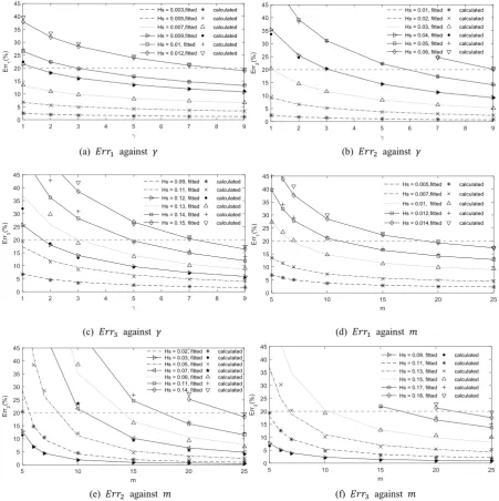
The errors of different simplified models are now presented and discussed. The method to evaluate the errors has been described above (Eq. (19)), i.e., they are computed by using the wave profiles after simulating the cases with different parameters given in Table III over the duration of 1000T0 by 4 different models (the linear model,

ENLSE-5F, QSBI and ESBI). For each case, all the four models start with the same initial free surface elevation determined by the method in Appendix C. The errors of the three simplified models (the linear model, ENLSE-5F and QSBI) are then calculated by applying Eq.(19) to the relevant free surface elevations obtained at the end of simulations. The obtained numerical errors in such way are shown by different symbols and indicated by ‘calculated’ in FIG. 5. It may be noted that the case with the maximum value of Hs is different in different figures.

That is because the cases with all the errors are larger than 20% are not plotted in the figures. For an example, in FIG. 5a, the error of the linear model is larger than 20% for the whole range of 𝛾 for any value of Hs>0.012 (𝜀 >

0.004) and so the results for the cases with Hs>0.012 are not plotted in the figure. Similarly, the errors for all the

other cases with the parameters given in Table III but not plotted in FIG. 5 are all larger than 20%. It may also be noted that the largest values of Hs in all the figures is 0.18, which indicates that all the simplified models have an

error larger than 20% if Hs>0.18 (𝜀 > 0.064). This also justifies why we only selected the cases with Hs ≤0.18

(corresponding to ERup= 20%) in Table III. As can be seen from these figures, the errors of each model generally

increase with the decrease of 𝛾 (or 𝑚) and the increase of 𝐻𝑠. With reference to Eq.(16) and (17), it may also

be said that the errors increase with the increase of 𝑚𝑐 and 𝐻𝑠. In addition, for all the values of 𝛾 and 𝑚, the

errors of the linear model obtained by using the JONSWAP and Wallops spectra are very small, less than 1% for 𝐻𝑠= 0.001 (𝜀 ≈ 0.0004), which means that the linear model is sufficiently accurate for simulating the cases if

the initial significant wave height is less than 0.001.

To mathematically represent the calculated errors in FIG. 5, it is assumed that the calculated errors of the three simplified models can be fitted by

𝐸𝑟𝑟1′= 𝑎1𝐻𝑠𝑏1𝑚𝑐𝑐1 (20)

𝐸𝑟𝑟2′= 𝑎2𝐻𝑠𝑏2𝑚𝑐𝑐2 (21)

𝐸𝑟𝑟3′= 𝑎3𝐻𝑠𝑏3𝑚𝑐𝑐3 (22)

where 𝑎𝑖 , 𝑏𝑖 and 𝑐𝑖 (i = 1, 2 or 3, corresponding to the linear model, ENLSE-5F and QSBI models) are

constants to be determined. These constants are determined by optimizing the following target function

𝕐𝑖(𝑎𝑖, 𝑏𝑖 , 𝑐𝑖) = ∑ (𝐸𝑟𝑟𝑖− 𝐸𝑟𝑟′𝑖)𝐽2

𝐽 (23)

where i is taken as 1, 2 or 3, corresponding to the linear model, ENLSE-5F and QSBI; 𝐸𝑟𝑟𝑖 are these given in

FIG. 5 by different symbols, i.e., the calculated values. Since the error larger than 20% may just indicate that a simplified model is not suitable for simulating the random waves as indicated before, only the data corresponding to 𝐸𝑟𝑟𝑖≤ 20% are considered for fitting the numerical results using Eqs.(20), (21) or (22). In order words, the

The optimization is performed by using the toolbox (Optimization-fminsearch) in MATLAB. The details of this toolbox can be found in MATLAB user manual which will not be provided here. After the optimizations are performed, the constants in the fitting formulae corresponding to the JONSWAP spectrum are given by

{

𝑎1= 1.922×104, 𝑏1= 1.967, 𝑐1= 0.811

𝑎2= 1.207×104, 𝑏2= 1.944, 𝑐2= 1.588

𝑎3= 3.847×105, 𝑏3= 4.564, 𝑐3= 1.726

(24)

and these corresponding to the Wallops spectrum are given by

{

𝑎1= 1.280×104, 𝑏1= 1.971, 𝑐1= 0.633

𝑎2= 4.593×104, 𝑏2= 1.961, 𝑐2= 1.942

𝑎3= 5.256×104, 𝑏3= 4.274, 𝑐3= 1.196

(25)

Now, replacing 𝑚𝑐 in Eqs. (20) ~ (22) with Eqs. (16) and (17), and substituting 𝑎1~3, 𝑏1~3 and 𝑐1~3 with

these in Eqs. (24) and (25), one has

𝐸𝑟𝑟1′= 4.805×103𝐻𝑠1.967exp(−0.744𝛾0.300) (26)

𝐸𝑟𝑟2′= 7.997×102𝐻𝑠1.944exp(−1.456𝛾0.300) (27)

𝐸𝑟𝑟3′= 2.013×104𝐻𝑠4.564exp(−1.583𝛾0.300) (28)

for the JONSWAP spectrum, while

𝐸𝑟𝑟1′= 447.4𝐻𝑠1.971exp(4.942𝑚−0.674) (29)

𝐸𝑟𝑟2′= 1.561𝐻𝑠1.961exp(15.161𝑚−0.674) (30)

𝐸𝑟𝑟3′= 93.03𝐻𝑠4.274exp(9.337𝑚−0.674) (31)

for the Wallops spectrum. The curves of 𝐸𝑟𝑟′

𝑖 are plotted in FIG. 5, denoted by ‘fitted’. One can see that there is excellent consistency

between the calculated and fitted results for all the cases with 𝐸𝑟𝑟1~3≤ 20%. The maximum differences between

the calculated and fitted results obtained by using the JONSWAP spectrum and Wallops spectrum are only 2.1% occurring at the point for 𝐻𝑠= 0.11 (𝜀 ≈ 0.039) and 𝛾 = 1 in FIG. 5c and 1.9% occurring at the point for

𝐻𝑠= 0.15 (𝜀 ≈ 0.053) and 𝑚 = 25 in FIG. 5f, respectively.

It is noted that as Eqs. (26)~(31) are obtained by using the cases with the parameters listed in Table III, they may be perceived to be only applicable within the range 0.001 ≤ 𝐻𝑠≤ 0.18 (0.0004 ≤ 𝜀 ≤ 0.064), 5 ≤ 𝑚 ≤

25 for Wallops spectrum and 1 ≤ 𝛾 ≤ 9 for JONSWAP spectrum. However, as aforementioned, the linear model can provide accurate results while 𝐻𝑠< 0.001 and the errors are larger than 20% if 𝐻𝑠> 0.18 . In

addition, when 𝐸𝑟𝑟1~3> 20%, it just indicates that the corresponding model cannot give acceptable results for

modelling the random sea in deep water. Taking all the facts into account, one may know from the results presented in this section that (1) when 𝐻𝑠< 0.001, the linear model can be used without significant error; (2) when 𝐻𝑠>

0.18, none of the three simplified models should be employed; (3) when 0.001 ≤ 𝐻𝑠 ≤ 0.18, one can estimate

the errors of the three simplified models: if the error of a model is less than 20%, this error needs to be accepted if using this model; if the error is larger than 20%, this model may not be employed.

𝐻𝑠1= 0.013 exp(0.378𝛾0.3) 𝑇𝑜𝑙0.508 (32)

𝐻𝑠2= 0.032 exp(0.749𝛾0.3) 𝑇𝑜𝑙0.514 (33)

𝐻𝑠3= 0.114 exp(0.347𝛾0.3) 𝑇𝑜𝑙0.219 (34)

and for the Wallops spectrum

𝐻𝑠1= 0.045 exp(−2.507𝑚−0.674) 𝑇𝑜𝑙0.507 (35)

𝐻𝑠2= 0.797 exp(−7.731𝑚−0.674) 𝑇𝑜𝑙0.510 (36)

𝐻𝑠3= 0.346 exp(−2.185𝑚−0.674) 𝑇𝑜𝑙0.234 (37)

where 𝐻𝑠𝑖 (i=1,2 or 3) is the maximum significant wave height for the linear model, ENLSE-5F and QSBI to be

employed, respectively.

More discussions about how to use Eqs. (26)~(31) and Eqs. (32)~(37) will be given in the following sections.

4 DISCUSSIONS

This section will discuss several points relevant to Eqs. (26)~(31) and Eqs. (32)~(37), including their possible applications to evaluating the simplified models that are employed to study the random wave dynamics or statistics.

A. Comparisons with the criterion of Dysthe, et al.’s52

Dysthe, et al.52 _{had pointed out that the CNLSE and MNLSE can be reliably used on a temporal scale up to}

2𝜀−2 _{and 10𝜀}−2 _{, respectively, for simulating narrow bandwidth waves (initial conditions determined by the}

Gaussian Spectrum). Based on them, for simulations of 1000 peak periods (𝑇0= 2𝜋), the CNLSE and MNLSE

can be used with the significant wave height (𝐻𝑠 = 2√2𝜀) up to about 0.05 and 0.11 (𝜀 ≈ 0.018 and 0.039),

respectively. The criterion of Dysthe, et al.52 _{is compared with these we suggested, i.e., Eqs. (32)~(37) for 𝑇𝑜𝑙 =}

10% in FIG. 8. The grey thicker dashed line denotes the up-limit of the MNLSE and the grey thinner dashed line represents that of the CNLSE based on the suitable temporal scale given by Dysthe, et al.52_{. It can be observed in}

both FIG. 8(a) and (b) that the up-limit of the MNLSE is significantly higher than these given for the ENLSE-5F model in this study, in particular for the cases corresponding to the JONSWAP spectrum. The former is only close to the latter when the Wallops spectrum with very narrow bandwidth (m>20) is used. It means that if the suggestion of Dysthe, et al.52 _{for MNLSE is followed, the results may have the error much larger than 10%. The same}

argument applies to the CNLSE employed for the JONSWAP spectrum as shown in FIG. 8(a). Furthermore, if the initial conditions of the CNLSE are specified by the Wallops spectrum, the up-limit of CNLSE model indicated by 2𝜀−2 _{is much different from what we give here even for the waves with a very narrow bandwidth. This implies}

that if the suggestion of Dysthe, et al.52 _{is followed, one would not obtain the results that bear the error of less}

than 10%.

B. Error prediction

Eqs. (26)~(31) can be employed for predicting the error of the simplified models. To illustrate their effectiveness, extra numerical tests are carried out for the cases with parameters listed in Table VI and Table VII, which are in the range of the parameters in Table III but different from those used for obtaining the results in FIG. 5. In the tables, the values of 𝐸𝑟𝑟1~3 are obtained in the same way as for FIG. 5, while the values of 𝐸𝑟𝑟1~3′ are

predicted by Eqs. (26)~(31) for the corresponding parameters. These errors represented by ‘-’ in the tables means that their values are larger than 20%. It is found that although the choices of the parameters differ from these in FIG. 5, Eqs. (26)~(31) can still satisfactorily give quite accurate prediction of the errors as long as 𝐸𝑟𝑟1~3< 20%.

To show the level of correlation between the error given in Eqs. (26)~(31) and wave elevations, some wave profiles at the end of the simulation corresponding to different level of errors are displayed in FIG. 6. It can be seen that as long as the predicted error is small, the differences between the elevations calculated by the simplified models and these by the ESBI are almost invisible. We have also examined the corresponding velocity and velocity potential, and found that the errors of the velocity and velocity potential are in the same magnitude as those of the wave elevations if 𝐸𝑟𝑟1~3< 20% (results are not presented here for shortening the length of the paper).

As aforementioned, some studies employ the random amplitude approach to convert the spectrum to the free surface elevation70,75_{. As discussed in the former section, the results of the random amplitude approach are}

approximately the same with these of the random phase approach when the number of wave component is large71_.

To show that Eqs. (26)~(31) are also correlated with the error in the cases where the random amplitude technique is adopted for generating the initial free surface condition, we carry out the numerical tests on the cases with the parameters in Table VI and Table VII by using the random amplitude approach. The calculated and predicted errors are shown in Table VIII and Table IX. It is found the maximum difference between the calculated errors obtained by using the random amplitude approach and these predicted by Eqs. (26)~(31) is only 1.6%. The spatial distribution of the free surface for some cases are also presented in FIG. 7. These figures show that the results are very similar to FIG. 6. All the facts demonstrate that Eqs. (26)~(31) can be used to predict the errors in the cases where random amplitude approach would be used for generating the initial free surface condition.

C. Suitability of simplified models

In order to study random waves on large-spatial and long-temporal scale in deep water efficiently and accurately, one should firstly determine suitable model among the linear model, ENLSE-5F, QSBI and ESBI. In this section, graphs showing the regions suitable for different models will be presented, which may help researchers to select a model.

When selecting the model, the acceptable error should be specified, such as no more than 5% as indicated by Wang, et al.50_{. Based on Eqs. (32)~(37), the graphs of the maximum significant wave height 𝐻𝑠}

𝑖 (i=1,2 or 3)

suitable for different models are plotted in FIG. 9 with respect to tolerant error 𝑇𝑜𝑙 = 5%. The graphs illustrate the regions in which different models are suitable. For example, the ENLSE-5F is suitable for simulating all the cases underneath the dot-dashed lines. It is illustrated that the maximum significant wave height for a specific model to be applied increases when the bandwidth becomes smaller (𝛾 or 𝑚 becomes larger) for both the spectra. The reason is that the terms ignored in the simplified model involves the bandwidth parameter. Such terms become more and more important and dominating when bandwidth increases, so that they become less accurate. As a consequence, in order to maintain the same level of accuracy, the maximum significant wave height that the simplified model could be applied becomes smaller as the bandwidth increases, or becomes larger as the bandwidth decreases (𝛾 or 𝑚 increases).

According to these aforementioned, it is suggested that the following conditions

𝐻𝑠≤ 𝐻𝑠1: Linear model (38)

𝐻𝑠1< 𝐻𝑠≤ 𝐻𝑠2: ENLSE-5F (39)

𝐻𝑠2< 𝐻𝑠≤ 𝐻𝑠3: QSBI (40)

𝐻𝑠> 𝐻𝑠3: Fully nonlinear model (41)

It is noted that for the very strong nonlinear cases the breaking wave will occur and so fully nonlinear model ESBI will not be suitable. The up-limit of the fully nonlinear model, beyond which breaking wave occurs, were discussed by Melville76 _{and Ochi & Tsai}77 _{for uniform wave cases. Identifying the up-limit of the ESBI is beyond}

the scope of this study, as we mainly focus on identifying the boundaries of the simplified models.

5 CONCLUDING REMARKS

This paper has presented the formulas for quantitatively estimating the errors of the Enhanced Nonlinear Schrödinger Equation based on Fourier transform (ENLSE-5F) and Quasi Spectral Boundary Integral (QSBI) method when they are applied for simulating nonlinear random waves in deep sea on large-spatial and long-temporal scales in a phase-resolved manner. The two groups of formulas are given, one for the initial conditions specified by the JONSWAP spectrum and the other by the Wallops spectrum. The suggested formulas can give good predictions on the errors of the simplified models as long as the errors are less than 20% within the range of bandwidth in 1 ≤ 𝛾 ≤ 9 or 5 ≤ 𝑚 ≤ 25 and the significant wave height in 𝐻𝑠 ≤ 0.18 (𝜀 ≤ 0.064 ). The ranges of bandwidth parameters are considered to cover the most cases met in real sea states according to the literature available. If the error is larger than 20% estimated by the formulas and/or 𝐻𝑠 > 0.18 (𝜀 > 0.064), it just means that the simplified models may not give acceptable results and so may not be employed. Although the formulas are obtained by using initial condition based on random phase approach, they also work for those cases based on random amplitude approach according to the numerical tests.

Based on the formulas, the suitable regions for the simplified models are plotted in terms of bandwidth parameters (𝛾 for the JONSWAP spectrum and m for the Wallops spectrum) and significant wave heights (i.e., peak wave number times significant wave height). The dimensionless maximum significant wave height up to which the simplified model could be applied becomes smaller as the bandwidth increases, or becomes larger as bandwidth decreases (𝛾 or 𝑚 increases), which are quite different from the qualitative indication available in literature.

This paper provides useful information for evaluating the simplified wave models that are employed for studying random wave dynamics, e.g., how reliable are the results obtained after using the simplified models, or which model should be selected in order to obtain acceptable results before carrying out the simulations. However, it should be pointed out that although the formulas proposed in this paper are based on the cases of unidirectional waves, they also give an indication of the errors for the simplified models to be applied for simulating spreading seas. However, further studies on their errors in simulating spreading seas will be carried out in the future.

ACKNOWLEDGMENTS

This work was supported by the EPSRC, UK (EP/N008863/1, EP/L01467X/1 and EP/N006569/1).

APPENDIX A: HARMONIC COEFFICIENTS

In order to estimate the free surface and velocity potential, each harmonic coefficient is given in terms of A by Wang, et al.50_{, which follow as}

𝐴2=

1 2𝐴2−

𝑖 2𝐴

𝜕𝐴 𝜕𝑋+

3 8𝐴

𝜕2_𝐴

𝜕𝑋2

(A. 1)

𝐴3=

3

𝐵 = 𝐹−1_{−𝑖

𝜔 𝐹 {𝐴 + 3

8|𝐴|2𝐴}} (A. 3)

𝐵2= 𝐵3= 0 (A. 4)

𝜙̅ = 𝐹−1_{{𝑠𝑔𝑛(𝜅)}𝑖

2𝐹{|𝐴|2}} (A. 5)

𝜂̅ = 𝐹−1_{{−𝑖𝑠𝑔𝑛(𝜅)𝐹{𝑟𝑒𝑎𝑙(𝐴}∗_𝐴

𝑇)}} −₁₆1 𝜕 2_|𝐴|2

𝜕𝑋2 (A. 6)

APPENDIX B: FORMULATIONS FOR VERTICAL VELOCITY

The formulations for estimating the convolution and integration parts in the vertical velocity V have been proposed by Grue28 _{and Wang & Ma}29_{, which are also presented below}

𝑉1= 𝐹−1{𝐾𝐹{𝜙̃}} (B. 1)

𝑉2= −𝐹−1{𝐾𝐹{𝜂𝑉1}} − ∇ ∙ (𝜂∇𝜙̃) (B. 2)

𝑉3= 𝐹−1{_2𝜋𝐾𝐹 {∫ 𝜙̃′[1 −_(1+𝐷12₎3/2]

(𝜂′−𝜂)−𝑹∙∇′𝜂′ 𝑅3 𝑑𝑿′

𝑆0 }} (B. 3)

𝑉4= −

𝐾

2[𝐾𝐹{𝜂2𝑉} − 2𝐹 {𝜂𝐹−1{𝐾𝐹{𝜂𝑉}}} + 𝐹 {𝜂2𝐹−1{𝐾𝐹{𝑉}}}]

+ 𝐾 2𝜋𝐹 {∫

𝑉′

𝑅(1 − 1 √1 + 𝐷2−

1

2𝐷2) 𝑑𝑿′}

(B. 4)

𝐹{𝑉3(1)} = −

𝐾

6[𝐾𝑖𝑲 ∙ 𝐹{𝜂3∇𝜙̃} − 3𝐹 {𝜂𝐹−1{𝐾𝑖𝑲 ∙ 𝐹{𝜂2∇𝜙̃}}}

+ 3𝐹 {𝜂2_𝐹−1_{{𝐾𝑖𝑲 ∙ 𝐹{𝜂∇𝜙̃}}} + 𝐹 {𝜂}3_𝐹−1_{𝐾3_{𝐹{𝜙̃}}}]}

(B. 5)

𝐹{𝑉₃(2)} = − 𝐾

120[𝑖𝑲𝐾3∙ 𝐹{𝜂5∇𝜙̃} − 5𝐹 {𝜂𝐹−1{𝑖𝑲𝐾3∙ 𝐹{𝜂4∇𝜙̃}}}

+ 10𝐹 {𝜂2_𝐹−1_{{𝑖𝑲𝐾}3_{∙ 𝐹{𝜂}3_∇𝜙̃}}}

− 10𝐹 {𝜂3_𝐹−1_{{𝑖𝑲𝐾}3_{∙ 𝐹{𝜂}2_∇𝜙̃}}}

+ 5𝐹 {𝜂4_𝐹−1_{{𝑖𝑲𝐾}3_{∙ 𝐹{𝜂∇𝜙̃}}} + 𝐹 {𝜂}5_𝐹−1_{𝐾5_{𝐹{𝜙̃}}}]}

(B. 6)

𝐹{𝑉3,𝐼} =

𝐾 2𝜋𝐹 {

35

16∫ 𝜙̃′∇′∙ [(𝜂′− 𝜂)∇′ 1 𝑅] 𝐷6𝑑𝑿′

+ ∫ 𝜙̃′_{[1 − (1 + 𝐷}2₎−3/2₋3

2𝐷2+ 15

8 𝐷4− 35 16𝐷6] ∇′

∙ [(𝜂′_{− 𝜂)∇}′1

𝑅] 𝑑𝑿′}

𝐹{𝑉4(2)} = −

𝐾

24[𝐾3𝐹{𝑉𝜂4} − 4𝐹 {𝜂𝐹−1{𝐾3𝐹{𝑉𝜂3}}} + 6𝐹 {𝜂2𝐹−1{𝐾3𝐹{𝑉𝜂2}}}

− 4𝐹 {𝜂3_𝐹−1_{𝐾3_{𝐹{𝑉𝜂}}} + 𝐹 {𝜂}4_𝐹−1_{𝐾3_{𝐹{𝑉}}}]}

(B. 8)

𝐹{𝑉4(3)} =

−𝐾

720[𝐾5𝐹{𝑉𝜂6} − 6𝐹 {𝜂𝐹−1{𝐾5𝐹{𝑉𝜂5}}}

+ 15𝐹 {𝜂2_𝐹−1_{𝐾5_{𝐹{𝑉𝜂}4_{}}} − 20𝐹 {𝜂}3_𝐹−1_{𝐾5_{𝐹{𝑉𝜂}3_}}}

+ 15𝐹 {𝜂4_𝐹−1_{𝐾5_{𝐹{𝑉𝜂}2_{}}} − 6𝐹 {𝜂}5_𝐹−1_{𝐾5_{𝐹{𝑉𝜂}}}}

+ 𝐹 {𝜂6_𝐹−1_{𝐾5_{𝐹{𝑉}}}]}

(B. 9)

𝐹{𝑉4,𝐼} =_2𝜋𝐾 𝐹 {∫𝑉 ′

𝑅(1 − 1 √1 + 𝐷2−

1 2𝐷2+

3 8𝐷4−

5

16𝐷6) 𝑑𝑿′} (B. 10)

APPENDIX C: CONSTRUCTION OF ENVELOPE FROM FREE SURFACE ELEVATION

According to Eq. (9), the free surface elevation can be rewritten as

𝜂 = 𝜂̅ + 𝜂1+ 𝜂2+ 𝜂3 (C. 1)

where

𝜂1=1₂(𝐴𝑒𝑖𝜃+ 𝑐. 𝑐. ), 𝜂2=1₂(𝐴2𝑒2𝑖𝜃+ 𝑐. 𝑐. ), 𝜂3=1₂(𝐴3𝑒3𝑖𝜃+ 𝑐. 𝑐. ). (C. 2)

Introducing Hilbert transform 𝒽{𝜂1(𝑋)} =_𝜋1∫ 𝜂1(𝑋

′₎

𝑋′−𝑋 𝑑𝑋′ ∞

−∞ to 𝜂1 and rearranging it gives

𝐴 = 𝑒−𝑖(𝑋−𝑇)_(𝜂

1− 𝑖𝒽{𝜂1})

.

Note that 𝒽{𝜂1} = 𝐹−1{𝑖 𝑠𝑔𝑛(𝜅)𝐹{𝜂1}}, then the equation above becomes

𝐴 = 𝑒−𝑖(𝑋−𝑇)_(𝜂

1+ 𝐹−1{𝑠𝑔𝑛(𝜅)𝐹{𝜂1}})

.

Initially, 𝜂1 is equals to 𝜂′ obtained by using Eq.(14). By using Eq.(A1)~(A6) and Eq.(9) and (10) and

specifying T=0, the initial free surface and velocity potential can be reconstructed, which will be used as the initial condition for the ESBI and QSBI, while the envelope 𝐴 by Eq.(C.4) is used as the initial condition for the ENLSE-5F.

REFERENCES

1_{Xiao W, Liu Y, Wu G, Yue DKP. “Rogue wave occurrence and dynamics by direct simulations of nonlinear}

wave-field evolution”. J. Fluid Mech. 720, p. 357-392(2013).

2_{Hasselmann K. “On the non-linear energy transfer in a gravity-wave spectrum. Part I: General theory”. J. Fluid}

Mech. 12, p. 481-500(1962).

3_{Phillips OM. “Wave interactions - the evolution of an idea”. Journal of Fluid Mechanics. 106, p. 215-227(1981).} 4_{Komen GJ, Cavaleri L, Donelan M, Hasselmann K, Hasselmann S, Janssen PAEM. “Dynamics and modeling of}

5_{Wu G. “Direct Simulation and Deterministic Prediction of Large-scale Nonlinear Ocean Wave-field (PhD}

Thesis)”. Massachusetts, USA: Massachusetts Institute of Technology(2004).

6_{Clauss GF, Schmittner CE, Stuck R. “Numerical wave tank - simulation of extreme waves for the investigation}

of structural responses”. In 24th International Conference on Offshore Mechanics and Arctic Engineering.

Halkidiki, Greece(2005).

7_{Grilli ST, Harris J, Greene N. “Modeling of wave-induced sediment transport around obstacles”. In Proc. 31st}

Intl. Coastal Engng. Conf. Hamburg, Germany, pp.1638-1650(2008).

8_{Haussling HJ, Van Eseltine RT. “Finite-Difference Methods for Transient Potential Flows with Free Surfaces”.}

In Proceedings of the 1st International Conference on Numerical Ship Hydrohynamics. Gaithersburg,

Mariland(1975).

9_{Bingham HB, Zhang H. “On the accuracy of finite-difference solutions for nonlinear water waves”. Journal of}

Engineering Mathematics. 58, p. 211-228(2007).

10_{Engsig-Karup AP, Bingham HB, Lindberg O. “An efficient flexible-order model for 3D nonlinear water waves”.}

Journal of Computational Physics. 228(6): p. 2100-2118(2009).

11_{Longuet-Higgins MS, Cokelet ED. “The deformation of steep surface waves on water”. I. A numerical method}

of computation. Pro. R. Soc. Lond. A. 350, p. 1-26(1976).

12_{Grilli ST, Guyenne P, Dias F. “A fully non-linear model for three-dimensional overturning waves over an}

arbitrary bottom”. International Journal for Numerical Methods in Fluids. 35, p. 829-867(2001).

13_{Wu GX, Eatock-Taylor R. “Finite element analysis of two dimensional non-linear transient water waves”. Appl.}

Ocean Res. 16, p. 363-372(1994).

14_{Ma QW. “Numerical simulation of nonliear interaction between structures and steep waves (PhD Thesis)”.}

London: Department of Mechanical Enginieering, University College London, UK(1998).

15_{Yan S. “Numerical simulation on nonlinear response of moored floating structures to steep waves (PhD thesis)”.}

London, UK: School of Engineering and Mathematical Sciences, City University London(2006).

16_{Ma QW, Yan S. “Quasi ALE finite element method for nonlinear water waves”. Journal of Computational}

Physics. 212, p. 52-72(2006).

17_{Baldock TE, Swan C. “Numerical calculations of large transient water waves”. Applied Ocean Research. 16(2),}

p. 101-112(1994).

18_{Johannessen TB, Swan C. “Nonlinear transient water waves—part I. A numerical method of computation with}

comparisons to 2-D laboratory data”. Applied Ocean Research. 19(5), p. 293-308(1997).

19_{Chalikov D, Babanin AV. “Three-Dimensional Periodic Fully Nonlinear Potential Waves”. In ASME 2013 32nd}

International Conference on Ocean, Offshore and Arctic Engineering. Nantes, France(2013).

20_{Craig W, Sulem C. “Numerical simulation of gravity waves”. J. Comput. Phys. 108, p. 73-83(1993).}

21_{Nicholls DP. “Traveling Water Waves: Spectral Continuation Methods with Parallel Implementation”. Journal}

of Computational Physics. 143(1), p. 224-240(1998).

22_{Bateman WJD, Swan C, Taylor PH. “On the efficient numerical simulation of directionally spread surface water}

waves”. J. Comput. Phys. 174, p. 277-305(2001).

23_{Kim JW, Ertekin RC. “A numerical study of nonlinear wave interaction in regular and irregular seas: irrotational}

Green–Naghdi model. Marine structures”. 13(4), p. 331-347(2000).

24_{West BJ, Brueckner KA, Janda RS, Milder DM, Milton RL. “A new numerical method for surface}

25_{Dommermuth DG, Yue DKP. “A high-order spectral method for the study of nonlinear gravity waves”. J. Fluid}

Mech. 184, p. 267-288(1987).

26_{Clamond D, Grue J. “A fast method for fully nonlinear water-wave computations”. J. Fluid Mech. 447, p.}

337-355(2001).

27_{Fructus D, Kharif C, Francius M, Kristiansen Ø, Clamond D, Grue J. “Dynamics of crescent water wave}

patterns”. Journal of Fluid Mechanics. 537, p. 155-186(2005).

28_{Grue J. “Computation formulas by FFT of the nonlinear orbital velocity in three-dimensional surface wave}

fields”. J. Eng. Math. 67, p. 55-69(2010).

29_{Wang J, Ma QW. “Numerical techniques on improving computational efficiency of Spectral Boundary Integral}

Method. International Journal for Numerical Methods in Engineering”. 102(10), p. 1638-1669(2015).

30_{Ducrozet G, Bonnefoy E, Touze DL, Ferrant P. “3-D HOS simulation of extreme waves in open seas”. Nat.}

Hazards Earth Syst. Sci. 7, p. 109-122(2007).

31_{Kriebel DL. “Nonlinear wave interaction with a vertical circular cylinder. Part I: Diffraction theory”. Ocean}

Engineering. 17(4), p. 345-377(1990).

32_{Kriebel DL. “Nonlinear wave interaction with a vertical circular cylinder. Part II: Wave run-up. Ocean}

Engineering”. 19(1), p. 75-99(1992).

33_{Boussinesq J. “Théorie de l'intumescence liquide, applelée onde solitaire ou de translation, se propageant dans}

un canal rectangulaire”. Comptes Rendus de l'Academie des Sciences. 72, p. 755-759(1871).

34_{Korteweg DJ, de Vries G. “On the change of form of long waves advancing in a rectangular cannal, and on a}

new type of long stationary waves”. Phil. Mag. 39, p. 422-443(1895).

35_{Wei G, Kirby JT, Grilli ST, Subramanya R. “A fully nonlinear Boussinesq model for surface waves. Part 1.}

Highly nonlinear unsteady waves”. J. Fluid Mech. 294, p. 71-92(1995).

36_{Madsen PA, Bingham HB, Liu H. “A new Boussinesq method for fully nonlinear waves from shallow to deep}

water”. Journal of Fluid Mechanics. 462, p. 1-30(2002).

37_{Lynett PJ, Liu PLF. “Linear analysis of the multi-layer model”. Coastal Engineering. 51, p. 439-454(2004).} 38_{Grue J, Pelinovsky EN, Fructus D, Talipova T, Kharif C. “Formation of undular bores and solitary waves in the}

Strait of Malacca caused by the 26 December 2004 Indian Ocean tsunami”. Journal of Geophysical Research:

Oceans. 113(C5), p. 1-14(2008).

39_{Wang J, Ma QW. “Numerical Investigation on Limitation of Boussinesq Equation for Generating Focusing}

Waves”. Procedia Engineering. 126, p. 597-601(2015).

40_{Zakharov VE. “Stability of periodic waves of finite amplitude on the surface of a deep fluid”. Sov. Phys. J. Appl.}

Mech. Tech. Phys. 9, p. 86-94(1968).

41_{Annenkov SY, Shrira VI. “Numerical modelling of water-wave evolution based on the Zakharov equation”.}

Journal of Fluid Mechanics. 449, p. 341-371(2001).

42_{Zakharov VE, Dyachenko AI, Vasilyev OA. “New method for numerical simulation of a nonstationary potential}

flow of incompressible fluid with a free surface”. European Journal of Mechanics-B/Fluids. 21(3), p.

283-291(2002).

43_{Benney DJ, Roskes GJ. “Wave instabilities”. Studies in Applied Mathematics. 48, p. 377-385(1969).}

44_{Davey A, Stewartson K. “On three-dimensional packets of surface waves”. Proc. R. Soc. Lond. A. 388, p.}

101-110(1974).

45_{Dysthe KB. “Note on a modification to the nonlinear Schrödinger equation for application to deep water waves”.}

46_{Stiassnie M. “Note on the modified nonlinear Schrödinger equation for deep water waves”. Wave Motion. 6, p.}

431-433(1984).

47_{Trulsen K, Dysthe KB. “A modified nonlinear Schrödinger equation for broader bandwidth gravity waves on}

deep water”. Wave motion. 24, p. 281-298(1996).

48_{Trulsen K, Kliakhandler I, Dysthe KB, Velarde MG. “On weakly nonlinear modulation of waves on deep water”.}

Physics of Fluids. 12 (10), p. 2432-2437(2000).

49_{Debsarma S, Das KP. “A higher-order nonlinear evolution equation for broader bandwidth gravity waves in}

deep water”. Physics of Fluids. 14(104101), p. 1-8(2005).

50_{Wang J, Ma QW, Yan S. “A hybrid model for simulating rogue waves in random seas on a large time and space}

scale”. Journal of Computational Physics. 313, p. 279-309(2016).

51_{Onorato M, Osborne AR, Serio M, Bertone S. “Freak waves in random oceanic sea states”. Physical review}

letters. 86(25), p. 5831-5834(2001).

52_{Dysthe KB, Trulsen K, Krogstad HE, Socquet-Juglard H. “Evolution of a narrow-band spectrum of random}

surface gravity waves”. Journal of Fluid Mechanics. 478, p. 1-10(2003).

53_{Onorato M, Osbourne AR, Serio MAA, Resio D, Pushharev A, Zakharov VE, & Brandini, C. “Freely decaying}

weak turbulence for sea surface gravity waves”. Physical review letters. 89(14), p. 144501(2002).

54_{Dysthe K, Socquet-Juglard H, Trulsen K, Krogstad HE, Liu J. “’Freak’ waves and large-scale simulations of}

surface gravity waves”. In Proc. 14th ‘Aha Huliko‘ a Hawaiian Winter Workshop, Honolulu, Hawaii(2005).

55_{Socquet-Juglard H, Dysthe K, Trulsen K, Krogstad HE, Liu J. “Probability distributions of surface gravity waves}

during spectral changes”. Journal of Fluid Mechanics. 542, p. 195-216(2005).

56_{Shemer L, Sergeeva A, Sunyaev A. “Applicability of envelope model equations for simulation of}

narrow-spectrum unidirectional random wave field evolution: Experimental validation”. Physics of Fluids. 22, p. 016601

1-9(2010).

57_{Onorato M, Proment D, Toffoli A. “Triggering rogue waves in opposing currents”. Phys. Rev. Lett. 107(18), p.}

184502-184507(2011).

58_{Ruban VP. “On the nonlinear Schrödinger equation for waves on a nonuniform current”. JETP letters. 95(9), p.}

486-491(2012).

59_{Zeng H, Trulsen K. “Evolution of skewness and kurtosis of weakly nonlinear unidirectional waves over a sloping}

bottom”. Natural Hazards and Earth System Sciences. 12(3), p. 631-638(2012).

60_{Sergeeva A, Slunyaev A, Pelivosky E, Talipova T, Doong DJ. “Numerical modeling of rogue waves in coastal}

waters”. Natural Hazards and Earth System Sciences. 14(4), p. 861-870(2014).

61_{Taklo TMA, Trulsen K, Gramstad O, Krogstad HE, Jensen A. “Measurement of the dispersion relation for}

random surface gravity waves”. Journal of Fluid Mechanics. 766, p. 326-336(2015).

62_{Adcock TAA, Taylor PH, Draper S. “Nonlinear dynamics of wave-groups in random seas: unexpected walls of}

water in the open ocean”. Proceedings of the Royal Society A: Mathematical, Physical and Engineering Sciences.

471, p. 20150660(2015).

63_{Simanesew A, Krogstad HE, Trulsen K, Borge JCN. “Development of frequency-dependent ocean wave}

directional distributions”. Applied Ocean Research. 59, p. 304-312(2016).

64_{Zhang HD, Soares CG, Onorato M, Toffoli A. “Modelling of the temporal and spatial evolutions of weakly}

nonlinear random directional waves with the modified nonlinear Schrödinger equations”. Applied Ocean Research.