Probing beta amyloid aggregation using fluorescence anisotropy : experiments and simulation

Journal Name

ARTICLE

Received 00th January 20xx, Accepted 00th January 20xx

DOI: 10.1039/x0xx00000x

Accepted author manuscript of the following output: Mancini, O., Wellbrock, T., Rolinski, O. J., Kubiak-Ossowska, K., & Mulheran, P. A. (2018). Probing beta amyloid aggregation using fluorescence anisotropy: experiments and simulation. Physical Chemistry Chemical Physics, 20(6), 4216-4225. DOI: 10.1039/C7CP08217G

Probing beta amyloid aggregation using fluorescence

anisotropy: experiments and simulation

Onorio Mancinia_{, Thorben Wellbrock}b_{, Olaf Rolinski}b_{, Karina Kubiak-Ossowska}b_{, Paul A.} Mulherana_*

The aggregation of beta amyloid (Ab) protein is associated with the development of many diseases such as Alzheimer’s. In this work we monitor Ab aggregation using fluorescence anisotropy, a technique that provides information on the rotational diffusion of the fluorescing tyrosine (Tyr) side chains. We also perform Monte Carlo (MC) and fully atomistic Molecular Dynamics (MD) simulations to interpret the experiments. The experimental results show that there are two different rotational timescales contributing to the anisotropy. Our MC simulation captures this behaviour in a coarse-scale manner, and, more importantly, shows that the Tyr side chains must have their movements restricted in order to reproduce the anisotropy. The MD simulations provide a molecular scale view, and indeed show that aggregation restricts the Try side chains to yield anisotropy in line with the experimental results. This combination of experiment and simulation therefore provides a unique insight into the aggregation process, and we suggest how this approach might be used to gain further information on aggregating protein systems.

Introduction

The global population affected by amyloid-related diseases is growing yearly due to ever increasing average life expectancy.1,2 These diseases include Alzheimer's and other forms of Dementia, Type-2 Diabetes and Lewy Body Myositis as well as many others. The aforementioned diseases all share the defining characteristic of amyloid fibril aggregation; in the case of Alzheimer’s and dementia the fibrils are found in the brain, and in Type 2 Diabetes it is found in the pancreas.3 _{The fibrils} are formed from aggregation of naturally occurring proteins, and it is believed that at some point during this aggregation extreme cellular degeneration is caused.4 _{In fact, recent studies} have pinpointed the toxic nature of the oligomer intermediate as the most probable cause for the cell degeneration.5

Even though these diseases are well researched, we still lack full understanding about the protein aggregation process, its toxicity and ways to prevent these diseases from occurring. Since it is extremely challenging to directly observe fibril nucleation events, it is very difficult to obtain a detailed

understanding of the aggregation pathways and what process leads to the disease progression. However, the aggregation process can be simulated and modelled, and in conjunction with experiment can yield new insights and hypotheses.6-8 _{In this} work we combine simulation with in vitro fluorescence anisotropy experiments on beta amyloid (Ab), allowing us to develop a deeper, molecular-scale understanding of the protein’s aggregation. Of the available techniques to study protein aggregation, fluorescence is well-suited to probing nanoscale structural changes,9-10 _{and fluorescence anisotropy in} particular provides a means to monitor the size of aggregates being formed. While beta amyloid is specific to Alzheimer’s Disease, the methodology might be extended to other fibril forming protein systems in future work.

Ab is a small protein of roughly 36-43 amino acids11 _that includes a single Tyrosine (Tyr) and no tryptophan (Trp) residues; this enables the Tyr fluorescence-based sensing utilised in this research. The normal functionality of the Ab protein is not fully understood; when removed in animal tests there is no apparent change to (or loss of) physiological functions.9,12-13 _{However, there has been some potential} explanations for the role of Ab in vivo. Bogoyevitch et al.14 showed its potential requirement for kinase enzyme activation and is backed up by further work in the area;15 _{other potential} roles are oxidative stress protection,16-17 _{cholesterol transport}

a._{Department of Chemical Engineering and Process Engineering, University of}

Strathclyde, Glasgow, G1 1XJ, UK

b._{Address Department of Physics, University of Strathclyde, Glasgow, G4 0NG, UK.}

*Corresponding author address: [email protected]

regulation,18-19 _{as a transcription factor,}20-21 _{or the prevention} of microbial activity.22 _{Regardless, at some point the harmless,} naturally occurring Ab proteins begin to aggregate, and play a crucial role in disease development.

In vitro experiments have been performed with Ab proteins

as well as other fibrillating protein solutions. It is observed that there is a lag phase during which no fibrils occur, followed by an exponential growth of beta-sheet structures associated with the fibrils. It is generally believed that the fibril nucleation and growth involves protein misfolding, possibly templated by other fibrils,23 _{although other mechanisms such as fibril} fragmentation are also possible explanations for the kinetics.24 In any case, it is apparent that the proteins have the possibility to aggregate into amorphous, unstructured aggregates during the lag phase before fibril structures form. Indeed, previous work using fluorescence lifetime spectroscopy25 _{has identified} the early-stage aggregation of Ab through changing fluorescence of the Tyr residue before fibrils form. In this work we aim to provide further evidence of this process using fluorescence anisotropy26 _{to study the aggregation of the 40} residue protein Ab1-40, supported by Monte Carlo (MC) simulations as well as fully atomistic Molecular Dynamics (MD) simulations. With these we simulate the anisotropy data from the aggregating protein to provide a molecular-scale insight into the experimental interpretation.

Materials and methods

Fluorescence Anisotropy

Before the first measurement is made, Ab1-40 (in powder form as purchased from Sigma-Aldrich) is mixed with 0.1 mM hexafluoroisopropanol (HFIP) and placed in a sonicator for 5-10 min in order to ensure the starting sample comprises only monomers, as the alcohol will break down any aggregates in the powder.27 _{The sample is then left in a fume cupboard to allow} the alcohol to evaporate and the Ab1-40 to dry which can take up to 8 hours. The Ab1-40 is then mixed with HEPES buffer (100 mM; pH 7.3) to create a solution with concentration of 50 μM and then sonicated for 1 min at body temperature (37 o_{C) to ensure} mixing at thermal equilibrium. The sample was then pipetted into a quartz cuvette and instantly placed into the anisotropy equipment for analysis.

The experiment has been performed using the Horiba Jobin Yvon IBH Ltd (Glasgow, UK) time correlated single photon counting (TCSPC) setup adapted for the anisotropy measurements. A pulsed nanoLED source with the repetition rate 1 MHz, pulse duration ~50 ps and the emission wavelength ~279 nm has been used for excitation. The time calibration of the instrument was 28.64 ps/channel. A vertically oriented polariser is placed between the source and the sample, and another polariser between the sample and the detector. The fluorescence decays were recorded for two orientations of the

polariser in the detection channel: 𝐼∥(𝑡) for the polariser in the

vertical orientation, and 𝐼⊥(𝑡) for this polariser in the horizontal

orientation (note that using the same detector for both orientations avoids any correction for different instrument response functions). The anisotropy r(t) was then calculated as

𝑟(𝑡) = 𝐼∥(𝑡) − 𝐼⊥(𝑡) 𝐼∥(𝑡) + 2𝐼⊥(𝑡)

by using the DAS6 software package associated with the instrumentation.

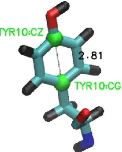
As shown in Fig.1, the transition moment of the Tyr’s side-chain lies across its aromatic plane.25 _{In the experiment, those} side chains with transition moment parallel to the orientation of the first vertical polariser will be preferentially excited. When they emit at some later time t, the orientation of these side chains will have changed due to their Brownian motion and the rotational diffusion of the protein backbone. The emitted light then can pass through the second polariser with a probability that depends on the angle between transition moment and polariser. The experimental anisotropy therefore captures the rate at which the side chains re-orientate in the sample.

Fig. 1 The Tyr side-chain

viewed using the Visual Molecular Dynamics package (VMD).28 The carbon atoms used to identify the orientation of the transition moment across the aromatic ring are labelled, and the distance in between them measured in A.

The dynamics of this molecular-scale process depends on the environment of the Tyr, so that the response with an isolated Ab1-40 monomer in solution will differ from that derived from an Ab1-40 aggregate. Similarly, the rotational diffusion of the protein backbone depends on the size of the aggregate, with larger aggregates having slower dynamics. Therefore the measurement of the fluorescence anisotropy can, in principle, be used to monitor the aggregation of Ab1-40 proteins in solution.

theoretical model of associated fluorescence decays10 _{is of the} form:

𝑟𝑒𝑥𝑝(𝑡) = 0.4 ∑2𝑖=1𝑓𝑖(𝑡). 𝑒−𝑡/𝑇𝑖, 𝑓𝑖(𝑡) = 𝛼𝑖𝑒

−𝑡/𝜏𝑖

∑2𝑖=1𝛼𝑖𝑒−𝑡/𝜏𝑖 . (1)

The components of the model are the anisotropy decays of two different states of the protein. The individual rates of the decays of the states determine the relative weights 𝑓𝑖(𝑡) in (1),

switching the total anisotropy from being dominated initially by the fast decaying state to being dominated by the slow one.

It is essential to note here that the MC and MD methods considered below can provide independent estimates of the rotational times 𝑇𝑖 which can significantly help interpretation of

the experimental anisotropy data in terms of the model given by (1).

Monte Carlo Simulations

The analysis of the anisotropy is complicated by the Tyr side-chain having a fast relaxation time as it explores its local environment, as well as a slower rotational time due to the diffusion of the monomer/oligomer that it is attached to. We explore the consequences of these timescales using MC simulations.

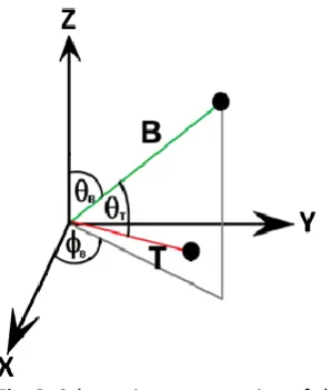
Fig. 2. Schematic representation of the vectors defined in the

system.

In order to simulate the motion of the transition moment over time, we define its orientation in terms of its angle to the backbone 𝜃𝑇 (Fig.2). The backbone itself has orientation 𝜃𝐵 to

the vertical, and a rotation of 𝜙𝐵 anticlockwise about the

vertical axis. On each MC step, these angles can change randomly at different rates. We change 𝜃𝐵 and 𝜃𝑇by randomly

chosen angles within the range ±𝑑𝜃𝐵 and ±𝑑𝜃𝑇 respectively; in

general 𝑑𝜃𝑇> 𝑑𝜃𝐵. Since we use spherical polar coordinates, 𝜙𝐵 changes by a random angle in the range ± 𝑑𝜃𝐵⁄_{sin 𝜃𝐵}. The

backbone angle movements are added to those of the transition moment. In addition, we place constraints on the allowed values of 𝜃𝑇:

𝜋

2− 𝜃𝑀< 𝜃𝑇< 𝜋 2+ 𝜃𝑀,

where 𝜃𝑀<𝜋₂, and MC steps that would violate this condition

are rejected. These constraints mimic the accessible rotamer states of the Tyr side-chain in molecular scale models.25 _There are no such constraints on the backbone movements.

Following the expression for the fundamental anisotropy of

a fluorophore,10 _{given by 𝑟0=}2

5( 3𝑐𝑜𝑠2_𝛽−1

2 ), where 𝛽 is the angle

between absorption and emission, we measure the autocorrelation from the MC simulation:

𝑟(𝑡) =2₅⟨

3(𝛽(𝑡)∙𝛽(𝑡+𝑇))2

2 −

1

2⟩_𝑇. (2)

Here time 𝑡 is measured in MC Steps, 𝛽(𝑡) is the direction of the transition moment at time t, and we average over a suitable range of times 𝑇 to observe the full 𝑟(𝑡) dynamics. In doing this, we assume that the fluorescence lifetime of the Tyr side chain is always the same throughout, and so does not affect the calculation of 𝑟(𝑡).

We fit the simulated anisotropy data of (2) to the following theoretical form:

𝑟𝑓𝑖𝑡(𝑡) = (𝑟𝑖𝑇+ 𝑟𝑖𝐵) + (𝑟0𝑇− 𝑟𝑖𝑇)𝑒

−𝑡 T𝑇

⁄ _{+ (𝑟}

0𝐵− 𝑟𝑖𝐵)𝑒

−𝑡 TB

⁄ _{. (3)}

This equation assumes that the transition moment of the Tyr will have a fast diffusion timescale 𝑇𝑇 and the backbone a larger

rotational timescale 𝑇𝐵. The values of the anisotropy at large

times t are given by the respective ‘infinity’ values 𝑟𝑖𝑇and 𝑟𝑖𝐵,

and the values at 𝑡 = 0 are 𝑟0𝑇 and 𝑟0𝐵. We also have the

constraint 𝑟0𝑇+ 𝑟0𝐵= 0.4 required by (2). Note that the

weights of the two exponential terms in (3) are time-independent, unlike the factors 𝑓𝑖(𝑡) that appear in (1); in other

words, equation (3) is a special case of equation (1).

We perform fits of (3) to both MC data and MD data described below. The five independent parameters of the fit are found by a least square error search using stochastic methods.

Molecular Dynamics Simulations

We performed fully atomistic MD simulations of single Ab1-40 as well as multi-protein systems with 2,3 or 4 Ab1-40, where the proteins start with separation of at least 3nm between them and are allowed to aggregate to form amorphous oligomers. We employ Ab1-40 for the MD simulations for comparison with our experiments; they spontaneously aggregate to form oligomers, enabling us to easily assess the effects of aggregation on the anisotropy. NAMD 2.629 _{and the Charmm27 force field was used} to perform the simulations, and VMD28 _{employed to prepare} the simulations and visualise results. We used a tcl script to obtain data on the orientation of the various Tyr transition moments (see Fig. 1).

structure for Ab1-40 was formed by removing the residues Ile41 and Ala42.

The TIP3P water model was employed with a rectilinear water box extending at least 11 Å from any protein atom. The system preparation included water minimization (1000 steps) and 100 ps water equilibration. During this stage the Langevin group based pressure control was used with a piston temperature of 300 K, and anisotropic cell fluctuations were allowed based on previous work.25 _{This was followed by a} minimization phase for the whole system (10,000 steps), then by 30 ps of heating the system to 300 K and 1 atm. pressure, and final thermal equilibration for 270 ps with time step 1 fs.

The production trajectories were performed for at least 100 ns, with a time step of 2 fs, at 300 K in the NVT ensemble. The SHAKE algorithm and Periodic Boundary Conditions were employed. Van der Waals interactions had a cut-off of 12 Å. The production MD trajectories are used to simulate the Tyr fluorescence anisotropy response on the assumption that the excited Tyr states can be represented by the ground state structure and interaction potentials. Following (2), the autocorrelation for the normalised transition moment direction

𝜇(𝑡) across the Tyr side-chain is calculated as:

𝑟(𝑡) =2₅⟨3(𝜇(𝑡+𝜏)∙𝜇(𝑡))

2

2 −

1

2⟩_𝜏. (4)

Here 𝜇(𝑡) is calculated from the coordinates of the relevant C atoms from the aromatic ring of the Tyr side-chain (see Fig. 1). In the case of multiple proteins, each Try has its own autocorrelation, and these are averaged as appropriate (the experimental anisotropy is the average of a very large number of proteins).

Results and discussion

Fluorescence Anisotropy

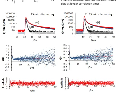
Figure 3 shows fluorescence anisotropy results 𝑟𝑒𝑥𝑝(𝑡) from a

sample of Ab1-40 taken at 15 min and 2 hr 15 min after sample preparation. Our previous research on aggregation of 50 μM Ab1-40 samples monitored by amyloid’s Tyr fluorescence decays have shown27 _{that during the initial hours after sample mixing} the aggregation is very intense, so that the anisotropy data is illustrative of the effects of this aggregation. Since the polarizers we have used absorb a high proportion of the light in the ultraviolet, the rate of data collection employed was very small. Therefore, we allowed the difference in the peak values of 𝐼∥(𝑡)

and 𝐼⊥(𝑡) to be lower than in regular fluorescence experiments

Fig. 3 Fluorescence anisotropy of Ab1-40 measured at times: (a) 00hr 15m; and (b) 02hr 15min after the sample preparation. In each case we present 𝐼∥(𝑡) and 𝐼⊥(𝑡), 𝑟𝑒𝑥𝑝(𝑡) and the residuals to the 2 exponential fits described in the text. (Karina we need to label

the columns (a) and (b).

The anisotropy performance shown in Fig. 3 is consistent with the associated anisotropy decays observed in many other aggregating systems10_{. The 𝑟𝑒𝑥𝑝}(𝑡) _{shows fast decrease on ns} timescale, followed by a gradual increase at later times. The theoretical form of equation (1) accounts for this behaviour by assuming that the observed decays are the compilation of the fluorescence decays of at least two Ab1-40 subsystems, each showing its own fluorescence lifetime 𝜏𝑖 and individual

rotational time Ti. This causes a switch in the relative

contribution of the states to the anisotropy and the growth of the slower state’s contribution. The recovered experimental curves (Fig.3) demonstrate a two-exponential character with the characteristic negative pre-exponential factors which reflect the increases in 𝑟𝑒𝑥𝑝(𝑡) at longer times. The full set of

anisotropy parameters is shown in Table 1.

Table 1. Parameters of the fluorescence anisotropy model

rexp(t)=A+B1exp[-t/T1]+ B2exp[-t/T2] fitted to the Ab1-40 data obtained in measurements that started 15 min and 135 min after sample mixing.

Age of Ab1-40 /min

A B1 B2 T1/ns T2/ns 2

15 0.111

0.003

0.384

0.002

-0.059

0.003

0.687

0.007

16.76

0.52

1.094

135 0.353

0.009

0.345

0.002

-0.287

0.009

0.693

0.007

120.6

85.5

0.996

Monte Carlo Simulations

MC simulations are performed in order to help understand the fluorescence anisotropy data of Fig. 3, and in order to aid interpretation of the MD data presented below. In these simulations, we have three parameters to select, namely the maximum angular step size 𝒅𝜽𝑩 and 𝒅𝜽𝑻for the backbone and

transition moment respectively, and the maximum allowed angle 𝜽𝑴between the normal to the backbone and the

transition moment.

We can choose these parameters to mimic the behaviour of an isolated monomer, where the transition moment moves more rapidly than the backbone and is relatively unconstrained, and values we use here are given in Table 2. We also show results from a different set of parameters that mimic the behaviour we anticipate for an oligomer of aggregated protein, where the motion of the backbone is slower and the transition moment of the Tyr side-chain more constrained. The parameters we use for this scenario are also shown in Table 2.

Table 2. MC parameters used to mimic the behaviour of a

monomer and protein aggregate.

Species 𝑑𝜃𝐵 𝑑𝜃𝑇 𝜃𝑀

Monomer 1° 5° 65°

Oligomer 0.5° 5° 25°

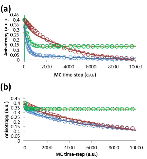
The results of the MC simulations are displayed in Fig. 4. Consider first the anisotropy calculated for the transition moment when it moves but the backbone is frozen (the green curves in Fig. 4). For the monomer simulation (Fig. 4a) we see that the anisotropy rapidly decreases over the first 1000 or so MC steps from its initial value of 0.4 to plateau at ~0.14. The reason for this is the constraint that is placed on the angular movement of the transition moment by setting 𝜃𝑀= 65°. Since

the backbone is not moving, there is a limit to the extent the transition moment can diffuse from its position at some time 𝜏 to that at a later time 𝜏 + 𝑡. We thus see how the constraining the movement of the transition moment can lead to a nonzero long-time fluorescence anisotropy. When we make the constraint on the transition moment movement very tight, as in Fig. 4b where 𝜃𝑀= 25°, there is a much smaller drop in the

anisotropy (to ~0.34) with time when the backbone is stationary.

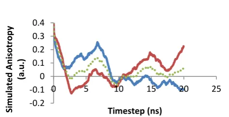
Fig. 4 Anisotropy curves from MC simulations: typical monomer

movements is shown as a solid blue line, with the transition moment only as a green line, and with backbone only as a red line. The fits to (3) are shown as open circles with colours matching the respective MC data.

Consider now the movements of the backbone, when the transition moment of the Tyr side chain remains at a constant angle to it (the red curves in Fig. 4). In this case the anisotropy does decay to approximately zero for the monomer. However, when we allow both the transition moment and the backbone to move, the resulting anisotropy is a combination of both effects. We see a rapid decrease in the anisotropy at early times, limited by the constraint imposed by 𝜃𝑀, added to the slow

decay of the backbone. In the case of the oligomer, the backbone diffusion is slow compared to the sampling window of the anisotropy, which results in an apparent nonzero long-time anisotropy.

In Fig.4 we also display the results of fitting equation (3) to the MC data, and in Table 3 we present the parameters of the fit. As can be seen, the plateau values (𝑟𝑖𝑇+ 𝑟𝑖𝐵) when the

backbone is frozen for the monomer simulation is indeed determined to be 0.14. The time-scale of the relaxation caused by the more rapid movement of the transition moment is an order of magnitude shorter than that for the backbone, whether only one type of movement is permitted (backbone-only) or both. The reason for this is that the transition moment explores its constrained parameter space (±65°) in ~1000 so random MC steps with 𝑑𝜃𝑇= 5°, whereas the backbone will

take up to ~10,000 random steps to explore its parameter space (±90°) with 𝑑𝜃𝐵= 1° in order to reduce its autocorrelation to

zero.

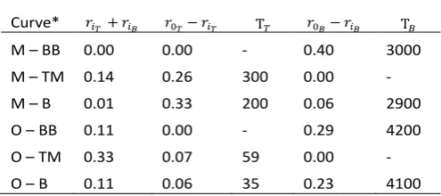
Table 3 Parameters from the fit of equation (3) to the MC

anisotropy curves of Fig. 4. The times T𝑇 and T𝐵 are given in

units of MC steps.

Curve* 𝑟𝑖𝑇+ 𝑟𝑖𝐵 𝑟0𝑇− 𝑟𝑖𝑇 T𝑇 𝑟0𝐵− 𝑟𝑖𝐵 T𝐵

M – BB 0.00 0.00 - 0.40 3000

M – TM 0.14 0.26 300 0.00 -

M – B 0.01 0.33 200 0.06 2900

O – BB 0.11 0.00 - 0.29 4200

O – TM 0.33 0.07 59 0.00 -

O – B 0.11 0.06 35 0.23 4100

*M – monomer, BB-backbone, TM – transition moment, B – both, O - oligomer

The parameters of the fit for the oligomer simulation follow the same pattern. The relaxation time T𝐵≈ 4000 is larger than

for the monomer system, since the maximum step size 𝑑𝜃𝐵= 0.5° is half that used for the monomer simulation. The smaller value of T𝑇~50 reflects the smaller parameter space (±25°) it

explores to make a small contribution to the anisotropy of the

full simulation with both transition moment and backbone movements.

The conclusions we draw from these MC results are: 1. The more rapid movement of the Tyr side-chain

transition moment will be evident in the initial rapid decline in the anisotropy;

2. The extent of this decline is determined by the level of constraint placed on its movement with respect to the backbone;

3. The slower backbone movement will be observed in the longer time relaxation of the anisotropy;

4. For the anisotropy to plateau at a nonzero value at very long times, the slow relaxation time of the backbone must either be beyond the measurement window (be that experimental or from simulation), or the backbone itself might be constrained.

In the following sections we use the perspective these conclusions provide to discuss the MD simulation results.

Molecular Dynamics Simulations Monomer Anisotropy

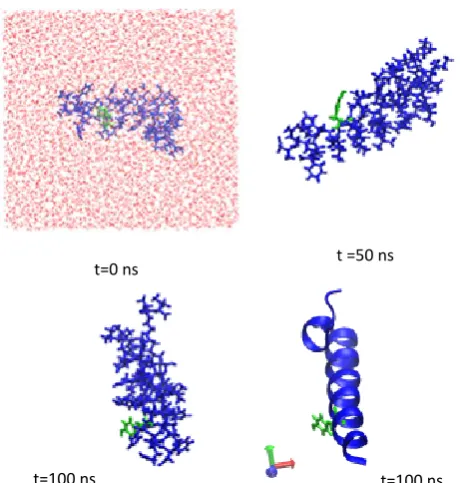
the backbone (in blue) and the tyrosine (in green) are observed to freely diffuse and fluctuate in position.

t=0 ns t =50 ns

t=100 ns t=100 ns

Fig. 5 The evolution of the Ab1-40 monomer in the MD trajectory.

The left-hand panel shows the protein conformation at the start of the trajectory (t=0 ns), along with the water molecules in red to indicate the size of the water box used. The protein atoms are in blue, and Tyr side-chain in green. The middle panels show the evolving conformation at t=50 ns and t=100 ns respectively. The right-hand panel displays the structure at t=100 ns using VMD’s ribbon representation of the secondary structure, along with the Try side-group in green as before.

The anisotropy calculated from the monomer trajectory is shown in Fig. 6, where we see behaviour that we can interpret from the MC simulations above. The transition moment appears to rotate quite freely on a ns timescale, and the anisotropy decays to approximately zero, although large fluctuations are seen in this single system. This means that the conformation of the Tyr side-group relative to the backbone does not appear to be constrained in this monomer. It is apparent that the anisotropy is dominated by the single fast timescale of the Tyr side-group, with the slow rotation of the backbone making no contribution of significance.

Fig. 6 The anisotropy (solid line) calculated from the monomer

trajectory of Fig. 5. The open circles are from the fit to Eqn. 3.

Dimer Anisotropy

The evolution of a two-protein system is illustrated in Fig. 7. The trajectory starts with two Ab1-40 proteins separated by about 3 nm. Subsequently they diffuse to interact with one another after ~26 ns, forming a stable dimer after ~50 ns. Therefore we calculated the anisotropy for this system for two separate time periods; the first period with monomers, and then the remainder for the stable dimer.

In Fig. 8 the anisotropy calculated for both monomers A (blue) and B (red) prior to aggregating is shown. The anisotropies are very different from each other; monomer B’s initially decreases sharply, temporarily levels out at approximately 10ns then starts to increase rapidly. In contrast monomer A has a sharp initial decay followed by an increase before dropping to approximately zero. These results illustrate the stochastic nature of the simulated anisotropy, where individual results taken from finite duration trajectories are prone to fluctuations. This is especially problematic in simulations with multiple proteins, whereby they can influence one another’s motion before directly forming oligomers. Nevertheless, by averaging the behaviour we get a better assessment of the anisotropy expected in a large samples simulated for long times, which provides a better point of comparison to experimental systems. The average of these two monomer’s anisotropy is also shown in Fig. 8, and is more comparable to the single monomer results of Fig. 6.

-0.2 0 0.2 0.4 0.6

0 10 20 30 40

A

n

isot

ro

p

y

t=0 ns t=26.3 ns

t=52 ns t=100 ns

Fig. 7 MD images, taken at the indicated trajectory times,

showing the aggregation of two monomers to form a tightly bound dimer. The two Ab1-40 are illustrated as VMD ribbons (one red and one blue) surrounded by the van der Waals spheres of the component atoms to show more clearly the points of interaction. The Tyr side-group is green, and for clarity the water is not shown.

Fig. 8 The MD simulated anisotropy of two monomers prior to

aggregation. Monomer A in blue, monomer B in orange and the average is the dotted line.

The anisotropy calculated during the second half of the two-monomer system is shown in Fig. 9. The two two-monomers have aggregated together to form a fairly stable dimer that is able to diffuse and rotate while maintaining the area of contact between the component monomers (see Fig. 7). This anisotropy can be interpreted in terms of the results seen for the MC simulations above; there is a much slower decay when compared to both the single protein system and this dimer system pre-aggregation. Furthermore, the plateau value apparent for monomer A is indicative of the constrained movement of its Try side-group, which is trapped by its own hydrophobic tail (residues 1-7 that are not part of the alpha-helix structure of the monomeric Ab1-40) and cannot move freely. Also, the Tyr B (on the red protein) is interacting with monomer A’s backbone.

Fig. 9 The anisotropy of the dimer formed by the aggregation of

two monomers during the MD trajectory. Monomer A in blue, monomer B in orange and the average is the dotted line.

Tetramer Anisotropy

The evolution of a four Ab1-40 simulation is illustrated in Fig. 10. The proteins start with a separation of at least 1nm and diffuse freely in the trajectory to interact with one another. Within 20 ns a tetramer starts to form. However, the initial aggregate is not stable and it soon breaks apart. It is interesting to note that the two monomers forming a dimer at 48 ns, A (blue) and B (red) in Fig. 10, are not the pair that initially formed a dimer at 13 ns (A and C, grey). This early dimer was also joined by monomer D (yellow) at 17 ns, and yet the aggregate still dissociated implying that there is a preferred mode of interaction to form stable aggregates. The preference seems to be for alignment of neighbouring alpha-helix structures, as is also apparent in Fig. 7 for the dimer, although further analysis is required in future work. After several temporary aggregation events, a stable tetramer formed at 56 ns. This aggregate then continued to compact into the tighter oligomer observed at 100 ns.

When the aggregate has fully formed, the Tyr side-chain of monomer A has its movement constrained by monomer B’s backbone. Monomer B’s Tyr is also facing monomer A’s backbone. However, unlike monomer A, monomer B has the distinct feature of being aggregated at only one end of its alpha-helix, which provides some freedom for its backbone to move and pivot about this interaction site Meanwhile monomer C is responsible for holding monomer A in place, and is also aggregated to monomer D. Monomer C’s Tyr side-chain has a lot of freedom throughout the simulation; it repeatedly opens out to the surrounding water before retracting to the protein surface. Monomer C’s backbone is restricted as it is aggregated to two other monomers from either side. Monomer D is similar to C, but it’s Tyr side-chain does not possess the same freedom of movement.

-0.2 -0.1 0 0.1 0.2 0.3 0.4

0 5 10 15 20 25

Si

m

u

late

d

An

isot

ro

p

y

(a.

u

.)

Timestep (ns)

0 0.1 0.2 0.3 0.4 0.5

0 10 20 30 40

Si

m

u

late

d

A

n

isot

ro

p

y (

a.u

.)

t=17 ns t=28 ns

t=48 ns t=56 ns

Fig. 10 MD images, taken at

the indicated trajectory times, showing the aggregation of four

monomers to form a tightly bound tetramer. The four Ab1-40 are illustrated as VMD ribbons (A blue, B red, C grey and D orange) surrounded by the van der Waals spheres of the component atoms to show more clearly the points of interaction. The Tyr side-group is green, and for clarity the water is not shown.

The anisotropy results for each monomer’s Tyr transition moment are shown in Fig. 11. Monomer A, having both its backbone and tyrosine heavily restricted throughout the simulation, has a very slow anisotropy decay and a high long-time plateau value due to the slow diffusion of the tetramer that has a time-scale beyond the ~30 ns time-averaging window accessible to these 100 ns trajectories. Similarly, monomer B’s Tyr side-chain anisotropy shows significant signs of restricted movement due to the trapping effect of monomer A’s backbone in the aggregate. The anisotropy curves for monomers C and D are similar to that of isolated monomers. The Tyr side chains of these monomers retain more freedom in their movements.

Fig.11 The anisotropy of the Tetramer formed by the

aggregation of four monomers during the MD trajectory. Monomer A in blue, monomer B in orange, monomer C in grey, monomer D is yellow and the average is the dotted line.

Comparison between Monomer and Oligomer Anisotropy

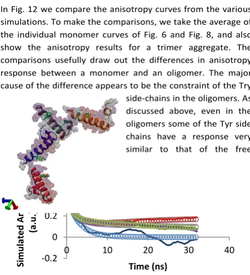
In Fig. 12 we compare the anisotropy curves from the various simulations. To make the comparisons, we take the average of the individual monomer curves of Fig. 6 and Fig. 8, and also show the anisotropy results for a trimer aggregate. The comparisons usefully draw out the differences in anisotropy response between a monomer and an oligomer. The major cause of the difference appears to be the constraint of the Try side-chains in the oligomers. As discussed above, even in the oligomers some of the Tyr side chains have a response very similar to that of the free

monomer, and only those whose movement is severely restricted display significantly different behaviour.

Fig. 12 Comparison between the anisotropy of monomers and

various oligomers: monomer (black), dimer (red), trimer (purple) and tetramer (green). The MD data is displayed as a solid line, and the best fit curves from (3) are open circles with matching colours.

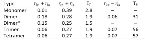
In Fig. 12 we also show the results for the fit to equation (3), and the fitting parameters are reported in Table 4. Here we see that, as might be expected, the anisotropy of the monomer is dominated by a single time-scale exponential decay reflecting the relatively free movement of the Tyr side chain. However, the larger trimer and tetramer aggregates also show evidence of a second, slower anisotropy decay on the timescale approaching that of the trajectory duration. This also leads to a nonzero long-time plateau value for the anisotropy. This behaviour is readily understandable in light of the MC data presented above, where slow rotation of the backbone is evident in conjunction with restricted Tyr side chain movements.

-0.2 -0.1 0 0.1 0.2 0.3 0.4

0 10 20 30 40

Si

m

u

lated

Ani

sotr

op

y

(a.u

.)

Timestep (ns)

-0.2 0 0.2 0.4 0.6

0 10 20 30 40

Si

m

u

late

d

An

isot

ro

p

y

(a.u

.)

Table 4. Parameters from the fit of (3) to the various MD

anisotropy curves. The times T𝑇 and T𝐵 are in ns.

Type 𝑟𝑖𝑇+ 𝑟𝑖𝐵 𝑟𝑖𝑇+ 𝑟𝑖𝐵 T𝑇 𝑟0𝐵− 𝑟𝑖𝐵 T𝐵

Monomer 0.01 0.39 2.8 – –

Dimer 0.18 0.28 1.9 0.06 31

Dimer* 0.15 0.25 1.5 – –

Trimer 0.06 0.27 1.9 0.07 56

Tetramer 0.06 0.27 1.9 0.07 57

*Fit performed with one exponential term.

The behaviour of the dimer is anomalous in that its long-time anisotropy increases rather than decays, and the fit reflects this with a negative value for the amplitude of the slow response. However, we expect that this is due to the relatively short trajectory duration for the dimer once it has formed (~50 ns, see above), and that sampling from a longer trajectory would remove this feature in the anisotropy. Indeed, performing the fit with only one exponential retains the essential features displayed by the other oligomers, and as Fig. 12 shows, the behaviour of the dimer is more in line with the larger oligomers than the monomer.

Conclusions

We have explored the use of fluorescence anisotropy as a probe of the in vitro early-stage aggregation of Ab1-40. The experimental anisotropy decays from its initial value of 0.4 on a timescale of ~4 ns to then increase again to reach a maximum on a 50 ns timescale. The time here refers to the delay between excitation and emission, and therefore probes the diffusive motion of the Tyr side chain responsible for the fluorescence. The fact that the anisotropy does not smoothly decay to zero indicates that the Ab1-40 have aggregated so that the Tyr diffusion is different to that of monomeric Ab1-40.

In order to understand better the molecular-scale cause of the anisotropy, we have used two simulation approaches. First we conducted simple MC simulations to mimic the diffusive motion of a side chain attached to a larger backbone. We find that we reproduce the competing timescales of the anisotropy curve by constraining the range of angular movement of the side chain while allowing for the slower angular diffusion of the backbone. This shows that the experiment provides evidence of the altered Try environment.

To provide a more direct molecular interpretation we also performed fully atomistic simulations of Ab1-40 monomers and oligomers. The simulated anisotropy of these species shows that the monomer anisotropy will decay smoothly to zero, whereas those for Tyr side chains within oligomers can reproduce the main features of the experimental results with the two differing timescales. In particular, the MD simulations show the importance of the Tyr movement constraint on the resulting anisotropy, in line with our conclusions from the MC simulations.

An interesting feature of our results is the reasonably good agreement between the timescales we find for the anisotropy decays. The short timescale response is caused by the diffusive motion of the Tyr side chain in the MD, and the long timescale plateau by the slow diffusion of the backbone combined with the constrained Tyr motion. This agrees well with our intuition for the experimental results. However, we note that the anisotropy reported here does not appear to be sensitive to the size of the oligomer; the trimer anisotropy is very similar to the tetramer, and the slower diffusion of larger aggregates is not distinguishable on a 40 ns timescale. To probe the effects of increasing oligomer size as Ab1-40 aggregation proceeds, a longer experimental window is needed, and much longer MD trajectories required. The latter is challenging in terms of computational cost, while the former is also difficult since aggregation opens up new inter-Tyr energy transfer mechanisms (which we have assumed to be negligible in this work) that serve to diminish the light available for fluorescence anisotropy measurements.

In conclusion, we have shown how fluorescence anisotropy does probe the early stages of Ab1-40 aggregation, and have been able to interpret this in terms of the diffusion of the fluorescent Tyr side chains. In order to follow the aggregation through a hierarchy of oligomer sizes, future work could focus on the aggregation of smaller peptides that contain a Tyr residue. The smaller size would allow simulations to probe oligomer rotation on a computationally accessible timescale, aiding the interpretation of experiments to follow the evolution of the anisotropy as the aggregation proceeds.

Conflicts of interest

Acknowledgements

The MD simulations were performed on the EPSRC funded ARCHIE-WeSt High Performance Computer (www.archie-west.ac.uk); EPSRC grant no. EP/K000586/1. OM was supported by a University of Strathclyde studentship.

Notes and references

1 R. Bradbury and M. A. Brodney, Topics in Medicinal Chemistry. Alzheimer's Disease, Springer, 2010.

2 M. Guerchet, M. Prina and M. Prince, World Alzheimer Report 2013: Journey of Caring: An analysis of long-term care for dementia,

King's College London, 2013.

3 S. Bedrood, Y. Li, J. M. Isas, B. G. Hegde, U. Baxa, I. Haworth and R. Langen, J. Biol. Chem., 2012, 297, 5235-5241.

4 W. R. Markesbery, Free Radic. Biol. Med., 1997, 23, 134-147. 5 J. C. Stroud, C. Liu, P. K. Teng and D. Eisenberg, Proc. Natl. Acad.

Sci., 2012, 109, 7717-7722.

6 V. A. Wagoner, M. Cheon, I. Chang and C. K. Hall, Proteins, 2014, 82, 1469–1483.

8 A. Zykwinska, M. Pihet, S. Radji, J. Bouchara and S. Cuenot,

Biochem. Biophys. Acta, 2014, 1844, 1137-1144.

9 M. Hiltunen, T. v. Groen and J. Jolkkonen, J.Alzheimers Dis.,

2009, 18, 401-412.

10 J. R. Lakowicz, Principles of Fluorescence Spectroscopy, Springer, 2007.

11 I. T. Marsden, L. S. Minamide and J. R. Bamburg, J. Alzheimers

Dis., 2011, 24, 681-691.

12 S. Sadigh-Eteghad, M. Talebi, M. Farhoudi, S. E. Golzari, B. Sabermarouf and J. Mahmoudi, J. Med. Hypotheses and Ideas, 2014,

8, 49-52.

13 Y. Luo, B. Bolon, M. A. Damore, H. L. D. Fitzpatrick, J. Zhang, Q. Yan, R. Vassar and M. Citron, Neurobiol. Dis., 2003, 14, 81-88. 14 M. A. Bogoyevitch, I. Boehm, A. Oakley, A. J. Ketterman and R. K. Barr, Biochem. Biophys. Acta, 2004, 1697, 89-101.

15 M. Tabaton, G. P. X. Zhu, M. A. Smith and L. Giliberto, Exp.

Neurol., 2010, 221, 18-25.

16 K. Zuo, J.-S. Gong, K. Yanagisawa and M. Michikawa, J.

Neurosci., 2002, 22, 4833-4841.

17 R. Baruch-Suchodolsky and B. Fischer, Biochem., 2009, 48, 4354-4370.

18 Z.-X. Yao and V. Papadopoulos, FASEB J., 2002, 16, 1677-1679. 19 U. Igbavboa, G. Sun, G. Weisman and W. Wood, J. Neurosci., 2009, 162, 328-338.

20 B. Maloney and D. K. Lahiri, Gene, 2011, 488, 1-12.

21 J. A. Bailey, B. Maloney, Y.-W. Ge and D. K. Lahiri, Gene, 2011,

488, 13-22.

22 S. Soscia, J. Kirby, K. Washicosky, S. Tucker, M. Ingelsson, B. Hyman, M. Burton, L. Goldstein, S. Duong, R. Tanzi and R. Moir, PLOS

One, 2010, 5.

23 R. Murphy, Biochim. Biophys. Acta , vol. 1768, no. 1923, 2007. 24 W.-F. Xue, A. L. Hellewell, E. W. Hewitt and S. E. Radford, Prion, 2010, 4, 20–25.

25 M. Amaro, K. Kubiak-Ossowska, D. Birch and O. Rolinski,

Methods Appl. Fluoresc., 2013, 1, 015006.

26 T.A. Smith and K.P. Ghiggino, Methods Appl. Fluoresc., 2015, 3, 022001.

27 M. Amaro, D. Birch and O. Rolinski, Phys. Chem. Chem. Phys., 2011, 13, 6434-6441.

28 W. Humphrey, A. Dalke and K. Schulten, J. Mol. Graph, 1996,

14, 33-38.

29 J. C. Phillips, R. Braun, W. Wang, J. Gumbart, E. Tajkhorshid, E. Villa, ch. Chipot, R. D. Skeel, L. Kale and K. Schulten, J Comput. Chem, 2005, 26, 1781-1802.