Multi-scale spatio-temporal analysis of human mobility

City, University of London Institutional Repository

Citation: Alessandretti, L., Sapiezynski, P., Lehmann, S. & Baronchelli, A. (2017).

This is the published version of the paper.

This version of the publication may differ from the final published

version.

Permanent repository link: http://openaccess.city.ac.uk/16791/

Link to published version: http://dx.doi.org/10.1371/journal.pone.0171686

Copyright and reuse: City Research Online aims to make research

outputs of City, University of London available to a wider audience.

Copyright and Moral Rights remain with the author(s) and/or copyright

holders. URLs from City Research Online may be freely distributed and

linked to.

City Research Online: http://openaccess.city.ac.uk/ publications@city.ac.uk

Multi-scale spatio-temporal analysis of human

mobility

Laura Alessandretti1_{, Piotr Sapiezynski}2_{, Sune Lehmann}2,3_{, Andrea Baronchelli}1

*

1 City, University of London, London EC1V 0HB, United Kingdom, 2 Technical University of Denmark, DK-2800 Kgs. Lyngby, Denmark, 3 Niels Bohr Institute, University of Copenhagen, DK-2100 KøbenhavnØ, Denmark

*Andrea.Baronchelli.1@city.ac.uk

Abstract

The recent availability of digital traces generated by phone calls and online logins has signifi-cantly increased the scientific understanding of human mobility. Until now, however, limited data resolution and coverage have hindered a coherent description of human displacements across different spatial and temporal scales. Here, we characterise mobility behaviour across several orders of magnitude by analysing*850 individuals’ digital traces sampled every*16 seconds for 25 months with*10 meters spatial resolution. We show that the dis-tributions of distances and waiting times between consecutive locations are best described by log-normal and gamma distributions, respectively, and that natural time-scales emerge from the regularity of human mobility. We point out that log-normal distributions also charac-terise the patterns of discovery of new places, implying that they are not a simple conse-quence of the routine of modern life.

Introduction

Characterising the statistical properties of individual trajectories is necessary to understand the underlying dynamics of human mobility and design reliable predictive models. A trajec-tory consists ofdisplacementsbetween locations andpausesat locations, where the individual stops and spends time (Fig 1). Thus, the distribution of waiting times (or pause durations),Δt, between movements and the distribution of distances,Δr, travelled between pauses are often used to quantitatively assess the dynamics of human mobility. For example, specific probability distributions of distances and waiting times characterise different types of diffusion processes. Thanks to the recent availability of data used as proxy for human trajectories including mobile phone call records (CDR), location based social networks (LBSN) data, and GPS trajectories of vehicles, the characteristic distributions of distances and waiting times between consecutive locations have been widely investigated. There is no agreement, however, on which distribu-tion best describes these empirical datasets.

Pioneer studies, based on CDR [1,2] and banknote records [3], found that the distribution of displacementΔris well approximated by a power-law,P(Δr)*Δr−β, (or ‘Le´vy distribution’ [4], as typically 1<β<3), and that an exponential cut-off in the distribution may control boundary effects [2]. These findings were confirmed by studies based on GPS trajectories of a1111111111 a1111111111 a1111111111 a1111111111 a1111111111 OPEN ACCESS

Citation: Alessandretti L, Sapiezynski P, Lehmann

S, Baronchelli A (2017) Multi-scale spatio-temporal analysis of human mobility. PLoS ONE 12(2): e0171686. doi:10.1371/journal.pone.0171686

Editor: Tobias Preis, University of Warwick,

UNITED KINGDOM

Received: November 14, 2016

Accepted: January 24, 2017

Published: February 15, 2017

Copyright:©2017 Alessandretti et al. This is an

open access article distributed under the terms of theCreative Commons Attribution License, which permits unrestricted use, distribution, and reproduction in any medium, provided the original author and source are credited.

Data Availability Statement: Data used to

generate Fig.3, Fig.5, Fig.6 and Fig.7 can be found athttps://figshare.com/s/f424d0c0d1721365950d

individuals [5–7] and vehicles [8,9], as well as online social networks data [10–12]. It has been noted, however, that power-law behaviour may fail to describe intra-urban displacements [13]. Other analyses, based on online social network data [14–16] and GPS trajectories [17–20] showed that the distribution of displacements is well fitted by an exponential curve, P(Δr)*e−λΔr, in particular at short distances. Finally, analyses based on GPS on Taxis [21,22] suggested that displacements may also obey log-normal distributions,

P(Δr)*(1/Δr)e−(logΔr−μ)2/2σ2. In Ref. [6], the authors found that this is the case also for sin-gle-transportation trips.

Fewer studies have explored the distribution of waiting times between displacements,Δt, as trajectory sampling is often uneven (e.g., in CDR data location is recorded only when the phone user makes a call or texts, and LBSN data include the positions of individuals who actively “check-in” at specific places). Analyses based on evenly sampled trajectories from mobile phone call records [1,23], and individuals GPS trajectories [5,7] found that the distri-bution of waiting times can be also approximated by a power-law. A recent study based on GPS trajectories of vehicles, however, suggests that for waiting times larger than 4 hours, this distribution is best approximated by a log-normal function [24]. Several studies have highlighted the presence of natural temporal scales in individual routines: distributions of waiting times display peaks in that corresponds to the typical times spent home on a typical day (*14 hours) and at work (*3−4 hours for a part-time job and*8−9 hours for a full-time job) [23,25,26].

Fig 2andTable 1compare distributions obtained using different data sources. The spec-trum of results reflects the heterogeneity of the considered datasets (seeFig 2). It is known in fact that data spatio-temporal resolution and coverage has an important influence on the results of the analyses performed [27–29].

Fig 1. Example of an individual trajectory. An individual trajectory is composed of pauses (red dots) and displacements (dashed black line). The trajectory shows the positions of one individual across 26 hours. Location is estimated from individual’s WiFi scans as detailed in the text and the data is sampled in 1 min bins. Red dots correspond to locations where the individual spent more than 10 consecutive minutes. The coordinates of these locations have been slightly altered to protect the subject privacy. The map was generated with the Matplotlib Basemap toolkit for Python (https://pypi.python.org/pypi/basemap). Map data©OpenStreetMap contributors (License:http://www.openstreetmap.org/copyright). Map tiles by Stamen Design, under CC BY 3.0.

doi:10.1371/journal.pone.0171686.g001 confidentiality agreement, and agree to work under

our supervision in Copenhagen. Please direct your queries to Sune Lehmann, the Principal Investigator of the Copenhagen Network Study, at

sljo@dtu.dk.

Funding: This work was supported by Villum

Foundation,http://villumfoundation.dk/ C12576AB0041F11B/0/

4F7615B6F43A8EA5C1257AEF003D9930? OpenDocument, Young Investigator programme 2012, High Resolution Networks (SL) and University of Copenhagen,http://dsin.ku.dk/news/ ucph_funds/, through the UCPH2016 Social Fabric grant (SL). The funders had no role in study design, data collection and analysis, decision to publish, or preparation of the manuscript.

Competing interests: The authors have declared

First, the datasets considered have differentspatial resolution and coverage, and few studies have so far considered the whole range of displacements occurring between*10 and 107m (10000 km) (Fig 2). Our analysis suggests that constraining the analysis to a specific distance range may result in different interpretations of the distributions. Another difference concerns thetemporal samplingin the datasets analysed so far. Uneven sampling typical of CDR and LBSN data (i) does not allow to distinguish phases ofdisplacementandpause, since individuals could be active also while transiting between locations, and (ii) may fail to capture patterns other than regular ones [31,32], because individuals’ voice-call/SMS/data activity may be higher in certain preferred locations. Finally, studies focusing on displacements effectuated using one or severalspecific transportation modality(private car [24,33], taxi [20], public trans-portation [34], or walk [7]) capture only a specific aspect of human mobility behaviour.

In this paper, we analyse mobility patterns of*850 individuals involved in the Copenhagen Network Study experiment for over 2 years [35]. Individual trajectories are determined com-bining GPS and Wi-Fi scans data resulting in a spatial resolution of*10 m, and even sam-pling every*16 s. Trajectories span more than*107m. Previous studies with comparable spatial coverage (Fig 2) relied on single-transportation modality data [8], unevenly sampled data [16], or small samples (32 individuals in Ref. [5]). To our knowledge, the Copenhagen Network Study data has the best combination of spatio-temporal resolution and sample size among the datasets analysed in the literature to date (seeMethods).

Results

We consider an individual to bepausingwhen he/she spends at least 10 consecutive minutes in the same location, andmovingin the complementary case. In the following, we refer to loca-tionsas places where individuals pause. The distribution of displacements is robust with respect to variations of the pausing parameter (seeS1 Filefor the results obtained with 15 and 20 minutes pausing).

We start by considering the three distributions most frequently reported in the literature (Table 1), namely

• The log-normal distributionof a random variablex, with parametersσandμ, defined forσ> 0 andx>0, with probability density function:

PðxÞ ¼ ffiffiffiffiffiffiffiffiffiffi1

2ps2 p

xe 1 2

ðlogxmÞ2

s2 _ð1Þ

• The Pareto distribution(i.e.power-law) of a random variablex, with parameterβ, defined for x1, andβ>1, with probability density function:

PðxÞ ¼ ðb 1ÞðxÞ b ð2Þ

Fig 2. The distribution of displacements P(Δr): heterogeneity of results found in the literature. Each horizontal line corresponds to a different dataset.

Lines extend from the minimumΔr (i.e. the spatial resolution of the data or the minimum value considered for the fit of the distribution), to the maximal length

of displacement considered (both in meters). Colours correspond to the model fitting P(Δr) according to the study reported at the end of each line. If the

distribution is not unique, but varies for different ranges ofΔr, the line is divided in segments. Lines are marked with ‘’ if the corresponding data is modelled as a sequence of two distributions of the same type with different parameters, for different rangesΔr. Refs [2,6,18,30] analyse more than one dataset. In [13] the authors analyse the same dataset for different rangesΔr. A more detailed table is presented in section “Related Work”.

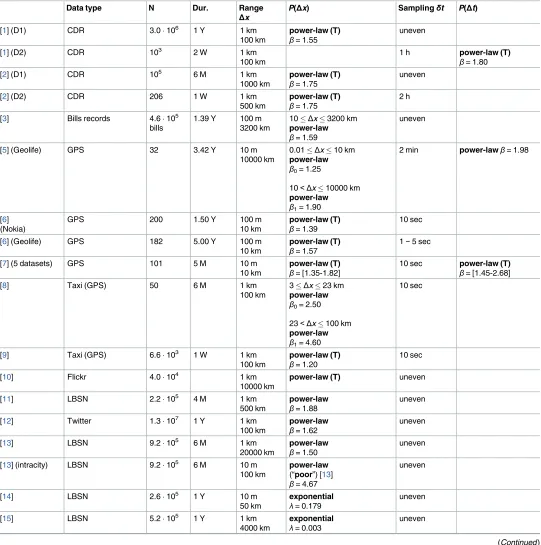
Table 1. Distribution of waiting times and displacements: A comparison of over 30 datasets on human mobility. The table reports for each dataset: the reference to the journal article/book where the study was published, the type of data (LBSN stands for Location Based Social Networks, CDR for Call Detail Record), the number of individuals (or vehicles in the case of car/taxi data) involved in the data collection, the duration of the data collection (M!months, Y

!years, D!days, W!weeks), the minimum and maximum length of spatial displacements, the shape of the probability distribution of displacements with the corresponding parameters, the temporal sampling, the shape of the distribution of waiting times with the corresponding parameters. Power-law (T), indi-cates a truncated power-law. The table can also be found athttp://lauraalessandretti.weebly.com/plosmobilityreview.html.

Data type N Dur. Range

Δx

P(Δx) Samplingδt P(Δt)

[1] (D1) CDR 3.0106 1 Y 1 km

100 km

power-law (T)

β= 1.55

uneven

[1] (D2) CDR 103 _{2 W 1 km}

100 km

1 h power-law (T)

β= 1.80

[2] (D1) CDR 105 _{6 M 1 km}

1000 km

power-law (T)

β= 1.75

uneven

[2] (D2) CDR 206 1 W 1 km

500 km

power-law (T)

β= 1.75

2 h

[3] Bills records 4.6105 bills

1.39 Y 100 m 3200 km

10Δx3200 km power-law

β= 1.59

uneven

[5] (Geolife) GPS 32 3.42 Y 10 m

10000 km

0.01Δx10 km power-law

β0= 1.25

10< Δx10000 km power-law

β1= 1.90

2 min power-lawβ= 1.98

[6] (Nokia)

GPS 200 1.50 Y 100 m

10 km

power-law (T)

β= 1.39

10 sec

[6] (Geolife) GPS 182 5.00 Y 100 m

10 km

power-law (T)

β= 1.57

1−5 sec

[7] (5 datasets) GPS 101 5 M 10 m

10 km

power-law (T)

β= [1.35-1.82]

10 sec power-law (T)

β= [1.45-2.68]

[8] Taxi (GPS) 50 6 M 1 km

100 km

3Δx23 km power-law

β0= 2.50

23< Δx100 km power-law

β1= 4.60

10 sec

[9] Taxi (GPS) 6.6103 _{1 W 1 km}

100 km

power-law (T)

β= 1.20

10 sec

[10] Flickr 4.0104 _{1 km}

10000 km

power-law (T) uneven

[11] LBSN 2.2105 _{4 M 1 km}

500 km

power-law

β= 1.88

uneven

[12] Twitter 1.3107 _{1 Y 1 km}

100 km

power-law

β= 1.62

uneven

[13] LBSN 9.2105 _{6 M 1 km}

20000 km

power-law

β= 1.50

uneven

[13] (intracity) LBSN 9.2105 _{6 M 10 m}

100 km

power-law (“poor”) [13]

β= 4.67

uneven

[14] LBSN 2.6105 1 Y 10 m

50 km

exponential

λ= 0.179

uneven

[15] LBSN 5.2105 1 Y 1 km

4000 km

exponential

λ= 0.003

uneven

Table 1. (Continued)

Data type N Dur. Range

Δx

P(Δx) Samplingδt P(Δt)

[16] Twitter 1.6105 8 M 10 m

4000 km

0.01Δx0.1 km exponential

λ= 0.073

0.1< Δx100 km Stretched power-law

β1= 0.45

100< Δx4000 km power-law

β2= 1.32

uneven

[17] Taxi (GPS) 803 1.25 Y 1 km

100 km

Δx15 km exponential

λ= 0.36

15< Δx100 km power-law

β= 3.66

30 sec

[18] (D1) Taxi (GPS) 104 3 M 1 km

100 km

1Δx20 km exponential

λ0= 0.23

20< Δx100 km exponential

λ1= 0.17

1 min

[18] (D2) Taxi (GPS) 104 _{2 M 1 km}

100 km

1Δx20 km exponential

λ0= 0.24

20< Δx100 km exponential

λ1= 0.18

1 min

[19] Taxi (GPS) 6.6103 _{1 W 2 km}

20 km

exponential

λ= [0.072-0.252]

10 sec

[20] (3 datasets)

Taxi (GPS) 104 _{1 M 600 m}

10 km

exponential [9−177] s power-law

[21] (6 datasets)

Taxi (GPS) 3.0104 _{[1 M-2 Y] 1 km}

100 km

log-normal

μ= [0.77-1.32],

σ= [0.67-0.87]

[24−116] s

[22] Taxi (GPS) 1.1103 6 M 100 m

30 km

log-normal

μ= 0.38,

σ= 0.48

30 sec

[23] Surveys 104 1 Y self-reported power-law (T)

β= 0.49 [24] Private Cars (GPS) 7.8105 1 M 1 km

500 km

superimposition Poisson 10 sec Δt4h power-law

β= 1.03

1Δt200h log-normal

μ= 1.60,

σ= 1.60 [26] Private Cars (GPS) 3.5104 _{1 M 300 m}

100 km

polynomial 10 sec power-law

β= 0.97

• The exponential distributionof a random variablex, with parameterλ, wherex0, andλ> 0, with probability density function:

PðxÞ ¼le lx _ð3Þ

InEq (2)the probability density can be shifted byx0and/or scaled bys, asP(x) is identically

equivalent toP(y)/s, withy¼ðx x0_s Þ. In Eqs (1) and (3),P(x) is identically equivalent toP(y), withy= (x−x0). In this work, the shift (x0) and scale (s) parameters are considered as

addi-tional parameters to take into account the data resolution. With few exceptions, the results pre-sented below hold also imposing no shift,x0= 0 (seeS1 File). Note also that Pareto

distributions with exponential cut-off (or truncated Pareto) are considered below (see also Table 1).

Distribution of displacements

We start our analysis by investigating the distribution of displacements between consecutive stop-locationsP(Δr). First, we consider the overall distribution of the displacementsΔrusing all available data (851 individuals over 25 months). We find thatP(Δr) is best described by a log-normal distribution (Eq (1)) with parametersμ= 6.78±0.07 andσ= 2.45±0.04, which maximises Akaike Information Criterion (seeMethods)—among the three models considered —with Akaike weight*1 (Fig 3, see alsoS1 File).

Second, we investigate if this results holds also for sub-samples of the entire dataset. We bootstrap data 1000 times for samples of 200 and 100 individuals, and we verify that the best distribution is log-normal for all samples, and the average parameters inferred through the bootstrapping procedure are consistent with the parameters found for the entire dataset (see S1 File). In fact, the errors on the value of the parameters reported above are computed by

Table 1. (Continued)

Data type N Dur. Range

Δx

P(Δx) Samplingδt P(Δt)

[30] (D1) CDR 1.3106 1 M 1 km

200 km

power-law

β= 2.02

uneven

[30] (D2) CDR 6106 1 Y 1 km

500 km

power-law

β= 1.75

uneven

[30] (D3) CDR 4 Y 1 km

100 km

power-law

β= 1.80

uneven

[34] Travel cards 2.0106 1 W 100 m

50 km

negative binomial

μ= 9.28,

σ= 5.83

uneven

[42] Travel

Diaries

230 1.5 M 1 km

400 km

power-law (T)

β= 1.05

self-reported

[56] Private Cars (GPS) 7.5104 1 M 10 m 500 km

0.01Δx20 km exponential

20< Δx150 km power-law

β1= 3.30

30 sec Δt3h exponential

λ= 1.02

[57] Taxi (GPS) 1 D 200 m

1000 km

power-law

β= 2.70

bootstrapping data for samples of 100 randomly selected individuals. This analysis ensures homogeneity within the population considered, and takes into account also that often smaller sample sizes were analysed in previous literature.

Third, we zoom in to the individual level. We find that the individual distribution of dis-placements is best described by a log-normal function for 96.2% of individuals. The best distri-bution is the Pareto distridistri-bution for 1.4%, and exponential for the remaining 2.4%. However, the number of data points per individual tend to be significantly lower in group of individuals exhibiting Pareto or exponential distributions, so that one should be cautious in interpreting the observed deviations from a log-normal distribution.Fig 4reports the histogram of the individualμparameters for the 96.2% of the population that is best described by a log-normal distribution, along with three examples of individual distributions.

Finally, we look at largeΔrin order to compare our results with precedent studies relying on data with larger spatial resolution. We find that limiting the analysis to large values of Δrresults in the selection of a Pareto distribution (Eq (2)). We identify the threshold Δr= 7420 m as the minimal resolution for which the best fit inΔr<Δr<107m is Pareto with coefficientβ= 1.81±0.03 and not log-normal. By bootstrapping 1000 times over samples of 100 individuals we find thatD^r ¼7488:3328:2m. Thus, power-law distributions describe mobility behaviour only for large enough distances, while mobility patterns including distances smaller than 7420 m are better described by log-normal distributions.

Fig 3. Distribution of displacements. Blue dotted line: data. Black dashed line: log-normal fit with characteristic parameterμandσ. Red dashed line: Pareto fit with characteristic parameterβforΔr>7420 m.

Distribution of waiting times

We now analyse the distribution of waiting times between displacements. The best model describing the distribution of waiting times over all individuals is the log-normal distribution (Eq (1),Fig 5, see alsoS1 File), with parametersμ=−0.42±0.04,σ= 2.14±0.02. As above, errors are found by bootstrapping over samples of 100 individuals. Also, by bootstrapping we find that the log-normal distribution is the best descriptor for samples of 200 and 100 randomly selected individuals (seeS1 File). As in the case of displacements, we find that restricting the analysis to large values of our observableΔt, and specifically considering only Δt>Δt= 13 h, results in the selection of the Pareto distribution (Eq (2), seeFig 5), with coef-ficientβ= 1.44±0.01. We find by averaging over 100 samples of 200 individuals that

^

Dt ¼13:010:12. Note that the log-normal distribution is selected as the best model also when the analysis is restricted toΔt<Δt.

Fig 4. Distribution of individual displacements. A) Frequency histogram of 96.2% of individuals for which the individual distribution of displacement is log-normal, according to the value of the log-normal fit coefficientμ. B-C-D) Examples of the distribution of displacements P(Δr) of three individuals i1(B), i2(C), i3

(D) (dotted line), with the corresponding log-normal fit (dashed line). The value of the fit coefficientsμandσare reported in each subfigure.

The distribution of waiting times shows also the existence of “natural time-scales” of human mobility. We detect local maxima of the distribution at 14.0, 39.3, 64.8, and 89.9 hours. Hence, 14 hours is the typical amount of time that students in the experiment spent home every day, in agreement with previous analyses on human mobility [23,25,26]. Other peaks appear for intervalsΔt14 +n24, withn= {2, 3. . .}, suggesting individuals spend several days at home. Notice also that the distribution we consider is limited toΔt<5 days, an interval much shorter than the observation time-window (about 2 years), a fact that guarantees the absence of possible spurious effects [29]. This limit is imposed to control the cases in which students leave their phones home. The upper bound is arbitrarily set to 5 days; however, we have verified that results are consistent with respect to variations of this choice.

Distribution of displacements between discoveries

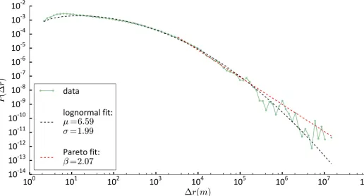
Log-normal features also characterise patterns ofexploration. We consider the temporal sequence of stop-locations that individuals visit for the first time—in our observational win-dow—and characterise the distributions of displacements between these ‘discoveries’. We find that the distribution of distances between consecutive discoveriesP(Δr) is best described as a log-normal distribution with parametersμ= 6.59±0.02,σ= 1.99±0.01, (Fig 6, see alsoS1 File). ForΔr>2800 m, the best model fitting the distribution of displacements is the Pareto distribution with coefficientβ= 2.07±0.02. This results are verified by bootstrapping (seeS1 File).

Fig 5. Distribution of waiting times between displacements. Yellow dotted line: data. Black dashed line: Log-normal fit with characteristic parameterμ

andσ. Red dashed line: Pareto fit with characteristic parameterβforΔt>13 h.

Correlations between pauses and displacements

We further investigate the properties of individual trajectories by analysing the correlations between the distanceΔrand the durationΔtdispcharacterising a displacement and the timeΔt spent at destination.Fig 7Ashows a positive correlation betweenΔrandΔtdispforΔr≳300 m (p<0.01). AsΔris the distance between the displacement origin and destination, the absence of correlation at short distances could be due to individuals not taking the fastest route. A posi-tive correlation characterises also the distanceΔrcovered between origin and destination and the waiting time at destination for distances 30 m≲Δr≲104m (p<0.01). Instead, the corre-lation is negative for distances larger than 5×104m (Fig 7B). This could suggest that individu-als break long trips with short pauses. We have verified that these results hold individu-also when individuals’ most important locations (typically including university and home) are removed from the trajectory, implying that these correlations are not dominated by daily commuting.

Further analysis: Selection of the best model among 68 distributions

In the previous sections we have restricted the analysis of the distributions of displacements and waiting times to the three functional forms that are most frequently found in the literature. We now repeat the selection procedure considering a list of 68 models (seeS1 Filefor the list of distributions) in order to confirm the results described above.

The distributions of displacements and displacements between discoveries are best described by log-normal distributions also when the choice is extended to 68 models, and tails

Fig 6. Distribution of displacements between discoveries. Green dotted line: data. Black dashed line: Log-normal fit with characteristic parameterμand

σ. Red dashed line: Pareto fit with characteristic parameterβforΔr>2800 m.

(respectively forΔr>Δr= 7420 m andΔr>Δr= 2800 m) are better modelled as generalised Pareto distribution, with form:

PðxÞ ¼ ð1þxxÞ xþx1 ð4Þ

whereξis the parameters of the model, such thatx0 ifξ0, and0x 1 xifξ<0.

The best model selected for the whole distribution of waiting time among the 68 models considered is a gamma distribution, defined forx2(0,1),k>0 andθ>0 as:

PðxÞ ¼ 1

GðkÞykx

k 1

e yx

whereGðzÞ ¼R₀1xz 1_e x_{dx. Although the gamma distribution is the best model for the} distri-bution of waiting times (seeS1 Filefor the result of the fit), the presence of natural scales could indicate that the whole distribution may be better described as the composition of several models.

Fig 7. Correlations between displacements and pauses. A) The durationΔtdispof a displacement vs the distanceΔr between origin and destination. The

blue line is the median value ofΔr andΔtdispcomputed within log-spaced 2-dimensional bins. The filled blue area corresponds to the 25-75 percentile range.

The value of the Pearson correlation coefficient within the shaded grey area indicates a positive correlation, with p−value<0.01. The dashed line is a power-law function with coefficientβ, as a guide for the eye. B) The waiting timeΔt at destination vs the distanceΔr between origin and destination. The blue line is

the median value ofΔr andΔt computed within log-spaced 2-dimensional bins. The filled blue area corresponds to the 25-75 percentile range. The value of

the Pearson correlation coefficient within the shaded grey area indicates a positive correlation, with p−value<0.01. The dashed line is a power-law function with coefficientβ, as a guide for the eye.

Discussion

Using high resolution data we have characterised human mobility patterns across a wide range of scales. We have shown that both the distribution of displacements and waiting times between displacements are best described by a log-normal distribution. We found, however, that power-law distributions are selected as the best model when only large spatial or temporal scales are considered, thus explaining (at least partially) the disagreement between previous studies. We also showed that log-normal distributions characterise the distribution of displacements between discoveries, implying that this property is not a simple consequence of the stability of human mobility but a characteristic feature of human behaviour. Finally, we have shown that there exist correlations between displacements’ length and the waiting time at destination.

The heavy tailed nature of human mobility has been attributed to various factors, including differences between individual trajectories [36], search optimisation [37–40], the hierarchical organisation of the streets network [41] and of the transportation system [6,24,42]. On the other hand log-normal distributions can result from multiplicative [43] and additive [44] pro-cesses and describe the inter-event time of different human activities such as writing emails, commenting/voting on online content [45] and creating friendship relations on online social networks [46]. Instead, the distribution of inter-event time in mobile-phone call communica-tion activity can be described as the composicommunica-tion of power-laws [47–49], a feature attributed to the existence of characteristic scales in communication activity such as the time needed to answer a call, as well as the existence of circadian, weakly and monthly patterns. We also find clear signatures of circadian patterns, which could indicate that the whole distribution may be better described as the composition of several models. However, in our case the best descrip-tion for times includingΔt<Δt_{is the gamma distribution, which thus is selected both when} the whole range of scales is considered and when the analysis is restricted to short times.

Our results come from the analysis of a sample of*850 University students, which of course represent a very specific sample of the whole population. Nevertheless, it is worth noting that many statistical properties of CNS students mobility patterns are consistent with previous results, such as the distribution of the radius of gyration, the Zipf-like behaviour of individual locations frequency-rank plot, and the power-law tail of the distribution of displacements (β= 1.81±0.03 vs.β= 1.75±0.15 of [2]). Details are reported in Supplementary Information of [50].

While identifying the mechanism responsible for the observed mobility patterns is beyond the scope of the present article, we anticipate that a more complete spatio-temporal description of human mobility will help us develop better models of human mobility behaviour [24,51]. Our findings can also help the understanding of phenomena such as the spreading of epidem-ics at different spatial resolutions, since the nature of heterogeneous waiting times between dis-placements have a major impact on the spreading of diseases [52].

Methods

Data description and pre-processing

The WiFi scans data provides a time-series of wireless network scans performed by partici-pants’ mobile devices. Each record(i, t, SSID, BSSID, RSSI)indicates:

• the participant identifier,i

• the timestamp in seconds,t

• the name of the wireless network scanned,SSID

• the unique identifier of the access point (AP) providing access to the wireless network,BSSID

• the signal strength in dBm,RSSI.

APs do not have geographical coordinates attached, but their position tend to be fixed. The geographical position of APs is estimated the procedure described inS1 File, which used par-ticipants’ sequences of GPS scans to obtainAPslocations and remove mobileAPs. Then, we clustered geo-localisedAPsto “locations” using a graph-based approach. With our definition, a “location” is a connected component in the graphGd, where a link exists between twoAPsif their distance is smaller than a thresholdd(see [50], SI for more details). Here, we present results obtained ford= 2 m. However, results are robust with respect to the choice of the threshold (see also [50]).

Throughout the experiment, participants’ devices scanned for WiFi everyΔtseconds. The median time between scans is betweenΔtM= 16 s andΔtM<60 s for 90% of the population (see also [50], SI). Data was temporally aggregated in bins of lengthΔt= 60 s, since we focus here on thepausesbetween moves. If a participant visits more than one location within a time-bin, we assign the location in which they spent the most time to that bin. Given our definition of location and the given time-binning, the median daily time coverage (the fraction of min-utes/day that an individual’s position is known, where the median is taken across all days) is included between 0.6 and 0.98 for 90% of the population.

Model selection

The best model is selected using Akaike weights [53]. First, we determine the best fit parame-ters for each of the models via Nelder-Mead numerical Likelihood maximisation [54] (maxi-misation is considered to fail if convergence with tolerancet= 0.0001 is not reached after 200Niterations, whereNis the length of the data). For each modelm, we compute the Akaike Information Criterion:

AICm¼ 2logLmþ2Vmþ

2VmðVmþ1Þ n Vm 1

ð5Þ

whereLmis the maximum likelihood for the candidate modelm,Vmis the number of free parameters in the model, andnis the sample size. TheAICreaches its minimum valueAICmin for the model that minimises the expected information loss. Thus, AIC rewards descriptive accuracy via the maximum likelihood and penalises models with large number of parameters.

The Akaikewm(AIC) weight of a modelmcorresponds to its relative likelihood with respect to a set of possible models. Measuring the Akaike weights allows us to compare the descriptive power of several models.

wmðAICÞ ¼

e 12ðAICm AICminÞ

XK

k¼1

For all distributions considered in this paper, we found one modelmsuch thatwm*1 (which implies all the other models have Akaike weight very close to 0).

Figures

All figures were generated using Matplotlib [55] package (version 1.5.3) for Python.

Related work

We present here more detailed analysis of the literature discussed in the paper.

Supporting information

S1 File. Supporting figures and tables.

(PDF)

Author Contributions

Conceptualization: LA SL AB.

Data curation: PS.

Formal analysis: LA SL AB.

Investigation: LA SL AB.

Writing – original draft: LA AB SL.

Writing – review & editing: LA PS SL AB.

References

1. Song C, Koren T, Wang P, Baraba´si AL. Modelling the scaling properties of human mobility. Nature Physics. 2010; 6(10):818–823. doi:10.1038/nphys1760

2. Gonzalez MC, Hidalgo CA, Barabasi AL. Understanding individual human mobility patterns. Nature. 2008; 453(7196):779–782. doi:10.1038/nature06958PMID:18528393

3. Brockmann D, Hufnagel L, Geisel T. The scaling laws of human travel. Nature. 2006; 439(7075):462– 465. doi:10.1038/nature04292PMID:16437114

4. Baronchelli A, Radicchi F. Le´vy flights in human behavior and cognition. Chaos, Solitons & Fractals. 2013; 56:101–105. doi:10.1016/j.chaos.2013.07.013

5. Wang XW, Han XP, Wang BH. Correlations and scaling laws in human mobility. PloS one. 2014; 9(1): e84954. doi:10.1371/journal.pone.0084954PMID:24454769

6. Zhao K, Musolesi M, Hui P, Rao W, Tarkoma S. Explaining the power-law distribution of human mobility through transportation modality decomposition. Scientific reports. 2015;5.

7. Rhee I, Shin M, Hong S, Lee K, Kim SJ, Chong S. On the levy-walk nature of human mobility. IEEE/ ACM transactions on networking (TON). 2011; 19(3):630–643. doi:10.1109/TNET.2011.2120618

8. Jiang B, Yin J, Zhao S. Characterizing the human mobility pattern in a large street network. Physical Review E. 2009; 80(2):021136. doi:10.1103/PhysRevE.80.021136

9. Liu Y, Kang C, Gao S, Xiao Y, Tian Y. Understanding intra-urban trip patterns from taxi trajectory data. Journal of geographical systems. 2012; 14(4):463–483. doi:10.1007/s10109-012-0166-z

10. Beiro´ MG, Panisson A, Tizzoni M, Cattuto C. Predicting human mobility through the assimilation of social media traces into mobility models. arXiv preprint arXiv:160104560. 2016.

11. Cheng Z, Caverlee J, Lee K, Sui DZ. Exploring Millions of Footprints in Location Sharing Services. ICWSM. 2011; 2011:81–88.

12. Hawelka B, Sitko I, Beinat E, Sobolevsky S, Kazakopoulos P, Ratti C. Geo-located Twitter as proxy for global mobility patterns. Cartography and Geographic Information Science. 2014; 41(3):260–271. doi:

13. Noulas A, Scellato S, Lambiotte R, Pontil M, Mascolo C. A tale of many cities: universal patterns in human urban mobility. PloS one. 2012; 7(5):e37027. doi:10.1371/journal.pone.0037027PMID:

22666339

14. Wu L, Zhi Y, Sui Z, Liu Y. Intra-urban human mobility and activity transition: evidence from social media check-in data. PloS one. 2014; 9(5):e97010. doi:10.1371/journal.pone.0097010PMID:24824892

15. Liu Y, Sui Z, Kang C, Gao Y. Uncovering patterns of inter-urban trip and spatial interaction from social media check-in data. PloS one. 2014; 9(1):e86026. doi:10.1371/journal.pone.0086026PMID:

24465849

16. Jurdak R, Zhao K, Liu J, AbouJaoude M, Cameron M, Newth D. Understanding human mobility from Twitter. PloS one. 2015; 10(7):e0131469. doi:10.1371/journal.pone.0131469PMID:26154597

17. Liu H, Chen YH, Lih JS. Crossover from exponential to power-law scaling for human mobility pattern in urban, suburban and rural areas. The European Physical Journal B. 2015; 88(5):1–7. doi:10.1140/epjb/ e2015-60232-1

18. Liang X, Zheng X, Lv W, Zhu T, Xu K. The scaling of human mobility by taxis is exponential. Physica A: Statistical Mechanics and its Applications. 2012; 391(5):2135–2144. doi:10.1016/j.physa.2011.11.035

19. Gong L, Liu X, Wu L, Liu Y. Inferring trip purposes and uncovering travel patterns from taxi trajectory data. Cartography and Geographic Information Science. 2016; 43(2):103–114. doi:10.1080/15230406. 2015.1014424

20. Zhao K, Chinnasamy M, Tarkoma S. Automatic City Region Analysis for Urban Routing. In: 2015 IEEE International Conference on Data Mining Workshop (ICDMW). IEEE; 2015. p. 1136–1142.

21. Wang W, Pan L, Yuan N, Zhang S, Liu D. A comparative analysis of intra-city human mobility by taxi. Physica A: Statistical Mechanics and its Applications. 2015; 420:134–147. doi:10.1016/j.physa.2014. 10.085

22. Tang J, Liu F, Wang Y, Wang H. Uncovering urban human mobility from large scale taxi GPS data. Phy-sica A: Statistical Mechanics and its Applications. 2015; 438:140–153. doi:10.1016/j.physa.2015.06. 032

23. Schneider CM, Belik V, Couronne´ T, Smoreda Z, Gonza´lez MC. Unravelling daily human mobility motifs. Journal of The Royal Society Interface. 2013; 10(84):20130246. doi:10.1098/rsif.2013.0246

24. Gallotti R, Bazzani A, Rambaldi S, Barthelemy M. A stochastic model of randomly accelerated walkers for human mobility. Nature Communications. 2016; 7:12600. doi:10.1038/ncomms12600PMID:

27573984

25. Hasan S, Schneider CM, Ukkusuri SV, Gonza´lez MC. Spatiotemporal patterns of urban human mobility. Journal of Statistical Physics. 2013; 151(1-2):304–318. doi:10.1007/s10955-012-0645-0

26. Bazzani A, Giorgini B, Rambaldi S, Gallotti R, Giovannini L. Statistical laws in urban mobility from micro-scopic GPS data in the area of Florence. Journal of Statistical Mechanics: Theory and Experiment. 2010; 2010(05):P05001. doi:10.1088/1742-5468/2010/05/P05001

27. Paul T, Stanley K, Osgood N, Bell S, Muhajarine N. Scaling Behavior of Human Mobility Distributions. In: International Conference on Geographic Information Science. Springer; 2016. p. 145–159. 28. Decuyper A, Browet A, Traag V, Blondel VD, Delvenne JC. Clean up or mess up: the effect of sampling

biases on measurements of degree distributions in mobile phone datasets. arXiv preprint arXiv:160909413. 2016.

29. Kivela¨ M, Porter MA. Estimating interevent time distributions from finite observation periods in commu-nication networks. Physical Review E. 2015; 92(5):052813. doi:10.1103/PhysRevE.92.052813

30. Deville P, Song C, Eagle N, Blondel VD, Baraba´si AL, Wang D. Scaling identity connects human mobil-ity and social interactions. Proceedings of the National Academy of Sciences. 2016; p. 201525443. 31. C¸ olak S, Alexander LP, Alvim BG, Mehndiretta SR, Gonza´lez MC. Analyzing cell phone location data

for urban trabel: current methods, limitations and opportunities. In: Transportation Research Board 94th Annual Meeting. 15-5279; 2015.

32. Ranjan G, Zang H, Zhang ZL, Bolot J. Are call detail records biased for sampling human mobility? ACM SIGMOBILE Mobile Computing and Communications Review. 2012; 16(3):33–44. doi:10.1145/ 2412096.2412101

33. Gallotti R, Bazzani A, Rambaldi S. Understanding the variability of daily travel-time expenditures using GPS trajectory data. EPJ Data Science. 2015; 4(1):1. doi:10.1140/epjds/s13688-015-0055-z

34. Roth C, Kang SM, Batty M, Barthe´lemy M. Structure of urban movements: polycentric activity and entangled hierarchical flows. PloS one. 2011; 6(1):e15923. doi:10.1371/journal.pone.0015923PMID:

35. Stopczynski A, Sekara V, Sapiezynski P, Cuttone A, Madsen MM, Larsen JE, et al. Measuring large-scale social networks with high resolution. PloS one. 2014; 9(4):e95978. doi:10.1371/journal.pone. 0095978PMID:24770359

36. Petrovskii S, Mashanova A, Jansen VA. Variation in individual walking behavior creates the impression of a Le´vy flight. Proceedings of the National Academy of Sciences. 2011; 108(21):8704–8707. doi:10. 1073/pnas.1015208108

37. Viswanathan GM, Buldyrev SV, Havlin S, Da Luz M, Raposo E, Stanley HE. Optimizing the success of random searches. Nature. 1999; 401(6756):911–914. doi:10.1038/44831PMID:10553906

38. Lomholt MA, Tal K, Metzler R, Joseph K. Le´vy strategies in intermittent search processes are advanta-geous. Proceedings of the National Academy of Sciences. 2008; 105(32):11055–11059. doi:10.1073/ pnas.0803117105

39. Raposo E, Buldyrev S, Da Luz M, Viswanathan G, Stanley H. Le´vy flights and random searches. Jour-nal of Physics A: mathematical and theoretical. 2009; 42(43):434003. doi:10.1088/1751-8113/42/43/ 434003

40. Santos M, Boyer D, Miramontes O, Viswanathan G, Raposo E, Mateos J, et al. Origin of power-law dis-tributions in deterministic walks: The influence of landscape geometry. Physical Review E. 2007; 75 (6):061114. doi:10.1103/PhysRevE.75.061114

41. Han XP, Hao Q, Wang BH, Zhou T. Origin of the scaling law in human mobility: Hierarchy of traffic sys-tems. Physical Review E. 2011; 83(3):036117. doi:10.1103/PhysRevE.83.036117PMID:21517568

42. Yan XY, Han XP, Wang BH, Zhou T. Diversity of individual mobility patterns and emergence of aggre-gated scaling laws. Scientific reports. 2013;3.

43. Mitzenmacher M. A brief history of generative models for power law and lognormal distributions. Inter-net mathematics. 2004; 1(2):226–251. doi:10.1080/15427951.2004.10129088

44. Mouri H. Log-normal distribution from a process that is not multiplicative but is additive. Physical Review E. 2013; 88(4):042124. doi:10.1103/PhysRevE.88.042124PMID:24229133

45. Van Mieghem P, Blenn N, Doerr C. Lognormal distribution in the digg online social network. The Euro-pean Physical Journal B. 2011; 83(2):251–261. doi:10.1140/epjb/e2011-20124-0

46. Blenn N, Van Mieghem P. Are human interactivity times lognormal? arXiv preprint arXiv:160702952. 2016.

47. Karsai M, Kivela¨ M, Pan RK, Kaski K, Kerte´sz J, Baraba´si AL, et al. Small but slow world: How network topology and burstiness slow down spreading. Physical Review E. 2011; 83(2):025102. doi:10.1103/ PhysRevE.83.025102

48. Jo HH, Karsai M, Kerte´sz J, Kaski K. Circadian pattern and burstiness in mobile phone communication. New Journal of Physics. 2012; 14(1):013055. doi:10.1088/1367-2630/14/1/013055

49. Krings G, Karsai M, Bernhardsson S, Blondel VD, Sarama¨ki J. Effects of time window size and place-ment on the structure of an aggregated communication network. EPJ Data Science. 2012; 1(1):1. doi:

10.1140/epjds4

50. Alessandretti L, Sapiezynski P, Lehmann S, Baronchelli A. Evidence for a Conserved Quantity in Human Mobility; 2016.

51. Gutie´rrez-Roig M, Sagarra O, Oltra A, Bartumeus F, Diaz-Guilera A, Perello´ J. Active and reactive behaviour in human mobility: the influence of attraction points on pedestrians. arXiv preprint arXiv:151103604. 2015.

52. Poletto C, Tizzoni M, Colizza V. Human mobility and time spent at destination: impact on spatial epi-demic spreading. Journal of theoretical biology. 2013; 338:41–58. doi:10.1016/j.jtbi.2013.08.032

PMID:24012488

53. Wagenmakers EJ, Farrell S. AIC model selection using Akaike weights. Psychonomic bulletin & review. 2004; 11(1):192–196. doi:10.3758/BF03206482

54. Nelder JA, Mead R. A simplex method for function minimization. The computer journal. 1965; 7(4):308– 313. doi:10.1093/comjnl/7.4.308

55. Hunter JD, et al. Matplotlib: A 2D graphics environment. Computing in science and engineering. 2007; 9 (3):90–95. doi:10.1109/MCSE.2007.55

56. Gallotti R, Bazzani A, Rambaldi S. Towards a statistical physics of human mobility. International Journal of Modern Physics C. 2012; 23(09):1250061. doi:10.1142/S0129183112500611