Modeling the effect of occupants' behavior on household carbon emissions

(1)

- 1 - 1

(2)

- 2 - Modeling the effect of occupants’ behavior on household carbon emissions

4

Dr Ibrahim Motawa1*_{and Michael Oladokun}2

5

1_{Department of Architecture, Faculty of Engineering, University of Strathclyde, Glasgow,UK}

6

2_{School of the Built Environment, Heriot-Watt University, Edinburgh, UK}

7

*Corresponding email: ibrahim.motawa@strath.ac.uk 8

9

Abstract 10

Occupants’ behavior has proven its significant impact on buildings performance. The 11

research on carbon emissions has therefore recommended the integration of the technical and 12

behavioral disciplines in order to accurately predict buildings carbon emissions. While 13

various models were developed that consider the actions of occupants based on quantitative 14

data, there are little efforts that link the impact of occupants’ behavior on selected energy 15

strategies while also consider the economic, technological, and environmental impacts. For 16

this research, a dynamic model will be developed to simulate the interaction of occupants’ 17

behavior with various energy efficient scenarios to reduce carbon emissions. The model will 18

help test the effectiveness of certain energy efficient scenarios before implementation. This 19

paper illustrates the structure and the application of the proposed model. The model results 20

show that the behavioral change can contribute enormously to the carbon emissions reduction 21

even without the installation of more energy efficient improvements. 22

23

Keywords: Household Carbon Emissions, Occupants Behavior, System Dynamics 24

(3)

- 3 - Introduction

29

Building Services Research Information Association (BSRIA) (2011) reported that the 30

currently used technology is a key reason for creating a gap between the actual and the 31

predicted performance of buildings. Mahdavi and Pröglhöf (2009), and Azar and Menassa 32

(2012) submitted that occupants’ behavior affects significantly on the dwellings performance. 33

Occupancy-focused interventions can systematically reduce energy consumption especially 34

for existing buildings where installing energy efficient technologies is demanding, Oreszczyn 35

and Lowe (2010). Therefore, the research in this area has been developed in a multi-36

disciplinary approach that integrates engineering, economics, psychology, or sociology and 37

anthropology disciplines in order to accurately predict the performance of dwellings when 38

occupied, such as the work of: Gram-Hanssen (2014); Tweed et al. (2014); CIBSE (2013); 39

Kelly (2011); Abrahamse & Steg (2011); Yun & Steemers (2011); Bin & Dowlatabadi 40

(2005); Bartiaux & Gram-Hanssen (2005); Moll et al. (2005); and Hitchcock (1993). These 41

studies identified the affecting variables, ranked them according to importance, and explained 42

their effects on the household energy consumption. 43

44

As a system, the physical components of dwellings are generally reliable. However, the 45

occupants related variables are unreliable, non-linear, and can be irrational. Modeling 46

approaches of energy consumption are quite different from that of occupants’ behavior. 47

Although Borgeson and Brager (2008) have used stochastic algorithms to capture the non-48

linear and unpredictable actions posed by occupants and mapped this with climate data, these 49

models do not sufficiently integrate the occupants’ behavioral aspect with energy and carbon 50

emission models. 51

(4)

- 4 - The UK Standard Assessment Procedure (SAP) assigns energy rating to dwellings. However, 53

SAP does not fully consider the householders’ characteristics in terms of individual 54

occupants’ behavior and household size, Building Research Establishment (BRE) (2011). The 55

Inter-governmental Panel on Climate Change (IPCC) (2007) emphasized that “occupant 56

behavior, culture and consumer choice and use of technologies are also major determinants 57

of energy use in buildings and play a fundamental role in determining carbon emissions”. 58

IPCC (2007) also suggests that energy models should fully incorporate these determinants. 59

Despite BRE Domestic Energy Model incorporates elements of occupants’ aspect (such as: 60

number of occupants), they are not explicitly considered, Natarajan et al. (2011). Studies of 61

Okhovat et al. (2009); Dietz et al. (2009); Nicol and Roaf (2005) have given some attention 62

to occupants behavior when evaluating dwellings performance. 63

64

Gill et al. (2010) estimated how occupants’ behavior contributes to variations in dwelling 65

performance using simple statistical computation. Williamson et al. (2010) investigated a 66

number of Australian dwellings to test if they meet relevant regulatory standards and revealed 67

that the regulatory provisions do not comprise the variety of socio-cultural understandings, 68

the inhabitants' behaviors and their expectations. The study then suggests that occupants’ 69

behaviors should be captured by the standards and regulations. 70

71

In this respect, occupancy-focused interventions have been researched which take various 72

forms, such as: continuous occupancy interactions, discrete energy interventions, green social 73

marketing campaigns, and feedback techniques, Allcott and Mullainathan (2010); Carrico and 74

Riemer (2011). Peer pressure, as a continuous interaction technique; considerably affect 75

people behavior towards energy use, Peschiera (2012). This effect varies based on the type of 76

(5)

- 5 - tend to have one-social network, however, commercial buildings include multi-social 78

networks representing the different groups of occupants in these buildings. Considering 79

different social groups and the concept of social sub-networks in buildings to represent the 80

multiplicity of cultural attitudes have been addressed by many researches, Mason et al. 81

(2007). The discrete occupancy interventions provide opportunities to minimize energy use. 82

Combination of all interventions is required to ensure an improved and sustainable behavioral 83

change over time, Chen et al. (2012). Moreover, the concept of variability (occupant’s energy 84

intensity over time) was identified to reflect the possibility of an occupant to adopt new 85

energy-use characteristics, Verplanken and Wood (2006). It represents the possibility of a 86

person with strong energy-use attitude to be influenced easier or harder than a person with 87

flexible energy-use attitude. This approved that habits and attitudes of occupants should be 88

considered as main factors when different occupancy intervention techniques are introduced. 89

90

Other studies focused more on the classification of occupants’ behavior. Barr and Gilg (2006) 91

examined the relationship between different behavioral properties and alternative 92

environmental lifestyles. Clusters of individuals were defined: “committed 93

environmentalists”, “mainstream environmentalist”, “occasional environmentalists”, and 94

“non-environmentalists” with variables relating individuals to each cluster. The Scottish 95

Environmental Attitudes and Behavior (SEAB) (2008) also identified environmental 96

behaviors as: disengaged, distanced, shallow greens, light greens and deep greens. However, 97

Accenture (2010) have introduced eight different categories. The Low Carbon Community 98

Challenge Report (published by the Department of Energy and Climate Change (DECC) 99

(2012)) also has its classification as energy wasters, energy ambivalent, energy aware, and 100

active energy savers. Further similar studies such as Azar and Menassa (2012) and Energy 101

(6)

- 6 - consumers. Frugal consumers use energy efficiently. Standard consumers are occupants who 103

do not spend much effort to reduce energy consumption. Profligates are using energy 104

extensively. 105

106

For modeling occupants’ interaction with dwellings, Stevenson and Rijal (2010) argue that 107

there is a need for a more scientific methodology to link the technical aspect of energy 108

consumption and occupants’ behavior in dwellings. There are also previous studies which 109

mainly focus on the interactions of occupants with energy devices in dwellings, Rijal et al. 110

(2011); Prays et al. (2010); McDermott et al. (2010); Haldi & Robinson (2009); Humphreys 111

et al. (2008); Kabir et al. (2007); Soldaat (2006); Bourgeois et al. (2006); Herkel et al. 112

(2005); Humphreys & Nicol (1998); Newsham (1994); Fritsch et al. (1990); and Hunt (1979). 113

The majority of these studies focused on occupants’ behavior to control energy such as using 114

windows for lighting and thermal comfort. Other models have been developed to simulate the 115

occupants’ actions based on quantitative data. However, there are little efforts that link the 116

impact of occupants’ behavior on selected energy strategies while considering also the 117

economic, technological, and environmental impacts; which this research will focus on. 118

119

This research will build on these previous studies and aims to develop a model to simulate the 120

interaction of occupants’ behavior with various energy efficient and carbon emissions 121

scenarios. The model will help test the effectiveness of certain energy efficient scenarios 122

before implementation. This paper illustrates the structure and the application of the proposed 123

model. 124

125

(7)

- 7 - From the aforementioned discussion, dwellings have two main subsystems which affect each 127

other: the physical (technical) subsystem which represents the dwellings 128

characteristics/parameters and the human (social) subsystem which represents occupants’ 129

actions. The variables of the social system include occupants’ behavior, occupants’ thermal 130

comfort, and household characteristics. The outer environment of the dwellings should also 131

be considered as it has key influences on both the technical and social systems. 132

133

The outer environment such as the climatic variables (e.g. external temperature, rainfall) 134

affect on the dwellings’ heating and ventilation. The occupants’ reactions to these effects 135

vary depending on many determinants such as cultural, economic and demographic. This 136

creates a complex system with multi-causal relationships and interdependencies. The 137

variables can be “soft” and/or “hard” with a non-linear changeable behavior over time 138

including multiple feedback loops. Therefore, the proposed model in this research will test 139

various strategies to reduce household carbon emissions considering different occupants’ 140

behaviors. The modeling approach adopted for this research uses System Dynamics (SD) 141

methodology. 142

143

The first stage of the methodology reviews the literature and published datasets for energy 144

consumption and CO2 emission in dwellings to identify the model’s variables, boundary, and

145

reference modes. ‘Reference mode’ is the past record of the model variables and how its 146

future trend might be. It is used to validate the results of the proposed model. For this stage, 147

the reports of the UK Department of Energy and Climate Change, metrological department, 148

Office of National Statistics, and Building Research Establishment have been reviewed. The 149

(8)

- 8 - develop the relationships among variables with no empirical data and/or evidence of 151

relationships, and also to ascertain the correctness of the initial relationships drawn. 152

153

SD modeling requires developing Causal Loop Diagrams (CLDs) and Stock-Flow Diagrams 154

(SFDs) for the studied system. CLDs show how each variable relate with one another. The 155

details of the CLDs developed for this model can be found elsewhere; Motawa and Oladokun 156

(2015). SFDs covert these CLDs into model formula to simulate the relationships among the 157

identified variables. The SFDs are the central concepts of dynamic systems theory, Sterman 158

(2000). The proposed model consists of six modules as shown in Figure 1: dwelling internal 159

heat, population/household, occupants’ thermal comfort, household energy consumption, 160

climatic-economic-energy efficiency interaction, and household CO2 emissions. The

161

feedback relationships among these modules represented by the identified loops show the 162

complexity of the system. This paper will focus on the part of the model which simulates the 163

effect of occupants’ behavior to achieve thermal comfort. The SD environment “Vensim” 164

was used for the simulation of the developed modules. 165

166

Insert Figure 1 167

168

Occupants Thermal Comfort Module 169

To estimate thermal comfort, the following parameters are required: wet bulb globe 170

temperature, effective temperature, resultant temperature, and equivalent temperature. Fanger 171

(1970) used basic heat balance equations with empirical studies for skin temperature in order 172

to develop the Percentage People Dissatisfied and the Predicted Mean Vote parameters that 173

can measure thermal comfort, ISO (1994). In addition, the Chartered Institution of Building 174

(9)

- 9 - the dwellings for certain occupants’ activity, clothing levels, and temperature. The guide of 176

CIBSE (2006b) identifies for bedrooms in winter, for example: clothing level of 2.5 clo., an 177

operating temperature of 17 – 190C, and occupants’ activity of 0.9 met. In addition to specific 178

studied parameters, this module also employs the criteria set out by CIBSE (2006b). These 179

criteria and parameters for estimating occupants’ thermal comfort include: ‘perceived 180

dwelling temperature’, Humidex value, clothing, windows opening within the dwelling, 181

occupants’ metabolic build-up, dwelling internal temperature, ‘probability of window 182

opening’, and ‘probability of putting on clothing’ by occupants based on the qualitative data 183

collected at the model conceptualization stage. The stock-flow diagram developed to 184

represent the relationships among these criteria and parameters is shown in Figure 2. 185

186

Based on these criteria and the developed stock-flow diagram, Equations 1 and 2 below 187

formulate the “occupants’ comfort” and “occupants’ metabolic build-up”. For example, the 188

‘occupants comfort’ stock is accumulated by the inflow ‘perceived dwelling temperature’ 189

which depends on the windows opening within the dwelling, clothing, occupants’ metabolic 190

build-up, and Humidex value. ‘Humidex value’ was driven by the relative humidity extracted 191

from the Humidex chart (shown in Figure 3) and the dwelling internal temperature. These 192

degrees of comfort have been qualitatively represented by the use of lookups within the 193

model. The relative humidity is the driving data within this module (summary is shown in 194

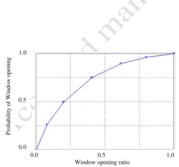
Table 1). The lookups in Figures 4 and 5 show the ‘probability of putting on clothing’ and 195

‘probability of window opening’ based on the qualitative data collected at the model 196

conceptualization stage, details of the data collection for this stage can be found elsewhere, 197

Oladokun (2014). Examples of the developed SD equations are shown in equation 3:5 for the 198

(10)

- 10 - determines the level of occupants’ comfort as a key variable to find the overall carbon 200

emissions as will be discussed next. 201

202

Insert Figure 2 203

Insert Figure 3 204

Insert Table 1 205

Insert Figure 4 206

Insert Figure 5 207

208

OC (t) = INTEGRAL [PDIT, OC (t0)]………(Eq. 1)

209

OMB (t) = INTEGRAL [OAL + PDIT, OMB (t0)]………(Eq. 2)

210

𝐻𝑉 = 𝐼𝐹 (𝐷𝐼𝑇 < 21 ∶ 𝐴𝑁𝐷: 𝑅𝐻 < 45), 𝑇𝐻𝐸𝑁 (𝐷𝐼𝑇), 𝐸𝐿𝑆𝐸 (𝑁𝐷𝐻𝑆) ………..…..…(Eq. 3)

211

𝑁𝐷𝐻𝑆 = 𝐼𝐹 (𝐷𝐼𝑇 < 30 ∶ 𝐴𝑁𝐷: 𝑅𝐻 > 25), 𝑇𝐻𝐸𝑁 (𝑁𝐷𝐻𝑆), 𝐸𝐿𝑆𝐸 (𝑆𝐷𝐻𝑆)……..…...(Eq. 4)

212

𝑆𝐷𝐻𝑆 = 𝐼𝐹 (𝐷𝐼𝑇 < 36 ∶ 𝑂𝑅 ∶ 𝑅𝐻 > 50), 𝑇𝐻𝐸𝑁(𝑆𝐷), 𝐸𝐿𝑆𝐸(𝐺𝐷) ………..…..(Eq. 5)

213 214

Household Carbon Emissions Module 215

The household carbon emissions module simulates end uses of energy, namely; (hot water, 216

space heating, lighting, cooking, and appliances). The developed SFD for ‘space heating’, as 217

an example, is shown in Figure 6. The Figure illustrates the interrelationships among few key 218

variables simulated to calculate the amount of space heating. In addition to ‘Occupants’ 219

behavior’, there are: rate of space heating, space heating energy, effect of energy efficiency 220

on space heating, effect of energy bills on energy consumption, setpoint temp, dwelling 221

internal temp, Space Heating Energy Consumption, energy to carbon conversion, and energy 222

to carbon conversion factor. As indicated by the SD equations (6:10), adding these end uses 223

(11)

- 11 - energy consumption’. Multiplying ‘households’ by this ‘average annual energy consumption 225

per household’ results in the calculation of the total annual household energy consumption. 226

Table 2 shows the data driving this module. The conversion factor ‘energy to carbon 227

conversion’ is then used to determine carbon emissions. For the developed model, this factor 228

is assumed for the conversion of energy from electricity source only. Ideally, a factor for each 229

different fuel source should be identified separately then aggregated for all end uses of 230

energy. 231

232

Insert Table 2 233

Insert Figure 6 234

235

RSH = (SHE * EEESH / EEBEC *1.14 - 0.15 * FORECAST(SHE * 0.53, 39, 450)) * 236

(0.60*ST) / DIT)………. (Eq. 6) 237

SHEC(t) = INTEGRAL [(RSH - ECC), ISHE (t0)]………...(Eq. 7)

238

ECC = SHEC * ECCF………...(Eq. 8) 239

AAECH = CEC + HWEC + LEC + SHEC + AEC………..(Eq. 9) 240

TAHEC = AAECH * HO / 10^6……….(Eq. 10) 241

242

The model uses the three behavioral classifications: ‘frugal’, ‘standard’, and ‘profligate’; 243

adopted from ESRU (2012) and Azar and Menassa (2012). An assumption was informed to 244

formulate the algorithm for energy consumption relative to the frugal, standard, and 245

profligate behaviors based on the data published in the Intertek (2012) report. Further work is 246

underway to consider more occupants’ behavior variables such as: “occupants’ social class 247

(12)

- 12 - variables for this model. External environment variables such as energy securities and 249

political uncertainties are also considered exogenously variables at this stage of the research. 250

251

Behavior Analysis of Occupants Thermal Comfort Module 252

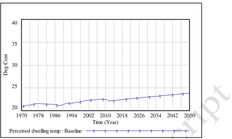
A baseline scenario has been designed to run the proposed model assuming that the existing 253

trends of energy consumption are continuing until 2050. The ‘standard’ occupant’s behavior 254

is assumed for the ‘baseline’ scenario. The dwelling internal temperature is assumed to be 255

19ºC as an average degree for the whole dwelling. 256

257

The perceived dwelling temperature as a model of occupants’ comfort will be the output of 258

this module. However, the input data includes the average relative humidity and the average 259

dwelling internal temperature. The perceived dwelling temperature as produced by the model 260

in Figure 7 is determined based on the Humidex chart in Figure 3. It is clear that the 261

increased pattern of the perceived dwelling temperature resembles the pattern of the average 262

dwelling internal temperature. To obtain better comfort level, the model assumes two 263

occupants’ actions to respond to this increase of the perceived dwelling temperature: putting 264

on higher thermal resistance clothes or opening windows. Relevant qualitative data was 265

collected to model the probabilities of these two actions. As shown in Figure 8, the model 266

results indicate that the probability of putting on higher thermal resistance clothes declines 267

over the years, while the probability of occupants opening windows increases as the 268

perceived dwelling temperature increases. This is consistent with the global climate warming 269

predictions. 270

271

As the perceived dwelling temperature increases, the pattern of occupants’ comfort and 272

(13)

- 13 - a decline in the quest for hot water usage and more space heating is expected. Logically, 274

these growths would reach a saturation level considering the two aforementioned actions of 275

occupants to regulate comfort. Artificial ventilation may be possibly used more if the two 276

occupants’ actions fail to achieve a satisfactory comfort level. 277

278

Insert Figure 7 279

Insert Figure 8 280

Insert Figure 9 281

Insert Figure 10 282

283

Behavior Analysis of Household Carbon Emissions Module 284

The output of the Occupants Thermal Comfort Module is a key input to this module. For the 285

example given in this paper of space heating as one of the components of Household carbon 286

emissions, the behavior of this module will be discussed. 287

288

Figure 11 shows the model results of 15MWh as an average space heating per household for 289

the first four decades. An increase in space heating energy has been observed until 2004, and 290

then a decline is observed. The initial growth is possibly because occupants raise the internal 291

temperature to get better thermal comfort. In 2010, the bad weather conditions led to another 292

sharp increase. As the results show, the space heating energy will continue to decline until 293

2050 mainly because of the energy efficiency improvements in order to comply with building 294

regulations. This decline can be also linked to the increasing energy costs from 2004 as noted 295

by Summerfield et al. (2010) and the milder winters (Palmer & Cooper, 2012). 296

(14)

- 14 - Table 3 illustrates the expected decrease in household carbon emissions in years 2020 and 298

2050 compared with the year 1990 emissions. It is expected that there will be a reduction of 299

49.73 million tones of CO2 by the year 2020 (about 29%). Therefore, based on the assumed

300

‘baseline’ scenario, the reduction of 34% targeted by the 2008 Climate Change Act will not 301

be achieved. For the year 2050, the model results show a reduction of 83.73 million tones of 302

CO2 (about 48%) which also suggests that the conditions of the ‘baseline’ scenario are not

303

sufficient to achieve the reductions of 80% targeted by the 2008 Climate Change Act. 304

305

Having discussed the model results for the baseline scenario, the following section discusses 306

a scenario of occupants’ behavior change over time due to potential more concern about 307

carbon emissions reduction. 308

309

‘Behavioral Change’ Scenario 310

As the major assumptions of the ‘baseline’ scenario are not sufficient to achieve the UK 311

target reduction in carbon emissions, further proposals should be considered. For the 312

developed model, occupants’ behavioural change is assumed as more concern from occupants 313

towards energy consumption is expected. Therefore, ‘frugal’ behaviour is assumed rather 314

than the ‘standard’ behaviour; i.e. attitude of more energy saving. This may make occupants 315

maintain a reduced internal temperature. The dwelling internal temperature is therefore set at 316

18.5ºC. With the ongoing increase in energy prices, energy bills will be assumed higher by 317

5% over the ‘baseline’ scenario values. The household energy efficiency is assumed similar 318

to the ‘baseline’ scenario. The same effects of the ‘average household size’ and the ‘number 319

of households’ are also anticipated as generated by the model based on the historical record. 320

(15)

- 15 - Analysis of the results of the ‘Behavioral Change’ Scenario

322

The total household carbon emission is shown in Figure 12 for the behavioral change effect 323

in comparison with the baseline scenario. Table 3 shows the household carbon emissions in 324

2020 and 2050 compared with the year 1990. The analysis reveals that there is substantial 325

reduction in the energy consumption under the ’behavior change’ scenario which emphasizes 326

Janda’s (2011) comment ‘buildings don’t use energy; people do’. A total of 40.95% and 327

58.47% reduction in carbon emissions relative to 1990 base is expected by this behavioral 328

change by the year 2020 and 2050 respectively. This is actually a decent percentage showing 329

the high impact on energy consumption by occupants’ behavior even without the effect of 330

more advanced energy efficiency improvements. With the effect of more energy efficient 331

technologies installed in dwellings, the target of 80% reduction may be achieved. 332

333

Insert Table 3 336

337

Model evaluation 338

SD models should be first qualitatively evaluated by experts in the field. Sterman (2000) 339

highlighted that model structure should be consistent with relevant descriptive knowledge of 340

the system and conforms to basic physical laws. The level of aggregation of the model should 341

be also appropriate. 342

343

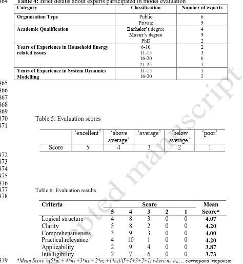
Fifteen experts from energy and SD backgrounds took part in the model evaluation process; 344

brief details about them are shown in Table 4. The interviewees of each field have an average 345

(16)

- 16 - dynamics respectively. The interview started with a description of the research, its aim, 347

objectives, and the purpose of the evaluation process. The interviewees were then given the 348

final CLDs and the SFDs together with the assumptions made for each module. The 349

‘baseline’ scenario and other trial scenarios (including the ‘behavior change’ scenario) were 350

then simulated and the main outputs from the model were presented. Furthermore, the system 351

dynamics experts have had additional scrutiny to test the model behavior, structure, and 352

equations and assess their appropriateness and conformity with the general rules of SD 353

modeling. 354

355

Insert Table 4 356

357

Martis (2006) suggest that models should be adequately evaluated against the criteria of: 358

logical structure, clarity, comprehensiveness, practical relevance, applicability, and 359

intelligibility. A scoring scale attributed for evaluating the criteria is shown in Table 5 and the 360

evaluation results are shown in Table 6. 361

362

Insert Table 5 363

Insert Table 6 364

365

The logical structure assesses the model consistency with the properties of the real system. 366

The mean score of 4.07 (which is above average) indicates that the model has an acceptable 367

logical structure to mimic the real system. The respondents also agree that the model has 368

enough clarity and practical relevance on issues relating to energy consumption and carbon 369

emissions with a mean score of 4.2 for both criteria. A mean score of 4.00 was given to the 370

(17)

- 17 - influence energy and carbon emissions and is capable to address the problem under study. 372

With the assumptions made for the current version of this model, a mean score of 3.87 and 373

3.73 were given to Applicability and intelligibility of the model. While they are still above 374

average, the relatively low scores can be improved by further development of the model to 375

deal with these assumptions. This was clearly addressed in the feedback through highlighting 376

few exogenous variables to be considered endogenous, and through expanding the model 377

boundary to include other excluded variables. Their feedback was recorded for further data 378

collection and modeling. 379

380

The evaluation also aims to validate the SD model by conducting a number of structure-381

oriented tests (e.g. dimensional consistency, parameter assessment, boundary adequacy, 382

structure assessment, integration error, and extreme conditions). There are also a number of 383

behavior pattern tests (e.g. family member, surprise behavior, behavior reproduction, 384

behavior anomaly, system improvement, and sensitivity analysis). Sterman (2000) concluded 385

that a model is behaviorally validated if its results show similarity with the behavior patterns 386

of the real system. Due to space limitation, one test of each group will be presented in this 387

paper. The full details of model evaluation can be found elsewhere; Oladokun (2014). 388

389

Among the main evaluation tests, there is the ‘extreme conditions test’ which evaluates how 390

the model responds to the variation of variables values. The model was run under the extreme 391

values of few key variables. For example, the variables of ‘insulation factor’ and ‘% 392

increment of energy bills’ were selected to show the sensitivity of the model. The two 393

variables are varied between 0% and 100%. Figure 13 and Figure 14 show the model results 394

that indicate the model behavior still make sense without any plausible or irrational response 395

(18)

- 18 - 397

400

The behavior anomaly test is a main test that evaluates how implausible behavior arises 401

should the assumptions made in the model altered, Sterman (2000). In order to conduct this 402

test, a loop knockout analysis was carried out on one of the loops in the occupants’ thermal 403

comfort module to test its effect on the model output. Figure 15 shows the results of the test 404

which indicates that no anomaly or erratic behavior was noticed when the simulation was 405

performed. 406

408

Conclusions 409

A dynamic model is introduced in this paper to simulate occupants’ behavior effects to 410

reduce carbon emissions in dwellings. The systems theory has been followed for the model 411

development to consider the interrelationships among the technical, occupants’ behavior and 412

the external environment of buildings. A number of factors have been used to represent 413

occupants’ behavior based on: Humidex value for different degrees of comfort, the 414

‘probability of putting on clothing’ and the ‘probability of window opening’ within the 415

dwelling, and occupants metabolic build-up. Further work is underway to consider other 416

occupants’ behavior variables such as: “occupants’ social class influence” and “occupants’ 417

cultural influence” which are currently assumed exogenously variables for this model. 418

Furthermore as a limitation to this proposed model, external environment variables such as 419

energy securities and political uncertainties are also considered exogenously variables at this 420

(19)

- 19 - dwelling types on the model results and also the situation of having different temperature 422

degrees within the dwelling units instead of the assumption of one average degree for the 423

whole dwelling. The model can test the effectiveness of certain energy efficient scenarios for 424

the changes in occupants’ behavior. It is concluded that carbon emissions can be vastly 425

reduced by changing occupants’ behavior even without the installation of more energy 426

efficient improvements. With the effect of more energy efficient technologies installed in 427

dwellings, the target of 80% reduction set by the UK Climate Change act 2008 can be 428

achieved. 429

430

Notation 431

The following symbols are used in this paper: 432

433

AEC = Appliances Energy Consumption; 434

AAECH = Average Annual Energy Consumption per Household; 435

CCF = Carbon Conversion Factor; 436

CEC = Cooking Energy Consumption; 437

DIT = Dwelling Internal Temperature; 438

EEBEC = Effect of Energy Bills on Energy Consumption; 439

EEESH = Effect of Energy Efficiency on Space Heating; 440

ECC = Energy to Carbon Conversion; 441

ECCF = Energy to Carbon Conversion Factor; 442

GD = Great Discomfort; 443

HWEC = Hot Water Energy Consumption; 444

HO = Households; 445

(20)

- 20 - ISHE = Initial Space Heating Energy;

447

LEC = Lighting Energy Consumption; 448

NDHS = No Discomfort from Heat Stress; 449

OAL = Occupants Activity Level; 450

OC = Occupants Comfort; 451

OMB = Occupants Metabolic Build-up; 452

PDIT = Perceived Dwelling Internal Temperature; 453

RSH = Rate of Space Heating; 454

RH = Relative Humidity; 455

ST = Setpoint Temp; 456

SD = Some Discomfort; 457

SDHS = Some Discomfort from Heat Stress; 458

SHE = Space Heating Energy; 459

SHEC = Space Heating Energy Consumption; 460

TAHEC = Total Annual Household Energy Consumption. 461

462

References 463

Abrahamse, W., and Steg, L. (2011). Factors related to household energy use and intention to 464

reduce it: the role of psychological and socio-demographic variables, Human Ecology 465

Review, 18 (1), 30-40. 466

467

Accenture. (2010). “Understanding consumer preferences in energy efficiency.” 468

http://www.accenture.com/SiteCollectionDocuments/PDF/ 469

Understanding_Consumer_Preferences_Energy_Efficiency_10-0229_ Mar_11.pdf (Jul. 15, 470

(21)

- 21 - 472

Allcott, H. and Mullainathan, S. (2010). Behavior and energy policy. Science, 327(5970), 473

1204-1205 474

475

Azar, E., Menassa, C.C. (2012). Agent-based modeling of occupants and their impact on 476

energy use in commercial buildings. Journal of Computing in Civil Engineering, 26(4), 506-477

518. 478

479

Azar, E., Menassa, C.C. (2014). Framework to evaluate energy-saving potential from 480

occupancy interventions in typical commercial buildings in the US. Journal of Computing in 481

Civil Engineering, 28(1), 63-77. 482

483

Barr, S., and Gilg, A. (2006). Sustainable lifestyles: Framing environmental action in and 484

around the home. [Article]. Geoforum, 37, 906-920. 485

486

Bartiaux, F., and Gram-Hanssen, K. (2005). Socio-political factors influencing household 487

electricity consumption: A comparison between Denmark and Belgium. ECEEE 2005 488

Summer Study – What Works and Who Delivers?, 1313-1325. 489

490

Bin, S., and Dowlatabadi, H. (2005). Consumer lifestyle approach to US energy use and the 491

related CO2 emissions. [Article]. Energy Policy, 33, 197-208. 492

493

Bourgeois, D., Reinhart, C., and Macdonald, I. (2006). Adding advanced behavioral models 494

in whole building energy simulation: a study on the total energy impact of manual and 495

(22)

- 22 - 497

Building Research Establishment (BRE) (2011). The Government’s Standard Assessment 498

Procedure for Energy Rating of Dwellings 2009 edition incorporating RdSAP 2009, Watford, 499

UK. 500

501

Building Services Research Information Association (BSRIA) (2011). Introducing soft 502

landings. Available at http://www.bsria.co.uk, viewed on 18/07/2011. 503

504

Canadian Centre for Occupational Health and Safety, Humidex chart. Available at 505

https://www.ccohs.ca/oshanswers/phys_agents/humidex.html, viewed on 12/03/2013. 506

507

Carrico, A. R. and Riemer, M. (2011). Motivating energy conservation in the workplace: an 508

evaluation of the use of group-level feedback and peer education, J. of Environ. Psychol., 509

31(1), 1-13. 510

511

Chartered Institution of Building Services Engineers (2006a). Comfort. CIBSE Knowledge 512

Series KS6. London. 513

514

Chartered Institution of Building Services Engineers (2006b). Environmental design. CIBSE 515

Guide A. London. 516

517

Chartered Institution of Building Services Engineers (2013). The limits of thermal comfort: 518

avoiding overheating in European buildings (CIBSE TM52). CIBSE, London. 519

(23)

- 23 - Chen, J., Tayor, J. E., and Wei, H. (2012). Modeling building occupant network energy 521

consumption decision-making: The interplay between network structure and conservation. 522

Energy Build., 47(2012), 515-524. 523

524

Dietz, T., Gardner, G.T., Gilligan, J., Stern, P.C., Vandenbergh, M.P. (2009). Household 525

actions can provide a behavioral wedge to rapidly reduce US carbon emissions, Sustainability 526

Science, 106(44), 18452-18456. 527

528

Energy Systems Research Unit (2012). Household energy upgrade manual. Available at 529

http://www.esru.strath.ac.uk/Programs/EEff/index.htm, Accessed 9th May, 2012 530

531

Fanger, O.L. (1970). Thermal comfort: Analysis and applications in environmental 532

engineering, McGraw-Hill. 533

534

Fritsch, R., Kohler, A., Nygard-Ferguson, M., and Scartezzini, J.L. (1990). A stochastic 535

model of user behaviour regarding ventilation, Building and Environment, 25 (2), 173-181. 536

537

Gill, Z. M., Tierney, M. J., Pegg, I. M., and Allan, N. (2010). Low-energy dwellings: the 538

contribution of behaviours to actual performance. BUILDING RESEARCH AND 539

INFORMATION, 38(5), 491-508. 540

541

Gram-Hanssen, K. (2014). New needs for better understanding of household’s energy 542

consumption – behaviour, lifestyle or practices? Architectural, Engineering and Design 543

Management, 10(1-2), 91-107. 544

(24)

- 24 - Haldi, F., and Robinson, D. (2009). Interactions with window openings by office occupants. 546

[doi: 10.1016/j.buildenv.2009.03.025]. Building and Environment, 44(12), 2378-2395. 547

548

Herkel, S., Knapp, U., Pfafferott, J. (2005). A Preliminary Model of User Behaviour 549

Regarding the Manual Control of Windows in Office Buildings, IBPSA 2005. 550

551

Hitchcock, G. (1993). An integrated framework for energy use and behaviour in the domestic 552

sector, Energy and Building, 20, 151-157. 553

554

Humphreys, M.A., Nicol, J.F. (1998). Understanding the Adaptive Approach to Thermal 555

Comfort, ASHRAE Transactions, 104 (1), 991 – 1004. 556

557

Humphreys, M.A., Nicol, J.F., and Tuohy, P. (2008). Modelling window-opening and the use 558

of other building controls, AIVC Conference, Tokyo, Japan. 559

560

Hunt, D., (1979). The Use of Artificial Lighting in Relation to Daylight Levels and 561

Occupancy, Building Environment, 14, 21–33. 562

563

Intertek (2012). Household Electricity Survey: A study of domestic electrical product usage, 564

available at

565

https://www.gov.uk/government/uploads/system/uploads/attachment_data/file/208097/10043 566

_R66141HouseholdElectricitySurveyFinalReportissue4.pdf 567

(25)

- 25 - International Standard Organisation (1994). Moderate thermal environments – Determinants 569

of the PMV and PPD indices and specification of the conditions for thermal comfort. ISO 570

7730. Geneva. 571

572

IPCC (2007). Climate Change 2007: Mitigation. In: B. Metz, O. Davidson, P. Bosch, R. Dave, 573

L. Meyer (Eds.), Contribution of Working Group III to the Fourth Assessment Report of the 574

Intergovernmental Panel on Climate Change, Technical Report, IPCC. 575

576

Janda, K.B. (2011). Buildings don’t use energy: People do. Architectural Science Review, 54, 577

15-22. 578

579

Kabir, E., Mohammadi, A., Mahdavi, A., and Pröglhöf, C. (2007). How do people interact 580

with buildings environmental systems? Building Simulation, 689-95. 581

582

Kelly, S. (2011). Do homes that are more energy efficient consume less energy?: A structural 583

equation model for England’s residential sector, EPRG Working Paper, Electricity Policy 584

Research Group, University of Cambridge. 585

586

Low Carbon Community Challenge Report (2012). Department of Energy and Climate 587

Change (DECC). Available at 588

https://www.gov.uk/government/uploads/system/uploads/attachment_data/file/48458/5788-589

low-carbon-communities-challenge-evaluation-report.pdf [Accessed on May 9, 2012). 590

591

Mahdavi, A., Pröglhöf, C. (2009). User behaviour and energy performance in buildings, 6. 592

(26)

- 26 - 594

Mason, W., A., Conrey, F. R., and Smith, E. R. (2007). Situating social influence processes: 595

dynamic, multidirectional flows of influence within social networks. Pers. Soc. Psychol. Rev., 596

11(3), 279-300. 597

598

McDermott, H., Haslam, R., & Gibb, A. (2010). Occupant interactions with self-closing fire 599

doors in private dwellings. [doi: 10.1016/j.ssci.2010.05.007]. Safety Science, 48(10), 1345-600

1350. 601

602

Met Office (2013). Climate data. Available at www.metoffice.gov.uk 603

604

Moll, H. C., Noorman, K. J., Kok, R., Engström, R., Throne-Holst, H., and Clark, C. (2005). 605

Pursuing more sustainable consumption by analyzing household metabolism in European 606

countries and cities. Journal of Industrial Ecology, 9, 259-275. 607

608

Martis M.S. (2006). Validation of Simulation Based Models: A Theoretical Outlook. The 609

Electronic Journal of Business Research Methods, 4(1), 39-46 610

611

Motawa, I. and Oladokun, M. (2015). A model for the complexity of household energy 612

consumption, Journal of Energy & Buildings, Vol 87, January 2015, 313–323. 613

614

Natarajan, S., Padget, J., and Elliott, L. (2011). Modelling UK domestic energy and carbon 615

emissions: an agent-based approach. Energy and Buildings, 43, 2602-2612. 616

(27)

- 27 - Newsham, G. R., (1994). Manual Control of Window Blinds and Electric Lighting: 618

Implications for Comfort and Energy Consumption, Indoor Environment, 3, 135–44. 619

620

Nicol, F. and Roaf, S. (2005). Post-occupancy evaluation and field studies of thermal confort, 621

Building Research and Information, 33 (4), 338-346. 622

623

Okhovat, H., Amirkhani, A., Pourjafar, M.R., (2009). Investigating the psychological effects 624

of sustainable buildings on human life, Journal of Sustainable Development, 2(3), 57-63. 625

626

Oladokun, M.G. (2014). Dynamic Modelling of the Socio-Technical Systems of Household 627

Energy Consumption and Carbon Emissions, PhD Thesis (2014), Heriot-Watt University, 628

UK. 629

630

Oreszczyn, T. and Lowe, R. (2010). Challenges for energy and buildings research: 631

Objectives, methods and funding mechanisms. Building Research and Information, 38(1), 632

107-122. 633

634

Palmer J. and Cooper I. (2012). United Kingdom housing energy fact file. London, DECC. 635

Available at 636

https://www.gov.uk/government/uploads/system/uploads/attachment_data/file/345141/uk_ho 637

using_fact_file_2013.pdf 638

639 640

Parys,W., Saelens, D., and Hens, H. (2010). The influence of stochastic modelling of window 641

(28)

- 28 - conference on Low Energy and Sustainable Ventilation Technologies for Green Buildings, 643

Seoul, 26-28 Noember, 1-20. 644

645

Peschiera, G. and Taylor, J. E. (2012). The impact of peer network position on electricity 646

consumption in building occupant networks utilising energy feedback systems. Energy 647

Build., 49(2012), 584-590. 648

649

Rijal, H., Tuohy, P., Humphreys, M., Nicol, J., & Samuel, A. (2011). An algorithm to 650

represent occupant use of windows and fans including situation-specific motivations and 651

constraints. Building Simulation, 4(2), 117-134. 652

653

Scottish Environmental Attitudes and Behaviour (SEAB) (2008). The Scottish environmental 654

attitudes and behaviour survey 2008. Available at 655

http://www.scotland.gov.uk/Publications/2009/03/05145056/11 [Accessed 9th May, 2012). 656

657

Soldaat, K. (2006), Interaction between occupants and sustainable building techniques, In 658

ENHR Conference: Housing in an expanding Europe: theory, policy, participation and 659

implementation, Ljubljana, Slovenia, 2-5 July, 1-15. 660

661

Sterman, J. (2000). Business dynamics: Systems thinking and modelling for a complex world, 662

Irwin McGraw-Hill, Boston. 663

664

Stevenson, F. and Rijal, H. B. (2010). Developing occupancy feedback from a prototype to 665

improve housing production, Building Research & Information, 38 (5), pp 549-563. 666

(29)

- 29 - Summerfield, A, et al., (2010). Two models for benchmarking UK domestic delivered 668

energy. Building Research and Information, 38 (1), 12–24. 669

670

Tweed, C., Dixon, D., Hinton, E, Bickerstaff, K. (2014). Thermal comfort practices in the 671

home and their impact on energy consumption. Architectural Engineering and Design 672

Management, 10(1-2), 1-24. 673

674

Verplanken, B. and Wood, W. (2006). Interventions to break and create consumer habits. 675

Public Policy Mark., 25(1), 90-103. 676

677

Williamson, T., Soebarto, V., and Radford, A. (2010). Comfort and energy use in five 678

Australian award-winning houses: regulated, measured and perceived. Building Research & 679

Information, 38(5), 509-529. 680

681

Yun G.Y. and Steemers, K. (2011). Behavioural, physical and socio-economic factors in 682

household cooling energy consumption, Applied Energy, 88, 2191-2200. 683

(30)

[image:30.595.43.550.89.702.2]

- 30 - 693 694 695 696 697 698 699 700 701

Figure 1: Household Energy Consumption modules 702 703 704 705 706 707 708

Figure 2: SFD for occupants thermal comfort module 709

710 711

Stocks represent accumulations Flows represent the changes to stocks Flow rate

Cloud represents either Source/sink of the flow

Occupants Metabolic

Buildup Occupants Comfort

Perceived dwelling temp Occupants

activity level

probability of putting on clothing

probability of window opening relative humidity

no discomfort lookup

window opening lookup

humidex value

no discomfort from heat stress some discomfort

heat stress

some discomfort lookup great discomfort lookup <some discomfort heat stress> <some discomfort heat stress> great discomfort some discomfort no discomfort growth in occupants activity level <Occupants Metabolic Buildup> <dwelling int temp>

dwelling internal temp 0

(31)

- 31 - 712

713

Figure 3: Humidex chart (Source: Canadian Centre for Occupational Health and Safety) 714

715 716 717 718 719 720 721 722

723 724 725 726 727

Figure 4: Window opening lookup 728

729 730 731

1.0

0.0 0.5 1.0 Window opening ratio

P

roba

bil

it

y of W

indow ope

ning

[image:31.595.172.510.71.324.2] [image:31.595.92.443.356.683.2]

(32)

- 32 - 732

733 734 735 736 737 738

Figure 5: Putting on clothing lookup 739

740 741 742 743

744 745

Figure 6: SFD for space heating energy consumption and carbon emissions 746

747 748

Space Heating Energy Consumption

Space Heating Carbon Emissions rate of space heating

energy to carbon conversion

carbon depletion

energy to carbon conversion factor

carbon depletion rate space heating energy

occupants behaviour space heating

demand

initial space heating energy

initial space heating carbon emissions

<Time> <dwelling

internal temp>

<effect of energy efficiency on space

heating energy>

1.0

0.0 0.5 1.0 Ratio of putting on clothing

P

roba

bil

it

y of p

utt

in

g on c

lot

hing

[image:32.595.75.508.79.686.2]

(33)

- 33 - 749

750

Figure 7: Perceived dwelling temperature under the ‘baseline’ scenario 751 752 753 754 755 756 757 758

Figure 8: Probabilities of putting on clothing and window opening under the ‘baseline’ 759

scenario 760

*Dmnl – dimensionless. 761 762 40 35 30 25

20 1 1 1 1 1 1

1 1 ₁ 1 1 1 1

1 1

1970 1978 1986 1994 2002 2010 2018 2026 2034 2042 2050

Time (Year)

D

eg C

ent

Perceived dwelling temp : Baseline 1 1 1 1 1 1 1 1 1

0.8 Dmnl 0.6 Dmnl 0.6 Dmnl 0.4 Dmnl 0.4 Dmnl 0.2 Dmnl 2 2 2 2 2 2 2 2 2 2 2 2 2 2 1 ₁ 1 ₁ 1 ₁ 1 ₁ 1 ₁ 1 ₁ 1 ₁

1970 1978 1986 1994 2002 2010 2018 2026 2034 2042 2050 Time (Year)

probability of putting on clothing : Baseline 1 1 1 1 1 1 1 Dmnl probability of window opening : Baseline 2 2 2 2 2 2 2 Dmnl

[image:33.595.131.514.68.297.2] [image:33.595.74.533.125.616.2]

(34)

- 34 - 763

764

Figure 9: Occupants metabolic build-up under the ‘baseline’ scenario 765

766 767 768

769 770 771

Figure 10: Occupants comfort under the ‘baseline’ scenario 772

773 774

4

3

2

1

0

1 1

1 1 1

1

1970 1978 1986 1994 2002 2010 2018 2026 2034 2042 2050 Time (Year)

D

m

nl

Occupants Metabolic Buildup : Baseline 1 1 1 1 1 1 1 1

40

30

20

10

0

1 1

1

1970 1978 1986 1994 2002 2010 2018 2026 2034 2042 2050 Time (Year)

D

m

nl

[image:34.595.100.512.68.633.2] [image:34.595.116.513.70.336.2]

(35)

- 35 - 775

776

Figure 11: Average space heating energy consumption per household 777

778 779 780

[image:35.595.79.518.65.631.2]

781 782

Figure 12: Total annual carbon emissions for the UK housing stock for the baseline and the 783

‘behavioural change’ scenarios 784

785

20

15

10

5

0

1

1 1

1 1 1

1

1 1

1

1 ₁

1970 1978 1986 1994 2002 2010 2018 2026 2034 2042 2050 Time (Year)

M

W

h

Space Heating Energy Consumption : Baseline 1 1 1 1 1 1 1

200

150

100

50

0

2 ₂ 2 2 2 ₂

2

2 2

2 ₂

2 2

1

1 1

1 1 1 1

1

1 1

1

1970 1978 1986 1994 2002 2010 2018 2026 2034 2042 2050

M

il

li

on

t

on

ne

s

[image:35.595.144.510.70.287.2]

(36)

- 36 - 786

[image:36.595.103.511.73.334.2]

787

Figure 13: Total annual household energy consumption under ‘insulation factor’ set to 0% and 100%

788 789 790 791 792 793 794

Figure 14: Total annual household energy consumption under ‘increment in energy bills’ set to 0%

795 and 100% 796 797 798 600 450 300 150 0 2 2 2 2 2

2 2 2

2 2 ₂ 2 ₂ 2 ₂ 1 1 1 1 1 1 1 1 1 1 1 1 1 1 1

1970 1978 1986 1994 2002 2010 2018 2026 2034 2042 2050

Time (Year)

T

W

h

total annual household energy consumption : Insulation factor set to 0% 1 1 1 1 1 1 1

total annual household energy consumption : Insulation factor set to 100% 2 2 2 2 2 2 2

600 500 400 300 200 2 2 2 2 2 2 2 2 2 2 2 2 2 2 2 1 1 1 1 1 1 1 1 1 1 1 1 1 1 1

1970 1978 1986 1994 2002 2010 2018 2026 2034 2042 2050 Time (Year)

T

W

h

(37)

- 37 - 799

800 801

Figure 15: Effect of loop knockout on occupants’ thermal comfort module 802

803 804 805 806 807 808 809 810 811 812 813 814 815 816 817 818 819 820 821 822 823 824 825 826 827 828 829 830 831 832 833

40

30

20

10

0

2 2

2

1 1 1

1970 1978 1986 1994 2002 2010 2018 2026 2034 2042 2050

Time (Year)

D

m

nl

Occupants Comfort : Before loop knockout 1 1 1 1 1 1 1

[image:37.595.128.511.68.317.2]

(38)

- 38 - Table 1: Sample data for relative humidity (adapted from: Met Office, 2013)

834 835

Variable Unit of

Measurement

Minimum Maximum Mean Standard Error

Standard Deviation

Relative humidity Percentage 67 94 85.09 1.32 8.67

836 837 838 839 840 841 842 843

Table 2: Sample data for household energy by end-uses (adapted from: Palmer & Cooper, 844

2012) 845

Variable Unit of Measurement

Minimum Maximum Mean Standard Error

Standard Deviation

Space heating MWh 10.14 15.84 13.54 0.18 1.19

Hot water MWh 3.03 6.64 4.78 .17 1.10

Cooking MWh 0.48 1.36 0.86 0.04 0.28

Lighting MWh 0.55 0.69 0.65 0.01 0.04

Appliances MWh 1.07 2.39 1.92 0.06 0.37

846 847 848 849 850 851 852 853

Table 3: The household carbon emissions by end-uses for the baseline and the ‘behavioural 854

change’ scenarios for the year 2020 and 2050 relative to 1990 855

856

(1990) (2020) (2050)

Tonnes of CO2

Baseline Behavioural change Baseline Behavioural change Tonnes

of CO2

*(%) Tonnes of CO2

*(%)

Space heating 94.47 53.19 -43.70 43.76 -53.68 32.46 -65.64 24.35 -74.22 Hot Water 44.15 32.09 -27.32 25.64 -41.93 25.71 -41.77 21.03 -52.37 Cooking 7.93 4.21 -46.91 4.75 -40.10 4.16 -47.54 4.81 -39.34 Lighting 6.04 5.50 -8.94 4.64 -23.18 4.61 -23.68 3.84 -36.42 Appliances 18.43 26.29 +42.65 22.19 20.40 20.35 +10.42 16.99 -7.81

Total 171.01 121.28 -29.08 100.98 -40.95 87.28 -48.96 71.02 -58.47

*Relative to 1990 base as enshrined in Climate Change Act of 2008 857

(39)

[image:39.595.39.513.77.591.2]

- 39 - Table 4: Brief details about experts participated in model evaluation

864

Category Classification Number of experts

Organisation Type Public

Private

6 9

Academic Qualification Bachelor’s degree

Master’s degree PhD