Int. J. Numer. Meth. Fluids2017;00:1–25
Published online in Wiley InterScience (www.interscience.wiley.com). DOI: 10.1002/fld
Multi-dimensional quantification of uncertainty and application to
a turbulent mixing model
Christos Barmparousis
12∗, Dimitris Drikakis
31Fluid Mechanics and Computational Science, Cranfield University, Cranfield, Bedfordshire, MK43 0AL, UK 2CompFlow Computational Engineering, Athens, Greece
3Faculty of Engineering, University of Strathclyde, Glasgow, G1 1XW, UK
SUMMARY
This paper concerns the implementation of the generalized Polynomial Chaos (gPC) approach for parametric studies, including the quantification of uncertainty (UQ), of turbulence modelling. The method is applied to Richtmyer-Meshkov turbulent mixing. TheK−Lturbulence model has been chosen as a prototypical example and parametric studies have been performed to examine the effects of closure coefficients and initial conditions on the flow results. It is shown that the proposed method can be used to obtain a relation between the uncertain inputs and the monitored flow quantities, thus efficiently performing parametric studies. It allows the simultaneous calibration and quantification of uncertainty in an efficient numerical framework. Copyright c2017 John Wiley & Sons, Ltd.
Received . . .
KEY WORDS: Uncertainty Quantification, Turbulence modelling, Meta-model, Calibration, Optimisa-tion, Compressible flows, Polynomial Chaos
∗Correspondence to: Fluid Mechanics and Computational Science, Cranfield University, Cranfield, Bedfordshire, MK43
1. INTRODUCTION
Meta-model methods aim at capturing and representing the behaviour of a random process allowing parametric studies such as sensitivity analysis, optimization and uncertainty quantification to be performed. This is often accomplished by capturing the response of a system to a set of random input parameters. Meta-models are not problem specific and can be used in a wide range of stochastic problems.
Several methodologies have been developed for quantifying the uncertainty in a random process [1]. The UQ methodologies can be divided into probabilistic and non probabilistic. Furthermore, the methodologies can be divided into intrusive [2,3,4,5,6] and non-intrusive [7,8,9,10,11]. Intrusive methods require the modification of the computer codes, while non-intrusive methods consider the computer codes as a ’black box’. In the intrusive framework, the polynomial chaos theory is used to modify the deterministic solver. The modifications of the code can be extensive and complex, therefore only few applications of the intrusive approach can be found in the literature. Despite the complexity in its implementation, the intrusive approach can potentially offer increased computational efficiency as well as accuracy because it allows the uncertainty estimation along with the solution. The deterministic code has to run only once but it may involve long computing times that depend on the order and dimension of the uncertainty imposed. A drawback of this approach is that geometrical uncertainties are difficult to be taken into account due to numerical implementation issues.
For the non-intrusive approach several calculations using the deterministic code need to be performed depending on the number of uncertain inputs and degree of accuracy required. A direct comparison of intrusive and non-intrusive methods is not straightforward. Under certain conditions, the non-intrusive approach can also be accelerated and be computationally efficient as the intrusive approach.
In the non-probabilistic approach the result of the uncertainty is presented in a form which does not include information about the likelihood or the probability distribution of the measured quantity [12]. In general, these methods are easier and faster to implement but they can only estimate the minimum and maximum value of the monitoring quantity. The major drawback is that no confidence interval or any other high-order statistics can be obtained. On the other hand, the probabilistic approaches are more complicated but they provide far more detailed information about the variation of the monitoring quantity with respect to the random inputs.
spanned by a set of complete orthogonal polynomials. The rate of convergence of a PC expansion is strongly related to the level of correlation.
A modified version of PC was proposed by Xiu and Karniadakis [14], known as generalized Polynomial Chaos (gPC) or Wiener- Askey (WA) scheme since it is based on the family of polynomials found in the Askey scheme [15]. The gPC results in a more efficient representation of the stochastic process when the process follows a known probability distribution. However, this is not often the case, therefore the probability distribution should be defined at the input level. The type of input distribution is represented by a weight function in the polynomials of the expansion basis. This generalized framework combined with the multi-index notation provides a very flexible method to represent a random process that has inputs that follow different probability laws. The generalized PC extends the convergence properties of the classical PC since the polynomials are originated from the Askey scheme [16]. Through the gPC, it is possible to represent a multi-dimensional stochastic model with inputs that have different probability distribution functions. In addition to the extended polynomial families, the random inputs can also be represented through a discrete type of distributions, a convenient option for cases where the random input is expressed by discrete samples. If the optimal expansion base is selected, exponential error convergence is achieved as per the basic PC. In cases where the optimal basis is not selected, the convergence is also guaranteed but not at an exponential rate. Past publications have dealt with the numerical properties of gPC [17] and its application to engineering problems[4,18,19] and CFD simulations[20,21]. Application of gPC to engineering turbulence modelling (TM) is scarce [22,23,24,25]. In its intrusive form, the method presents a number of challenges when applying it to turbulent flows [26,27,28,29]. One of the main motivations behind the use of the non-intrusive form is its ability to converge, although not in the mean square sense, even when the response function is not known in advance. This allows the method to be executed in independent runs fully utilising the black box approach through decoupled parallel runs. This is in contrary to other methods that are strongly coupled with the response function. In practise this significantly increases the implementation flexibility of the method.
TM of shock-induced turbulent mixing associated with hydrodynamic instabilities, such as Rayleigh-Taylor (RT), Richtmyer-Meshkov (RM) and Kelvin-Helmholtz (KH), encompasses several challenges. In addition to the shock waves and material discontinuities, turbulent mixing features baroclinic effects due to variable-density and vorticity production at material interfaces, as well as anisotropy and inhomogeneity resulting from initial and boundary conditions.
modelling assumptions and closure coefficients are validated and calibrated, respectively, by comparisons with experiments but even more commonly through high-resolution large eddy (LES) and direct numerical simulations (DNS).
The simplest type of model uses ordinary differential equations for the width of the RT/RM mixing layer, where the bubble or spike amplitudes are described by balancing inertia, buoyancy and drag forces; these are called buoyancy drag models[33,34,35,36]. These models are of limited use as they cannot model multiple mixing interfaces; cannot be easily extended to two and three dimensions; and cannot model de-mixing. To address these problems, a second category of models has been proposed, the so-called two-fluid (or multi-fluid models) [37,38,39,40,41]. These models use one set of equations for each fluid in addition to mean flow equations. The models are fairly complex but provide an accurate modelling framework for de-mixing and capturing correctly the relative motion of the different fluid fragments. Finally, an intermediate class of models maintains the individual species fraction but assigns a single fluctuation velocity for the mixture. The models are also known as two-equation turbulence models because they consist of evolutionary equations for the turbulent kinetic energy per unit mass and its dissipation rate or the equivalent turbulent length scale [42, 43, 44]. These models postulate a turbulent viscosity, a Reynolds stress, and dissipation terms as well as a buoyancy term for modelling RT and RM instabilities. They are able to handle multi-dimensions, multi-fluids, and variable accelerations, however, they cannot capture (in their present form) the de-mixing process. A more advanced version of the single fluid approach is the BHR (Besnard-Harlow-Rauenzahn) model, which has evolved over the years [45,46]. The aim of this study is to demonstrate the application of the gPC approach in conjunction with an existing turbulence model. The study does not aim to provide an assessment of the accuracy of the K−Lmodel for compressible turbulent mixing or investigate the physics of compressible turbulent mixing. A comprehensive study on the accuracy of theK−Lmodel has recently been presented in [47]. The model is popular within the inertial confinement fusion (ICF) community and has extensively been used in ICF predictions; see [42,47,48] and references therein.
Figure 1. Schematic of the RMI instability growth
2. TURBULENCE MODELLING
RMI occurs as a result of an impulsive acceleration at the interface of two fluids of different densities, e.g., when a shock wave passes through an interface separating two fluids. An uneven fluid interface or surface roughness usually creates the perturbed interface. The development of the instability is due to the misalignment of the pressure gradient with the local density gradient and grows self-similarly at early times. It grows forming spikes (S) and bubbles (B) that penetrate the light and heavy fluid with different growth rates (hs and hb Figure1). At late times, it becomes
highly non-linear, thus leading to turbulence and turbulent mixing.
The amplitude of the perturbation has an effect on the initial growth rate of the instability with low amplitudes leading to linear growth. A single characteristic (narrowband) perturbation will grow following a power law that has an exponent of the order θb≈0.26, while the broadband is
more likely to exhibit an exponent ofθb≈2/3:
hb∝tθb (1)
In addition, it has been shown that the growth rate is also correlated to the density ratio of the two fluids[35]. The mixing occurs at high Reynolds number [32,49], therefore the flow characteristics can be obtained assuming that the viscosity of the fluid is insignificant without any great loss of accuracy. The spike and bubble position are identified by the mass fraction level, which in the present work are 0.01 and 0.99, respectively. The volumetric fraction is given by
fi= F ri Mi F r1
M1 +
F r2
M2
(2)
whereM is the molecular weight andF ris the mass fraction. Additional key parameters frequently investigated are the Integral Length of Mixing Zone (ILMZ) and the Total Mix (TM):
ILM Z =
ˆ L
0
hf1i · hf2idx (3)
T otalM IX =
ˆ L
0
ρ1·F r1·ρ2(1−F r2)dx (4)
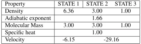
Property STATE 1 STATE 2 STATE 3
Density 6.36 3.00 1.00
Adiabatic exponent 1.66
Molecular Mass 3.00 3.00 1.00
Specific heat 1.00
[image:6.595.174.419.66.142.2]Velocity -6.15 -29.16
Table I. Fluid properties of the single planar case initialization.
g=1 ρ
∂P
∂x (5)
Ao≡
(ρ2−ρ1)
(ρ2+ρ1)
(6)
whereρ1andρ2are the densities of the two fluids. In the case of an impulsive acceleration (RM
instability, the bubble growth is described by the power law:
hb∝(Uint·t)θb (7)
where the Uint is the velocity due to the shock passage at the interface between the two fluids
and θb∼0.4(2D),0.25±0.05(3D)is the bubble exponent. The impulsive acceleration is usually
achieved through the passage of a shock wave (Richtmyer Meshkov instability).
Similar to [42], a one-dimensional domain is used (x-direction) with the shock wave moving towards the positive direction. The post shock Atwood number used in the present simulations is kept constant at A+≈0.5. The perturbed interface is placed after the shock and the initialization
of theK−Lmodel is applied on two cells around the interface. The domain outside the perturbed cells is initialized with(K0, L0= 0).
In the framework of turbulence modelling for RMI, the governing equations can be reduced to their one dimensional counterpart. Dimonte and Tipton [42] proposed a two-equation model using the the turbulent kinetic energyKand the characteristic length scaleL. This modelling approach assumes a single velocity component for both fluids and has been applied successfully to one dimensional problems [50]. The equation forLdescribes the average size of the characteristic length scale of both spike and bubble. The growth ofLis self similar and is directly proportional to the initial perturbationL∝h0. The diffusion ofLis scaled by a relevant scaling coefficientNL. The
equation includes the compressibility effects and energy exchange. The proposed equation for the evolution of the average characteristic length scale is given by
¯ ρDL
Dt = ∂ ∂x
µT
NL
∂L ∂x
+ρV +CCρL¯
∂u˜
∂x (8)
The proposed equation for the evolution of the turbulent kinetic energy is given by
¯ ρDK
Dt = ∂ ∂x
µ
T
NK
∂K ∂x
+SK (9)
Dρ
Dt = −ρ ∂u˜
∂x (10)
¯ ρD
˜ Fr
Dt = ∂ ∂x
µT
NF
˜ ∂Fr
∂x
(11)
¯ ρDu˜
Dt = − ∂P
∂x − ∂τj
∂x (12)
¯ ρD˜
Dt = ∂ ∂x
µT
N
∂˜ ∂x
−P∂u˜
∂x −SK (13)
where all the bar-quantities are Favre-averaged;µT is the turbulent eddy viscosity;NandNF are
model coefficients.SKis a source term extracting energy from the mean flow and its formulation is
based on the buoyancy-drag model:
SK = ¯ρ·V ·
CB·A·g−CD
V2
L
(14)
whereCB andCDare coefficients.V is given byV =
√
2Kand the eddy viscosity is modelled as
µT ≡CµρLV¯ (15)
Cµ is a finite unknown value whose estimation is mostly influenced by the KH instability. Its
calibration is compromised by velocity limiters used to constrain unphysical strain rates. Due to the absence of a realisable turbulent shear stress term the model cannot model KH instability growth reliably. This deficit is somehow compensated by settingCµ= 1The Atwood number described in
equation (6) has been modified in order to reproduce the quantities modelled as well as to account for the flow discontinuities. The deviatoric tensor in the momentum equation is modelled by:
τij=Cp·δij·ρ·K , (16)
where the coefficientCpis correlated with the Mach number which is corrected to take into account
the absence of realisable turbulent shear stress. The Atwood number proposed for the K-L model is:
Ai ≡
¯ ρr−ρ¯l
¯ ρr+ ¯ρl
+CA
L ¯
ρ+L|∂ρ/∂x¯ |
∂ρ¯
∂x (17)
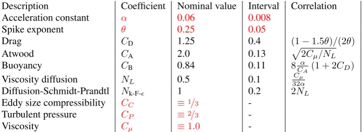
Description Coefficient Nominal value Interval Correlation
Acceleration constant α 0.06 0.008
Spike exponent θ 0.25 0.05
Drag CD 1.25 0.4 (1−1.5θ)/(2θ)
Atwood CA 2.0 0.13
p
2Cµ/NL
Buoyancy CB 0.84 0.11 8CAα (1 + 2CD)
Viscosity diffusion NL 0.5 0.1 32Cµα
Diffusion-Schmidt-Prandtl Nk-F- 1 0.2 2NL
Eddy size compressibility CC ≡1/3
-Turbulent pressure CP ≡2/3
-Viscosity Cµ ≡1.0
-Table II. K−Lnominal closure coefficients and their corresponding interval calculated from the relevant correlation formula.
The K-L model has been numerically implemented for the compressible Euler equations (molecular effects assumed negligible) using the finite volume Godunov-type [56] (upwind) method. Additionally, the following is used: 1) the isobaric assumption to estimate the heat capacity ratio of the mixture equation (2); 2) the MUSCL 5th-order [57] augmented by a low Mach number
correction [?] for reconstructing the variables [ρ(1−F), ρu, p, ρF, ρK, ρL]; 3) the HLLC solver [52] along with the pressure-based wave speed estimate (PVRS) method for the solution of the numerical inter-cell flux estimation (Riemann problem); and 4) a third order TVD Runge-Kutta scheme for time integration; see [58, 59] and references therein. It has been found that the above procedure does not generate any unphysical pressure oscillations at the interface between components of different heat capacity ratios (γ16=γ2).
3. SOURCES OF UNCERTAINTY
There are two major sources of uncertainty in the K−L model: (i) the initial conditions at the perturbed interface; and (ii) the coefficients, which are usually fitted to experimental data and also varied to match different flow configurations thus presenting both aleatoric and epistemic type of uncertainties. The uncertainties associated with the initial conditions are attributed to the difficulty in controlling the surface of the perturbed interface which classifies them as aleatoric uncertainties. The above sources of uncertainty will be investigated in two independent studies. The nominal values of the coefficients used byK−Lmodel are listed in TableII.
The coefficients are classified into dependent and independent, which reduces the actual number of uncertain parameters to two : θ and α. The dependent coefficients (CD,CA,CB, NL, Nk-F-)
varied following their correlation formula while the remaining independent coefficients (CC,CP,
Cµ) were kept constant for every numerical investigation. The nature of the two uncertain parameters
is described in the following subsections.
The dimensional analysis used to formulate the turbulence model does not take into account the fact that a number of bubbles grow twice as fast compared to a bubble with a similar characteristic length [60, 61, 62, 63]. For low Atwood numbers (A <0.05) the variation is small [64, 65]
[image:8.595.115.485.66.201.2]the corresponding spike exponent can be significantly different and this simplification used in the turbulence model can be another source of uncertainty. A number of numerical simulations have been performed in an attempt to estimate the variation ofα[35,67]. The experimental procedures can vary between different experiments and this is considered as an additional source of uncertainty. The investigation has been performed by allowingαto vary between0.052and0.068.
Once the flow becomes self-similar the growth of the instability is described by the power law and the corresponding coefficientθ. Numerical and experimental investigations suggested slightly different values forθ[68,35,69,35,66,70,33]. The discrepancies in the estimation between the experiments and the numerical simulations are mainly due to the different perturbation wavelengths [71]. Furthermore, the power law coefficient is correlated with the density ratio of the two fluids. The above suggest thatθcannot be universal, however, in theK−Lmodel a universal exponent is used instead, thus resulting in an additional source of uncertainty. According to the original formulation of the model, the value ofθhas been varied in the range of0.2< θ <0.3.
The dependence of the growth rate on the initial conditions has been investigated in [32]. The uncertainty arises from the difficulty to precisely control the perturbed interface as well as to take this into account in the framework of numerical simulations. In high fidelity LES, a two dimensional perturbation, based on a characteristic length scaleη0, is imposed on the interface.
The initialization of K has been obtained using the relation V =√2·K and its self similar evolutionary equation:
dV0
dt =CBA0g⇒V0=CBA0gdt (18) Equation18is derived by9assuming an incompressible flow and by taking into consideration that the buoyancy term inSK is significantly higher compared to the drag term. In reality,K1 should
be equal to zero since no turbulence exists prior to the initiation of the mixing process. This is not practical since every term that includesV will be equal to zero suggesting no change of the turbulent kinetic energy during the simulation. To overcome this and make the evolution ofKindependent of the initial conditions a two-step process is employed. The initialization ofKis obtained by assuming thatVnew≈CB·A·g·δtrepresents the state exactly after the initialization of the flow. TheK1can
then be found using an iterative process to obtain the accelerationg≈2×10⁴/6with a time-step δt= 10−4:
K1=
V2 new−V02
2 ≈0.11 (19)
Due to its dependence onCBand hence onα, the initialization ofKcannot be achieved assuming
a fixed value. Considering the highest level of uncertainty seen in the experimental investigations of α,Kwas assumed to vary in the following interval :0.05< K1<0.15.
An important source of uncertainty is the initial length scaleL1. The interface perturbation can
be correlated to the initial length scale byL1≈η02. This indicates that the width of the initialization
should be approximately equal to the amplitude of the perturbation. According to Dimonte and Tipton, the initialization ofL1att= 0is given by
L1≈
η2 0
In this study, the variation of the initial perturbation has been set to50%, hence0.1< L1<0.3.
4. THE POLYNOMIAL CHAOS
The original formulation of polynomial chaos was the first step towards the quantification of a random process whose properties are not known a priori. It is described by Weiner [13] as the theory of homogeneous chaos and is an efficient formulation that can be used to estimate the uncertainty involved in a non-linear stochastic process . The “Homogeneous Chaos” as defined by Weiner provides a formulation for expanding a second-order random process using a set of polynomials based on a centred, normalized Gaussian type of random variables ξi. The polynomial space of
orderpis denoted asΨˆp, while the set of polynomials belonging to this space and order are denoted
as Ψp and are known as the basis functions. The polynomial chaos type of expansion involves
all of the unique combination polynomials at the selected order. The polynomial chaos is a set of functions of the random variablesξ. The distinctive advantage of the PC theory is that it remains valid for any level of correlation and that it converges in the mean square sense. The basic principle of this methodology is to project the variables of the problem onto a stochastic space spanned by a set of complete orthogonal polynomialsΨ. The rate of convergence of a PC expansion is strongly related to the level of correlation.
Using this approach every random process can be expressed using the PC expansion. For example, the finite dimensional representation of a stochastic processU in one dimensional space, which is dependent on a random variableωas well as on independent variablesx, t, can be represented as:
U(x, t, ω) =
∞ X
i=1
ui(x, t)×Ψi(ξ(ω)) (21)
However, in reality, this has to be limited to a finite number of chaotic expansionsM+ 1:
U(x, t, ω) =
M+1 X
i=0
ui(x, t)×Ψi(ω)) where: M+ 1 =
(Npc+p)! Npc!×p!
(22)
In the above equations, the following apply:
• ui(x, t)represents the deterministic coefficients, known as PC coefficients , and are denoted
as the random node (i) of the process.
• The spectral representation of uncertainty is based on the trial basis of a set of complete orthogonal polynomials. It is a function of random variablesξ, which are functions of the random parameterω.
• NP Cis the number of random dimensions andpis the order of expansion.
• There is direct relation between the basis of the expansionΨiand the Hermite polynomials
Hnin the formulation proposed by Wiener.
• The dimension of the system is expressed by the basis functions and their polynomials.
The mean-square convergence indicates that the finite expansion converges aspgoes to infinity:
lim
p→∞E
h
(u0Ψ0+. . .+upΨp−U) 2i
The convergence rate is in accordance with the Cameron-Martin theorem and it has been demonstrated that exponential convergence is achieved when the process is Gaussian. Furthermore, the expansions of orders greater than zero vanishes:
E[Ψp>0] = 0 (24)
It is clear that the PC efficiency is directly related to the number of random variables and the requested order. The method becomes rapidly inefficient as the values of the above parameters increase. The error due to the truncation is also convergent in the mean square sense:
lim
N,p→∞
2(N, p)= 0 (25)
4.1. The estimation of the expansion coefficients
The number of expansion coefficientsM is a function of the uncertain parameters and the desired expansion order (Eq 22). This results in a set of equations equal to the number of the expansion coefficients. For three random parameters (three dimensional uncertainty) the expansions take the following form:
U(0) = u0+ M X
i=1
ui1Ψ1i1(ξ
(1)
i1 ) +
M X i1=1 i1 X i2=1
ui1i2Ψ2i1i2(ξ
(1)
i1 , ξ
(1) i2 ) + M X i1=1 i1 X i2=1 i2 X i3=1
ui1i2i3Ψ2i1i2(ξ
(1)
i1 , ξ
(1)
i2 , ξ
(1)
i3 )
U(1) = u0+ M X
i=1
ui1Ψ1i1(ξ
(2)
i1 ) +
M X i1=1 i1 X i2=1
bi1i2Ψ2i1i2(ξ
(2)
i1 , ξ
(2)
i2 ) (26)
+ M X i1=1 i1 X i2=1 i2 X i3=1
bi1i2i3Ψ2i1i2(ξ
(2)
i1 , ξ
(2)
i2 , ξ
(2)
i3 )
.. .
U(i) = u0+ M X
i=1
ui1Ψ1i1(ξ
(i)
i1) +
M X i1=1 i1 X i2=1
ui1i2Ψ2i1i2(ξ
(i)
i1, ξ
(i)
i2) + M X i1=1 i1 X i2=1 i2 X i3=1
ui1i2i3Ψ2i1i2(ξ
(i)
i1, ξ
(i)
i2, ξ
(i)
i3)
Each code response U(i) corresponds to one of the above equations. In order to calculate the desired coefficients (ui) the above formulas are transformed into a matrix form which can be solved
1 Ψ1(ξ(1)
1 ) · · · Ψ1(ξ (1)
N ) Ψ
2 1(ξ
(1)
1 ) · · · Ψ2K2(ξ
(1)
N ) Ψ
3 1(ξ
(1)
1 ) · · · Ψ3K3(ξ
(1)
N )
1 Ψ1(ξ1(2)) · · · Ψ1(ξN(2)) Ψ21(ξ(2)1 ) · · · Ψ2K
2(ξ
(2)
N ) Ψ
3 1(ξ
(2)
1 ) · · · Ψ 3 K3(ξ
(2)
N )
1 ... ... ... ... ... ... ... ... ...
1 Ψ1(ξ(M)
1 ) · · · Ψ1(ξ (M)
N ) Ψ
2 1(ξ
(M)
1 ) · · · Ψ2K2(ξ
(M)
N ) Ψ
3 1(ξ
(M)
1 ) · · · Ψ3K3(ξ
(M)
N ) × u0 u1 .. . uM = U0 U1 .. . UR (27)
Or in a more compact formAijuj =U(i), i= 1,· · ·M+ 1, j= 1,· · ·M
4.2. The generalized Polynomial chaos
In this work the distribution of the uncertain parameters do not follow the Gaussian profile requiring the use of the generalised polynomial chaos (gPC) An increase in the efficiency for the representation of the stochastic process is achieved in cases where the process in question follows a known probability distribution. In reality this is rarely the case, indicating that the only stage where efficiency increase can be achieved is at the representation of the random input. The type of input distribution has to be reflected by the weight function used in the polynomials of the expansion basis. If the optimal expansion base is selected, exponential error convergence is achieved as per the basic PC. In cases where the optimal basis is not selected convergence is also guaranteed but not at an exponential rate.
Since no specific knowledge on the distribution is known, for this work all the random inputs will be assumed to follow a uniform distribution hence the expansion basis will be the Legendre polynomials:
Ψi(ω) =Lei(ω) =
1 2i
[i/2] X
l=0
(−1)l i l
!
2i−2l n
!
ωi−2l (28)
where[ ]denotes the integral part.
4.3. Algorithmic implementation
The gPC implementation is achieved through the development of a relevant computational code [72] . The code performs symbolic and not numerical operations, a method known to preserve accuracy and computational efficiency [73,74,11,75]. It has been developed following the modular approach verifying each part in a step by step process. In addition to the PC functionality the code was also extended to automate the post processing using the reconstructed response. Each investigation has been performed using a three step process:
1. Sampling process
(b) Generation of quadrature points.
(c) Transformation and normalisation of the random sample sets between the required distributions.
2. Expansion construction
(a) Construction of multidimensional polynomials using the multi index algorithm. (b) Tensor product estimation.
(c) Expansion coefficients estimation through direct matrix inversion.
3. Post processing
(a) Meta model construction using the previously estimated coefficients
(b) Statistical sampling studies using the symbolically reconstructed response (functional approach).
(c) Execution of parametric studies (sensitivity, uncertainty bars and optimisation).
The code has been parallelised to run on shared memory machines. The solution of the system of equations is obtained for the PCM methods using direct solvers. The code is monitoring the stiffness of the system and is able to switch to iterative solvers. The solution of the system is not preconditioned and the conversion from symbolic manipulations to numerical approximations is obtained using fixed point arithmetic methodologies with 25 digits of accuracy. The aforementioned reconstruction process is separately performed for each monitoring point.
5. PARAMETRIC STUDY USING GPC
The sampling of the random parameters (α, θ andK1, L1) has been done at the collocation points
of the expansion basis. The convergence has been monitored through the response shape and the variation of the mean and CI with respect to the expansion order. In most cases, the polynomial expansion converged after the 4th expansion but for consistency an 8th order reconstruction will be used. The responseReifor the ILMZ and Tmix has been logged fori= 30points at an interval of
0.5sstarting at0.5s. The cumulative error is obtained through relevant high fidelity data [32] and normalized at the same monitoring pointsmpin a percentage scale:
Comulative Error=
i=mp X
i=1
ReiKL−ReiILES
ReILES
∗ 100
mp (29)
Coefficient α θ Mean (experimental) 0.06 0.25 Linear Variation (±) 0.008 0.05 Minimum value 0.052 0.2 Maximum Value 0.068 0.3
Table III. Coefficients variation used for the sensitivity analysis
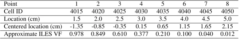
has always been performed using the Monte Carlo method over a set of 500,000 realisations of the reconstructed response and the CI covered 95% of the sample distribution. The monitoring points of the volume fraction (VF) investigations are presented in TableIV.
Point 1 2 3 4 5 6 7 8
Cell ID 4015 4020 4025 4030 4035 4040 4045 4050
Location (cm) 1.5 2.0 2.5 3.0 3.5 4.0 4.5 5.0
Centered location (cm) -1.35 -0.85 -0.35 0.15 0.65 1.15 1.65 2.15 Approximate ILES VF 0.978 0.849 0.610 0.377 0.210 0.100 0.040 0.012
Table IV. Position properties of the selected points for the VF investigation att= 10s.
5.1. Initial conditions
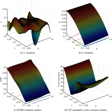
Rapid convergence rate has been observed for most of the initial conditions studies. The investigation with respect toαindicates only small changes in the results (figure2a), which cannot be adequately captured due to the nature of the polynomials as explained by the Runge function theory [76,77]. The relatively small response in the variation magnifies the numerical rounding error of the reconstruction process, which is manifested by the high residual level in the coefficient matrix inversion. The effect of the initial conditions onθhas been captured using second-order (and higher) expansions, as shown in figure2b, while the initial value of the turbulent kinetic energy does not significantly affect the exponent. It has been shown that the initialisation ofLhas the highest influence producing a smooth variation along its interval. An identical response is also observed for the ILMZ case, where the response is weakly correlated with the initial TKE (figure2c). The cumulative error of the volume fraction (figure2d) also indicates that the response is not affected by the uncertainties associated with the initialisation of K. The response minimises its deviation from the reference data at a unique value of initial characteristic length at approximatelyL1≈0.24.
The level of deviation from the reference data increases when increasing L. A lower rate of error increase is observed at the smallest values ofL.
[image:14.595.103.493.245.309.2]0.05
0.1
0.1 0.15 0.2 0.25 0.3
0 0.05 0.1 0.15
K L
α
(a)αvariation
0.05
0.1
0.1 0.15 0.2 0.25 0.3 0.2 0.205 0.21 0.215 0.22 0.225 0.23
K L
θ
(b)θvariation
0.05
0.1
0.1 0.15 0.2 0.25 0.3 0.4 0.45 0.5 0.55 0.6
K L
ILMZ
(c) ILMZ response surface
0.05
0.1
0.1 0.15 0.2 0.25 0.3
28 30 32 34 36 38 40
K L
% VF Com Error
[image:15.595.111.478.75.437.2](d) VF cumulative error response surface
Figure 2. Response plots of the initial conditions study(varying K0−L0).
5.1.1. Atwood number dependence The Atwood number investigation has been performed by
changing the initial conditions for the heavy fluid, while keeping constant the density of the light fluid as ρL= 1g/cm. The initialization ofK has also been adjusted by using equation 18.
Using a 6th-order PCM type of expansion, the stochastic input has been sampled at 7 points. The uncertain parameterρH varied in the interval1.1to9resulting in an Atwood number variation of
0.04< A <0.8. The growth exponentθis estimated by fitting the non-linear bubble equation7to ILMZ, bubble and spike position plots.
0 2 4 6 30
35 40 45 50 55 60 65 70 75
Time (s)
% Variation
ILMZ Total Mix Total TKE
(a) Uncertainty level decay over time.
0 0.2 0.4 0.6 0.8 0.24
0.26 0.28 0.3 0.32 0.34 0.36 0.38
Atwood
θ
ILMZ Bubble Spike
[image:16.595.114.481.76.257.2](b) Growth exponent coefficients variation with respect to the Atwood number
Figure 3. Growth exponent variation and uncertainty decay over time for the initial conditions study.
5.2. Closure coefficients
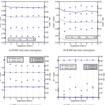
5.2.1. Convergence properties: The ILMZ convergence study shown in figures4aand4bindicates
1 2 3 4 5 6 7 8 0.24 0.26 0.28 0.3 0.32 0.34 0.36 0.38 0.4 0.42
Expansion order p
ILMZ − mean
0.03 0.04 0.05 0.06 0.07 0.08 0.09 0.1 0.11
ILMZ − Std
1s 2s 4s 6s
(a) ILMZ early time convergence
1 2 3 4 5 6 7 8 0.42 0.44 0.46 0.48 0.5 0.52 0.54
Expansion order p
ILMZ − mean
0.09 0.1 0.11 0.12 0.13 0.14 0.15 ILMZ −Std
8s 10s 12s 15s
(b) ILMZ late time convergence
1 2 3 4 5 6 7 8 0 0.2 0.4 0.6 0.8 1
Expansion order p
VF − mean
0 0.01 0.02 0.03 0.04 0.05 0.06 0.07 0.08 0.09
VF − Std
CI point 3 CI point 5 Mean point 3
Mean point 5
(c) VF inner points convergence
1 2 3 4 5 6 7 8 0 0.2 0.4 0.6 0.8 1
Expansion order p
VF − mean
0 0.01 0.02 0.03 0.04 0.05 0.06 0.07 0.08 0.09
VF − Std
CI point 1 CI point 8 Mean point 1
Mean point 8
[image:17.595.117.479.76.437.2](d) VF outer points convergence
Figure 4. Convergence plots of Mean and Standard deviation for the ILMZ and VF profile
5.2.2. Reconstructed response: Good agreement with the ILES data is observed for the prediction
0 2.5 5 7.5 10 12.5 15 0 0.1 0.2 0.3 0.4 0.5 0.6 0.7 Time (Sec) ILMZ 15 20 25 30 35 % Variation
KL + UQ ILES
% Deviation
(a) ILMZ
0 2.5 5 7.5 10 12.5 15 60 80 100 120 140 160 180 200 220 240 260 Time (Sec) Total MIX 15 20 25 30 35 % Variation % Variation
(b) Total Mix
0 2 4 6 8
0 0.01 0.02 0.03 0.04 0.05 Monitoring point TKE PCE
αLθL α
LθH αHθL αHθH
(c) TKE profile at t=2s
0 2 4 6 8
−1 0 1 2 3 4 5 6x 10
−3
Monitoring Point
TKE
PCE αLθL αLθH αHθL αHθH
(d) TKE profile at t=10s
0 2 4 6 8 0 0.2 0.4 0.6 0.8 1 1.2 Monitoring point Volume Fraction 0 20 40 60 80 100
% Variation
KL PCE ILES Low α Low θ High α High θ
% var
[image:18.595.113.481.70.626.2](e) VF profile at t=10s
Figure 5. Error plots due to the uncertain closure coefficients.
highlighted. The highest levels of deviation with respect to the reference data are obtained by the outer values of the recommended interval of the two coefficients; however, the deviation is not symmetric.
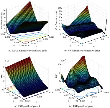
The volume fraction (Figure 6b) response does not follow the characteristics observed for the previous monitoring quantities. More than one region, where the deviation with respect to LES data can be minimized, is detected, while the effect ofθvariation is not as significant as it was for the previous cases.The maximum and minimum magnitude of the TKE profile (Figure 6c) is highly correlated to θ and weekly correlated to α. The two closure coefficients mainly affect the inner region of the profile, which appears to be captured adequately by the reconstruction process. The unphysical values of the outer points (Figure6d) in the reconstructed responses, where negative TKE values are observed, can be attributed to the limitation of the reconstruction process to accurately capture sudden changes of the response.
0.052 0.054
0.060 0.064
0.068
0.200 0.225 0.250 0.275 0.3000
5 10 15 20 25 30
α θ
% Comulative Error
(a) ILMZ normalised cumulative error
−1 −0.5
0 0.5
1
−1 −0.5 0 0.5 1 30 40 50 60 70 80 90 100
α θ
VF % Comulative error
(b) VF normalised cumulative error
0.052
0.054
0.060
0.2 0.225 0.250 0.275 0.3
1 2 3 4 5
x 10−3
α θ
TKE
(c) TKE profile of point 4
0.052
0.054
0.060
0.2 0.225 0.250 0.275 0.300
0 5 10
x 10−4
α θ
TKE
[image:19.595.110.484.271.638.2](d) TKE profile of point 8
Figure 6. Response surfaces.
5.2.3. Sensitivity analysis: Given that the viscosityCµ is defined as a fixed value, the sensitivity
performed for the key flow quantities (ILMZ, otMix and Total TKE ). The selected quantities have been monitored at five time points (1.5, 4.5, 7.5, 10.5 and 15 seconds) in an attempt to get an evenly spaced set of sensitivity results. All the reconstructed responses were of 8th order and were obtained after 45 deterministic code realisations.
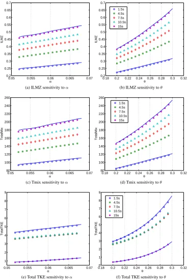
The definition of ILMZ (Eq.3) shows its direct dependence on the mass fraction transport equation (equation11), hence also its dependence onαthroughNF. It is evident from figures7aand7bthat
the ILMZ is more sensitive toαat early times, while during late times it becomes more sensitive to θ in a non-linear sense. The variation ofα produces an almost linear response with a similar shape between each time step. This is not the case for theθvariation, which produces a non-linear response during late times. The total mix sensitivity plots illustrated in figures7cand7dforαand θ, respectively, indicate a fairly linear response both at early and late times. The early time exponent had little influence in the generation of TKE, which is dominated by the non-linear dependence to the late time growth exponent. An excellent agreement between the PC reconstructed response and the deterministic sensitivity plots is observed for all cases.
6. CONCLUSIONS
This research work introduced the use of gPC in the parametric study of the K-L turbulence model. The gPC reconstruction method has been successfully been employed allowing the simultaneous optimisation, estimation of sensitivity and quantification of uncertainty in an integrated manner.
The estimation of the turbulent flow field is obtained through the use of classical finite volume based schemes whose performance and accuracy is well documented in the literature. The above allowed the macroscopic description of key flow parameters resulting in a non-intrusive implementation of the gPC method. Using a computerised approach for the generation of the polynomials ensured that the required level of accuracy in their generation, a critical part of the reconstruction process, is achieved. The study showed the suitability of gPC for parametric studies of turbulence models and highlighted the limitations of the methods, which can result in loss of accuracy.
The investigation of the uncertainty associated with the initial conditions revealed that the initial characteristic length scaleL0has an order of magnitude higher influence to the predicted flow field
compared toK0. This influence is clearly reflected on the reconstructed response surfaces, where a
smooth dependence of the flow quantities with respect to the initial conditions is observed. The TKE within the examined interval does not affect the response of any monitored flow quantity and the growth of the instability depends almost exclusively on the level ofL. The late time growth exponent increases, as expected, with respect toK0andL0, whereas the early time exponent did not present
0.05 0.055 0.06 0.065 0.07 0.2 0.25 0.3 0.35 0.4 0.45 0.5 0.55 0.6 0.65 0.7 α ILMZ
(a) ILMZ sensitivity toα
0.18 0.2 0.22 0.24 0.26 0.28 0.3 0.32 0.2 0.25 0.3 0.35 0.4 0.45 0.5 0.55 0.6 0.65 0.7 θ ILMZ 1.5s 4.5s 7.5s 10.5s 15s
(b) ILMZ sensitivity toθ
0.05 0.055 0.06 0.065 0.07 80 100 120 140 160 180 200 220 240 260 α TotalMix
(c) Tmix sensitivity toα
0.18 0.2 0.22 0.24 0.26 0.28 0.3 0.32 80 100 120 140 160 180 200 220 240 260 θ TotalMix 1.5s 4.5s 7.5s 10.5s 15s
(d) Tmix sensitivity toθ
0.05 0.055 0.06 0.065 0.07 1 2 3 4 5 6 7 8 9 α TotalTKE
(e) Total TKE sensitivity toα
0.180 0.2 0.22 0.24 0.26 0.28 0.3 0.32 1 2 3 4 5 6 7 8 9 θ TotalTKE 1.5s 4.5s 7.5s 10.5s 15s
[image:21.595.112.482.75.626.2](f) Total TKE sensitivity toθ
Figure 7. Reconstructed sensitivity plots of ILMZ, Tmix and the total TKE. The marks represent the deterministic code response and the lines represent the 8th order reconstructed response.
Through the estimation of the TKE and volume fraction profiles, it was shown that K−L is capable of preserving the self-similar nature of the instability across a wide range of coefficient variation. The level of uncertainty due to the imposed variation in the closure coefficients increases as a function of time for all the integral quantities. It was shown that the ILMZ deviation from the reference data can be minimized through a number of αand θ combinations. All three integral quantities showed a non linear dependence on the late time exponent and a linear dependence on the early time exponent. In the cases where the response surface fitted well the nature of the polynomials, rapid convergence was observed. In the outer points of the profiles where a sharp response occurs the accuracy of the reconstructed response was significantly compromised.
The classical formulation of the gPC method performed well for most of the cases when the code response matched the polynomial nature of the expansion. In those cases, the method required a fourth order expansion to achieve acceptable levels of convergence. It’s accuracy deteriorated when the response involved non-smooth variations or when high number of code realisations are used (oversampling), a limitation that is explained by the Runge function theory. The nature of the sampling has also proved inadequate for a number of cases negatively affecting the efficiency and the accuracy of the reconstructed response, particularly in the endpoints. This research work has shown that the gPC is an efficient alternative to the costly sampling based methods when the response fits well the nature of the selected polynomials.
REFERENCES
1. Papoulis A, Pillai S, Unnikrishna S.Probability, random variables, and stochastic processes, vol. 196. McGraw-hill New York, 1965.
2. Knio O, Le Matre O. Uncertainty propagation in CFD using polynomial chaos decomposition.Fluid Dynamics Research2006;38(9):616–640.
3. Karniadakis G, Glimm J. Uncertainty quantification in simulation science.Journal of Computational Physics2006;
217:1–4.
4. Lucor D, Karniadakis G. Predictability and uncertainty in flow-structure interactions. European Journal of Mechanics-B/Fluids2004;23(1):41–49.
5. Xiu D, Karniadakis G. Modeling uncertainty in flow simulations via generalized polynomial chaos.Journal of Computational Physics2003;187(1):137–167.
6. Xiu D, Lucor D, Su C, Karniadakis G. Stochastic modeling of flow-structure interactions using generalized polynomial chaos.Journal of Fluids Engineering2002;124:51.
7. Isukapalli S, Roy A, Georgopoulos P. Stochastic response surface methods for uncertainty propagation: application to environmental and biological systems.Risk Analysis1998;18(3):351–363.
8. Alekseev A, Navon I, Zelentsov M. The estimation of functional uncertainty using polynomial chaos and adjoint equations.International Journal for Numerical Methods in Fluids; .
9. Hosder S, Walters R, Perez R. A non-intrusive polynomial chaos method for uncertainty propagation in CFD simulations.AIAA Paper2006;891:2006.
10. Loeven G, Witteveen J, Bijl H. Probabilistic collocation: an efficient non-intrusive approach for arbitrarily distributed parametric uncertainties.AIAA, Aerospace sciences meeting and exhibit, 2007; 2007–317.
11. Eldred M, Webster C, Constantine P. Evaluation of non-intrusive approaches for Wiener-Askey generalized polynomial chaos.Proceedings of the 10th AIAA Non-Deterministic Approaches Conference, number AIAA-2008-1892, Schaumburg, IL, 2008.
12. Walters R. Towards stochastic fluid mechanics via polynomial chaos.Proceedings of the 41st AIAA aerospace sciences meeting and exhibit, 2003.
15. Askey R, Wilson J. Some basic hypergeometric orthogonal polynomials that generalized Jacobi polynomials. AMS, 1985.
16. Cameron R, Martin W. The orthogonal development of non-linear functionals in series of Fourier-Hermite functionals.Ann. Math.1947;48.
17. Eldert MS. Experiences with nonintrusive polynomial chaos and stochastic collocation methods for uncertainty analysis and design October 2008.
18. Hosder SW, Balch R. Point-collocation nonintrusive polynomial chaos method for stochastic computational fluid dynamics.AIAA Paper2010; .
19. Lucor D, Xiu D, Su C, Karniadakis G. Predictability and uncertainty in CFD.International Journal for Numerical Methods in Fluids2003;43(5):483–505.
20. Lucor D, Meyers J, Sagaut P. Sensitivity analysis of large-eddy simulations to subgrid-scale-model parametric uncertainty using polynomial chaos.Journal of Fluid Mechanics2007;585:255–280.
21. Asokan BV, Zabaras N. Using stochastic analysis to capture unstable equilibrium in natural convection.Journal of Computational Physics2005;208(1):134–153.
22. Perez RA. Uncertainty analysis of computational fluid dynamics via polynomial chaos. PhD Thesis, Virginia Polytechnic Institute and State University 2008.
23. Mathelin L, Hussaini MY. Uncertainty propagation for turbulent, compressible flow in a quasi-1d nozzle using stochastic methods.16th AIAA Computational Fluid Dynamics Conference2003; .
24. Dunn M, Shotorban B, Frendi A. Uncertainty quantification of turbulence model coefficients via Latin Hypercube sampling method.Journal of Fluids Engineering2011;133:041 402.
25. Blatman G. Adaptive sparse polynomial chaos expansions for uncertainty propagation and sensitivity analysis. PhD Thesis, Universite BLAISE PASCAL - Clermont II 2009.
26. Siegel A, Imamura T, Meecham WC. Wiener-Hermite functional expansion in turbulence with the Burgers model.
Technical Report, DTIC Document 1963.
27. Meecham WC, Jeng DT. Use of the Wiener - Hermite expansion for nearly normal turbulence.Journal of Fluid Mechanics1968;32(02):225–249.
28. Hogge HD, Meecham W. The Wiener-Hermite expansion applied to decaying isotropic turbulence using a renormalized time-dependent base.Journal of Fluid Mechanics1978;85(02):325–347.
29. Venturi D, Wan X, Karniadakis GE. Stochastic bifurcation analysis of Rayleigh-B´enard convection.Journal of Fluid Mechanics2010;650:391–413.
30. Youngs DL. The density ratio dependence of self-similar rayleigh?taylor mixing.Philosophical Transactions of the Royal Society A: Mathematical, Physical and Engineering Sciences2013; :371.
31. F F Grinstein JRR A A Gowardhan. Implicit large eddy simulation of shock-driven material mixing.Philosophical Transactions of the Royal Society A: Mathematical, Physical and Engineering Sciences2013; :371.
32. Thornber B, DDrikakis, Youngs D, Williams R. The influence of initial conditions on turbulent mixing due to Richmyer-Meshkov instability.Journal of Fluid Mechanics2010;654:99–139, doi:10.1017/S0022112010000492. 33. Alon U, Hecht J, Ofer D, Shvarts D. Power laws and similarity of Rayleigh-Taylor and Richtmyer-Meshkov mixing
fronts at all density ratios.Physical review letters1995;74(4):534–537, doi:10.1103/PhysRevLett.74.534. 34. Cheng B, Glimm J, Sharp D. A 3d renormalization group bubble merger model of Rayleigh-Taylor mixing.
Chaos12,2672002; .
35. Dimonte G, Schneider M. Density ratio dependence of Rayleigh–Taylor mixing for sustained and impulsive acceleration histories.Physics of Fluids2000;12:304.
36. Ramshaw J. Simple model for linear and nonlinear mixing at unstable fluid interfaces with variable acceleration.
Physical Review E1998;58(5):5834.
37. Youngs D. Modelling turbulent mixing by Rayleigh-Taylor instability.Physica D: Nonlinear Phenomena1989;
37(1-3):270–287.
38. Andrews M. Turbulent mixing by Rayleigh-Taylor instability.Physics of Fluids A: Fluid Dynamics1986; . 39. Scannapieco A, Cheng B. A multifluid interpenetration mix model.Physics Letters A2002;299(1):49–64. 40. Freed N, Ofer D, Shvarts D, Orszag S. Two-phase flow analysis of self-similar turbulent mixing by Rayleigh–Taylor
instability.Physics of Fluids A: Fluid Dynamics1991;3:912.
41. Llor A.Statistical Hydrodynamic Models for Developed Mixing Instability Flows: Analytical” 0D” Evaluation Criteria, and Comparison of Single-and Two-phase Flow Approaches, vol. 681. Springer, 2006.
42. Dimonte G, Tipton R. K-L turbulence model for the self-similar growth of the Rayleigh-Taylor and Richtmyer-Meshkov instabilities.Physics of Fluids2006;18:085 101.
44. Snider D, Andrews M. The simulation of mixing layers driven by compound buoyancy and shear.Journal of fluids engineering1996;118(2):370–376.
45. Besnard D, Rauenzahn R, Harlow F. On the modelling of turbulence for material mixtures.Computational Fluid Dynamics1988;1:295–304.
46. Banerjee A, Gore R, Andrews M. Development and validation of a turbulent-mix model for variable-density and compressible flows.Physical Review E2010;82(4):046 309.
47. I Kokkinakis DYRW D Drikakis. Two-equation and multi-fluid turbulence models for rayleigh-taylor mixing.Int. Journal of Heat and Fluid Flow2015;56:233–250.
48. V A Smalyuk DCCCDSCJGGSWHBAHAHWHOJKJKJKOLJMMANTPHSPJPKRBADRRTSWCY J Caggiano. Hydrodynamic growth and mix experiments at national ignition facility.Eighth International Conference on Inertial Fusion Sciences & Applications, 2013.
49. Youngs ( (ed.)).Effect of initial conditions on self-similar turbulent mixing, 2004.
50. Mihaiescu A, Drikakis D, DL Y, Williams R. Comparison of the kl and k e turbulence models for compressible mixing. 2012.
51. Toro E.Riemann solvers and numerical methods for fluid dynamics: a practical introduction. Springer Verlag, 2009.
52. Toro E, Spruce M, Speares W. Restoration of the contact surface in the HLL-Riemann solver.Shock waves1994;
4(1):25–34.
53. Einfeldt B, Munz C, Roe P, Sjogreen B. On Godunov-type methods near low densities.Journal of Computational Physics1991;92(2):273–295.
54. Batten P, Clarke N, Lambert C, Causon D. On the choice of wavespeeds for the HLLC Riemann solver.SIAM Journal on Scientific Computing1997;18:1553.
55. Van Leer B. Towards the ultimate conservative difference scheme. a second-order sequel to Godunov’s method.
Journal of Computational Physics1979;32(1):101–136.
56. Godunov S. A finite difference method for the numerical computation of discontinuous solutions of the equations of fluid dynamics.Mat. Sb1959;47(271-290):134.
57. Kim K, Kim C. Accurate, efficient and monotonic numerical methods for multi-dimensional compressible flows:: Part ii: Multi-dimensional limiting process.Journal of Computational Physics2005;208(2):570–615.
58. Drikakis D, Rider W.High-Resolution Methods for Incompressible and Low-Speed Flows. Springer, 2005. 59. Hahn M, Drikakis D. Large eddy simulation of compressible turbulence using high-resolution methods.
International journal for numerical methods in fluids2005;47(8-9):971–977.
60. Schneider M, Dimonte G, Remington B. Large and small scale structure in Rayleigh-Taylor mixing.Physical review letters1998;80(16):3507–3510, doi:10.1103/PhysRevLett.80.3507.
61. Glimm J, Li X. Validation of the Sharp-Wheeler bubble merger model from experimental and computational data.
Physics of Fluids1988;31:2077.
62. Taylor G. The instability of liquid surfaces when accelerated in a direction perpendicular to their planes.
Proceedings of the Royal Society of London. Series A, Mathematical and Physical Sciences1950; :192–196. 63. Li X. A numerical study of three-dimensional bubble merger in the Rayleigh–Taylor instability.Physics of Fluids
1996;8:336.
64. Linden P, Redondo J, Youngs D. Molecular mixing in Rayleigh–Taylor instability.Journal of Fluid Mechanics
1994;265(-1):97–124.
65. Andrews M, Spalding D. A simple experiment to investigate two-dimensional mixing by Rayleigh–Taylor instability.Physics of Fluids A: Fluid Dynamics1990;2:922.
66. Dimonte G, Schneider M. Turbulent Rayleigh-Taylor instability experiments with variable acceleration.Physical Review E1996;54(4):3740.
67. Read K. Experimental investigation of turbulent mixing by Rayleigh-Taylor instability.Physica D: Nonlinear Phenomena1984;12(1-3):45–58.
68. Dimonte G, Morrison J, Hulsey S, Nelson D, Weaver S, Susoeff A, Hawke R, Schneider M, Batteaux J, Lee D,et al.. A linear electric motor to study turbulent hydrodynamics.Review of scientific instruments1996;67(1):302–306. 69. Youngs D. Numerical simulation of turbulent mixing by Rayleigh-Taylor instability. Physica D: Nonlinear
Phenomena1984;12(1-3):32–44.
70. Pham T, Meiron D. A numerical study of Richtmyer–Meshkov instability in continuously stratified fluids.Physics of Fluids A1993;5(2):344–368.
71. Zhang Q. Analytical solutions of Layzer-type approach to unstable interfacial fluid mixing.Physical review letters
1998;81(16):3391–3394.
73. Field R, Grigoriu M. On the accuracy of the polynomial chaos approximation.Probabilistic Engineering Mechanics
2004;19(1):65–80.
74. Debusschere B, Najm H, P´ebay P, Knio O, Ghanem R, Maˆıtre O. Numerical challenges in the use of polynomial chaos representations for stochastic processes.SIAM Journal on Scientific Computing2005;26(2):698–719. 75. Paul Constantine P. A primer on stochastic galerkin methods March 2007.
76. Platte R, Trefethen L, Kuijlaars A. Impossibility of fast stable approximation of analytic functions from equispaced samples.SIAM Rev.(to appear)2010; .