Developing a spectral and colorimetric database of artist paint materials

Rochester Institute of Technology

RIT Scholar Works

Theses Thesis/Dissertation Collections

11-14-2005

Developing a spectral and colorimetric database of

artist paint materials

Yoshio Okumura

Follow this and additional works at:http://scholarworks.rit.edu/theses

Recommended Citation

Developing a Spectral and Colorimetric Database

of Artist Paint Materials

by

Yoshio Okumura

B.E. Doshisha University, Kyoto, JAPAN (1997)

A thesis submitted in partial fulfillment of the requirement for the degree of Master of Science

in the Chester F. Carlson Center for Color Science of the College of Science

Rochester Institute of Technology

September, 2005

CENTER FOR IMAGING SCIENCE ROCHESTER INSTITUTE OF TECHNOLOGY

ROCHESTER, NEW YORK

CERTIFICATE OF APPROVAL

M.S. DEGREE THESIS

The M.S. Degree Thesis of Yoshio Okumura has been examined and approved by two member of the

Color science faculty as satisfactory of the thesis requirement for the Master of Science degree

Dr. Roy S. Berns. Thesis advisor

CENTER FOR IMAGING SCIENCE ROCHESTER INSTITUTE OF TECHNOLOGY

ROCHESTER, NEW YORK

THESIS REPRODUCTION PERMISSION STATEMENT

Title of thesis: Developing a Spectral and Colorimetric Database of Artist Paint Material

I, Yoshio Okumura, hereby grant permission to the Wallace Library of the Rochester Institute of Technology to reproduce my thesis in whole or in part. Any reproduction will not be for commercial use or profit.

i. DEDICATION

THIS THESIS IS MY THANKS TO MY PARENTS.

For from the multitude of pigments colouring has suffered much. Every pigment has its peculiar nature as regards its effect on the eye; besides this it has its peculiar quality, requireing a corre-sponding technical method in its application. The former circum-stance is a reason why harmony is more difficult of attainment with many materials than with few, the latter, why chemical action and re-action may take place among the colouring substances.

ii. ACKNOWLEDGEMENTS

Sincerely, I would like to show my appreciation for great assistance to my advisor, Roy, Justin, and the other MCSL members.

This research was supported by the Max Saltzman Fellowship in the Color Science of Cultural Heritage and the Art Spectral Imaging project, sponsored by

- The Andrew W. Mellon Foundation - National Gallery of Art, Washington D.C. - Museum of Modern Art, New York

iii. TABLE OF CONTENTS

i. Dedication iv

ii. Acknowledgement v

iii. Table of Contents vi

iv. List of Figures ix

v. List of Tables xii

CHAPTER 1. INTRODUCTION

1

CHAPTER 2. BACKGROUND

4

2.1. Overview 4

2.2. Color Mixing Theory for Artist Paints 6

2.2.1. Kubelka-Munk Theory 6

2.2.2. Saunderson Correction 13

2.2.3. Optimization Techniques For The Kubelka-Munk Solution 16

2.3. Physical Theories on Gloss Effects 21

2.3.1. Gloss Observation 21

2.3.2. Fresnelʼs Law of Reflection 24

2.3.3. Dichromatic Reflection Model 28

2.3.4. Glossiness 31

2.4. Physics and Color Science on Varnishing 32

2.4.1. Refractive Indices of Artist Materials 32

2.4.2. Surface Roughness 34

2.4.3. Color Gamut Expansion by Varnishing 35

2.5. Techniques of Paint Color and Glossiness Measurements 37

2.5.1. Spectrophotometer 37

CHAPTER 3. SAMPLE PREPARATION

42

3.3. Drawdowns 49

CHAPTER 4. OPTIMIZING PAINT MIXING MODEL COEFFICIENTS 52

4.2. Metrics 54

4.3. Local and Global Optimization Procedure 58 4.4. Characterization Performance 61

4.5. Discussion 62

CHAPTER 5. PAINT MIXING MODEL PERFORMANCE

69

5.1. Test Samples 69

5.2. Simulation Performance 70

5.3. Discussion 73

CHAPTER 6. RENDERING ARTIST PAINTS’ COLOR GAMUT 78

6.4. Discussion 90

CHAPTER 7. MODELING GLOSS EFFECTS BY VARNISHING 93

7.1. SPIN vs. SPEX 93

7.2. Spectrophotometry vs. Specular Gloss 98 7.3. Simulation of SPEX measurement 101 7.4. Paint Gamut Expansion 102

CHAPTER 8. SUMMARY AND CONCLUSIONS

106

8.1. Summary 106

8.2. Conclusions 107

8.3. Future Research 108

CHAPTER 9. REFERENCES

111

CHAPTER 10. APPENDICES

114

A. Spreadsheet of Measured Paint Dataset 115

A.1. Recipes of Paint Drawdowns 115

A.2. Colorimetric Data 119

A.3. Specular Gloss 140

A.4. Recipes of Secondary Mixtures 144

B. Matlab Source Codes 145

B.1. Importing Measurement Data from ProPalette to Matlab 145

C. Data Formats of Artist Material Database 150

C.1. Reflectance Factors in Matlab 150

C.2. Unit k and Unit s in Matlab 152

D. Plots of the Spectral Database of Artist Paint Materials 154 E. Spreadsheets of Paint Database Performances 163 F. Color Gamut Collection for Various Coloration Systems 170 G. Tips for Paint Sample Preparation 175

G.1. Paint Mixing and Paint Application 175

iv. LIST OF FIGURES

Chapter 1: Introduction Chapter 2: Background

Figure 1. Absorption and scattering components based on two-flux lights in a paint layer. 6 Figure 2. A relationship between theoretical concentration and effective concentration. 13

Figure 3. Deviation of Saunderson correction. 14

Figure 4. A relationship between the sensitivity of measured reflectance and changes in K/S. 18

Figure 5. A flowchart of the non-linear optimization process. 19

Figure 6. Glossy and matte demonstrations with photos and plastic films. 20

Figure 7. Fresnel reflections based on incident angle, i, and reflectance ρ. 26

Figure 8. Fresnel reflection for unpolarized light based on incident angle, i, reflectance, ρ_T,

refractive index, n. 27

Figure 9. Fresnel reflectances for normal incident light and diffused illumination. 29 Figure 10. Scheme of explaning a viewing geometry where i is an incident angle, e is

a detection angle, g is the phase between incident and detection directions. 30

Figure 11. Light interactions in the medium. 34

Figure 12. Light refraction and total internal reflection at above a critical angle. 35

Figure 13. Structure of a parallel-beam glossmeter. 40

Figure 14. Comparison of the beam spot projection. 42

Chapter 3: Sample Preparation

Figure 15. Spectral reflectance curves for 27 paints of the acrylic paint set. 46

Figure 16. Spectral K/S curves for 27 paints of the acrylic paint set. 47

Figure 17. Colorimetric plots for 27 paints of the acrylic paint set. 48

Figure 18. Surface structures based on different viscous vanishes. 50

Chapter 4: Optimizing Paint Mixing Model Coefficients

Figure 20. Poor scalability of K/S curves based on the single-constant theory. 55

Figure 21. The diagonal of Matrix R for weighted RMS. 56

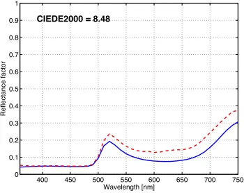
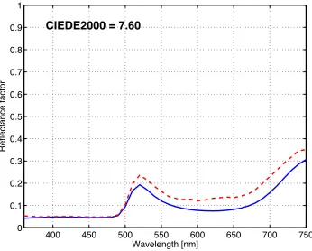
Figure 22. Spectral weights in the SCI for Hansa Yellow Opaque. 58

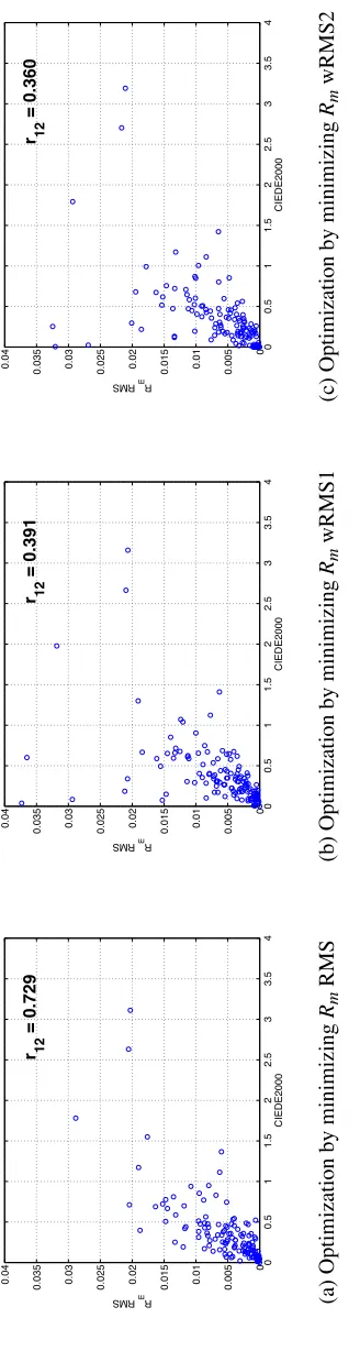
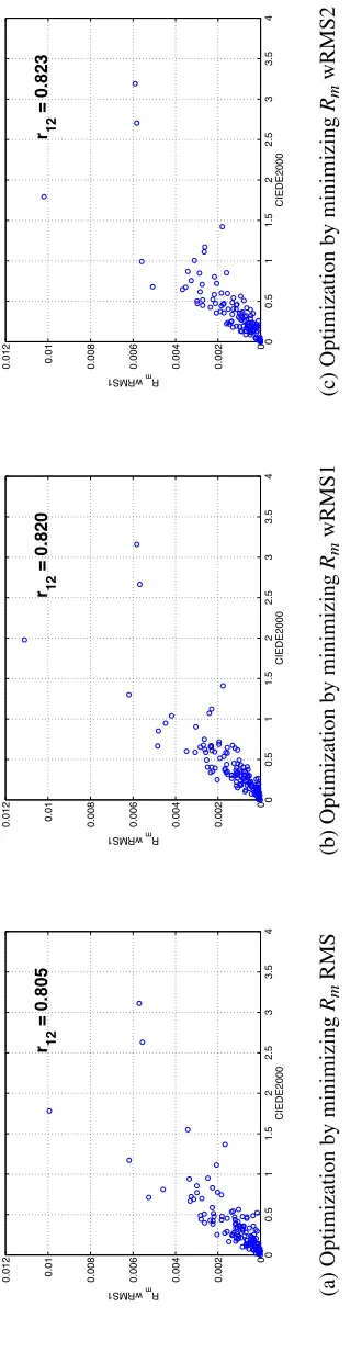
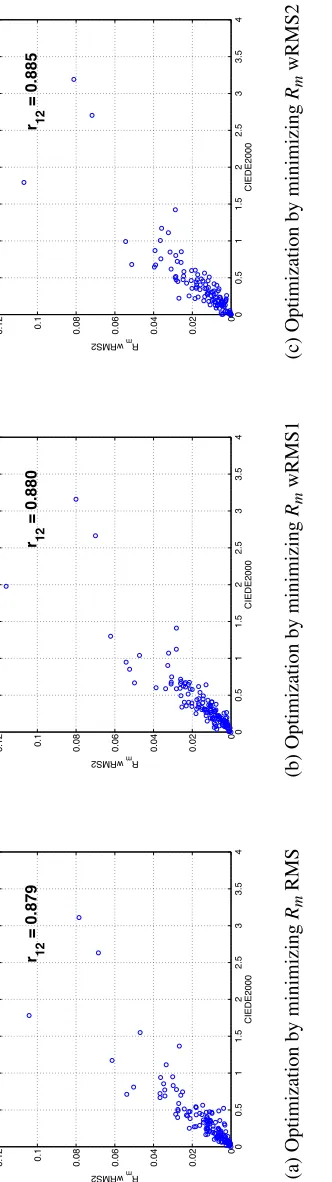
Figure 23. Correlation of characterization errors between CIEDE2000 and RMS. 65

Figure 24. Correlation of characterization errors between CIEDE2000 and wRMS1. 66

Figure 25. Correlation of characterization errors between CIEDE2000 and wRMS2. 67

Chapter 5: Paint Mixing Model Performance

Figure 26. The recipes of paint mixtures for verifying simulation performance. 69

Figure 27. Colorimetric plots for secondary mixtures between measurements and estimations. 70

Figure 28. Worst 6 of the spectral errors for secondary mixtures. 72

Figure 29. Reflectance change by a paint film thickness. 74

Figure 30. Simulation of opacity effects onto the spectral reflectance cueve of masstone

by reducing the unit k of Hansa Yellow Opaque. 75

Figure 31. Improvement of the secondary mixture estimation by an opacity change for the

previous worst five mixtures. 76

Chapter 6: Rendering Artist Paintʼs Color Gamut

Figure 32. Data filtering process from Step 2 to Step 3. 80

Figure 33. Rendering color gamuts for two three-primary paint sets. 81

Figure 34. The effects of an extra green paint addition for color gamut expansion for Case I. 83 Figure 35. The effects of an extra green paint addition for color gamut expansion for Case II. 84

Figure 36. Segmentation for global color gamut. 86

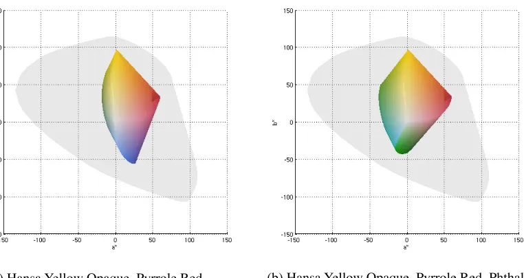
Figure 37. Chromatic plots for 27 acrylic paints. 87

Figure 38. Paint color gamut by using all the 26 colorants and a tint. 88

Figure 39. Extrapolation drawing by the Matlab function, “convhull”. 90

Chapter 7: Modeling Gloss Effects by Varnishing

Figure 41. Spectrophotomeric measurements for the tint ladders of Carbon Black

in the SPIN mode. 94

Figure 42. Spectrophotomeric measurements for the tint ladders of Carbon Black

in the SPEX mode. 96

Figure 43. Spectrophotomeric measurements for the non-varnished tint ladders of

Carbon Black. 97

Figure 44. Spectrophotomeric measurements for the varnished tint ladders of Carbon Black. 98 Figure 45. Correlation between the differences of specular gloss and the average spectral

reflectance differences for Carbon Black. 100

Figure 46. Worst estimation performance for the masstone of Phthalo Blue (Green Shade). 102 Figure 47. Color gamut expansion by varnishing based on the gloss simulation

v. LIST OF TABLES

Chapter 1: Introduction Chapter 2: Background

Table I. Deviation of the Saunderson correction. 15

Table II. Specular gloss levels and appropriate gloss geometries. 39

Chapter 3: Sample Preparation

Table III. List of GOLDEN paint names, C.I. names, and pigment names. 43

Table IV. GOLDEN acrylic paints and Gamblin oil paints haveing the identical pigments. 45

Chapter 4: Optimizing Paint Mixing Model Coefficients

Table V. The two-constant theory vs. the single-constant theory in characterization

performance. 54

Table VI. List of acrylic paints having maximum chroma and their colorant concentrations. 61

Table VII. Summary of the optimization approaches and their details. 62

Table VIII. Characterization performances for the paint database based on optimization

approaches. 63

Table IX. Correlation ratings between CIEDE2000 and spectral error matricies for global

optimization methods. 68

Chapter 5: Paint Mixing Model Performance

Table X. The statistical data of the estimation errors in CIEDE2000 for secondary

mixtures and individual paints. 71

Chapter 6: Rendering Artist Paintsʼ Color Gamut

Chapter 7: Modeling Gloss Effects By Varnishing

Table XII. The statistical data of CIEDE2000 color difference between non-varnished

paint specimens and varnished paint specimens in the SPIN mode. 95

Table XIII. Specular gloss measurement for Carbon Black. 99

Chapter 8: Summary and Conclusion Chapter 9: References

Chapter 10: Appendices

Table A-I. Recipes of paint drawdowns used for the artist paint database. 115

Table A-IIa. Colorimetric values in SPIN under D65 illuminant and the 1931 standard observer. 120 Table A-IIb. Colorimetric values in SPEX under D65 illuminant and the 1931 standard observer. 124 Table A-IIc. Colorimetric values in SPIN under illuminant A and the 1931 standard observer. 128 Table A-IId. Colorimetric values in SPEX under illuminant A and the 1931 standard observer. 132 Table A-III. Measurement values of specular gloss for the artist paint material database. 136

Table A-IV. Recipes of Secondary Mixtures. 140

Table C-I. Data formats of the measured reflectance factors for the database. 146

Table C-II. Data files of the measured reflectance factors for the database. 148

Table C-III. Data formats of the optimized paint mixing model coefficients for the database. 148

Table C-IV. The indexing number of each paint for the database. 149

Table C-V. Data files of the optimized unit ks and unit ss for the database. 149

Table E-I. Spectral characterization performances by local optimization. 160

Table E-II. Spectral characterization performances by global optimization (least square method). 161 Table E-III. Spectral characterization performances by global optimization

(least square - max chroma). 162

Table E-IV. Spectral characterization performances by global optimization (Rm RMS). 163 Table E-V. Spectral characterization performances by global optimization (Rm wRMS1). 164 Table E-VI. Spectral characterization performances by global optimization (Rm wRMS2). 165

Table G-I. Instruction on paint drawdown preparation. 172

CHAPTER 1. INTRODUCTION

As the project of the authorʼs Masterʼs thesis, the development of a spectral and colo-rimetric database of artist paint materials for arcylic paints was started. The goal of this research project was to:

- provide the academic resource of colorant spectral characteristics - give scientifc explanations on various paint-particular phenomena (paint mixing, gloss effects and color gamut expansion by varnishing)

These tasks were planned to satisfy possible interests on paint research from not only conservators in museums but also color educators in schools and color reproduction engineers in imaging companies.

First of all, the coverage of this research was narrowed down to matte acrylic paints that are made from traditional organic and synthetic pigments. That is, the paints of relatively brand-new colorants, fluorescent, metallic, and pearlescent pig-ments, were not considered herein.

aging researchers in a couple of ways. According to the recent study on the spectral-imaging camera system by Mohammadi and Berns [Mohammadi 2004], for example, it clarified that appropriate spectral-reflectance curves of a calibration target should be chosen rather than increasing the number of target paints for spectrally accurate calibration. For such a case, a colorant formulation using the spectral dataset will lead to determining the optimal recipes of acrylic paints providing appropriate reflectance curves to the development of a calibration paint target. Another possible usage of the spectral dataset is for pigment identification, the spectral matching technique of which is to find the recipes of paint mixtures, used in art, from a large amount of colorant spectral information.

The second mission was to simulate paint mixtures with mathematical calculations and verify the accuracy of the simulation performance. The simulation approach, based on the Kubelka-Munk theory, can be considered to have larger possible choices of paints and give better simulation results than gained by a traditional approach based on a look-up table method that characterizes a paint gradient in the L*a*b* coordinates [Carabott 2002]. The spectral-based technique of paint mixing simula-tion is expected to reveal the contradicsimula-tion of advocated paint-mixing theory, “yellow, red, and blue can make any colors because these colors are the primaries of the paint system”, to color educators because it is acually not. With regard to paint mixing theory, a professional artist, Michael Wilcox, experientially showed the contradiction by making a large amount of paint mixing palettes [Wilcox 2001].

compare color gamut volumes in the L*a*b* space among various coloration sys-tems including the paint system. A general target for calibrating cameras such as the GretagMacbeth ColorChecker is expected to cover a wide gamut far beyond a paint system. Quantifying the color gamut volumes of the systems would be helpful not only estimate color reproduction accuracy but also to develop a paint-color rendering chart for spectral imaging camera.

CHAPTER 2. BACKGROUND

2.1. Overview

This chapter summarizes the result of literature reviews on several optical principles of paint systems. To understand the whole range of the listed sections below is of assistance not only to build up such a colorant database but also to solve some enig-mas on the visual appearances of artist paintings that we are going to clarify in this research.

2.2 Color Mixing Theory for Artist Paints 2.3 Physical Theories on Gloss Effects 2.4 Physics and Color Science on Varnishing

2.5 Techniques of Paint Color and Glossiness Measurements

The first section is about color mixing theory in the paint system. This section introduces about how to characterize a large number of colorants mathematically with modern computational approaches. The keywords of this section are “Kubelka-Munk

theory”, “Saunderson correction”, and “non-linear optimization”.

The second section discusses about gloss modeling. Not only appearance but also measurement values by spectrophotomeric and colorimetric instruments are changed by the gloss effects. On “Fresnelʼs law of reflection” and “dichromatic reflection

model” are to be mentioned that helps paint researchers to recognize how spectral

curves of reflectance by gloss.

by varnishing.

2.2. Color Mixing Theory for Artist Paints

2.2.1. Kubelka-Munk Theory

The Kubelka-Munk theory is a mathematical model characterizing the internal reflec-tance of a paint medium. The model hypothesizes that light flux absorption and scat-tering occur in upward and downward directions perpendicular to the medium [Allen 1980; Haase 1992]. Figure 1 is the illustration explaining the optical phenomenon, where i and j are the identifiers of light flowing in two directions. While i represents a light flow moving towards the substrate, j indicates a light flow going up to the top. And then, in this figure, the upper direction from 0 to X is defined as positive in distance. At the specific depth, x, of a paint layer, when the incident light passes through the sub-layer of a small thickness dx, the amount of light penetrating down-wards decreases in proportion to absorption and scattering properties. The attenuation is expressed by Equation (2.1), consisting of two Kubelka-Munk coefficients, where

K is an absorption coefficient and S is a scattering coefficient. Both of the coefficients are assumed to be constant within the depth of a paint layer.

dx i

j

Paint Layer

x= X

x= 0 Light Source

Substrate

(

K

+

S

)

i dx

A light flux reaching the substrate (e.g. canvas) is bounced off and changes its direc-tion upwards. When the reflecdirec-tion light passes through at the sub-layer, the flux also decreases as the following:

(

K

+

S

)

j dx

By integrating these equations, the total amount of attenuation in each of the up-down directions can be calculated. For example, the light i is not only attenuated by the absorption and scattering of a colorant but also imposed by the light some part of the reflected light j because of scattering. Allen (1980) explained the formulation of such an optical interaction and solved the equations in his reference. By focusing on the two-flux directions, we obtain a pair of the differential equations:

di

=

(

K

+

S

)

i dx

�

Sj dx

�

dj

=

(

K

+

S

)

j dx

�

Si dx

These equations can be solved by replacing the ratio (i/j) with a single coefficient, ρ,

and those are to be united into a single equation:

d

�

dx

=

d

(

j

/

i

)

dx

=

i

(

dj

/

dx

)

�

j

(

di

/

dx

)

i

The ratios, (di/dx) and (dj/dx), are already given by transforming Equation (2.3). Now, therefore, we get a first-order equation consisting of K and S:

d

�

As the second step, we are required to think of ρ or the ratio (j/i), which are changed by corresponding with the depth x. Just remember, ρ represents the ratio of the returning light flux to the incident light. That is, ρ is equivalent to reflectance at a corresponding depth. When a depth x is equal to X (at the surface), it can be inter-preted that ρ is equal to the reflectance of a paint film, R. On the other hand, when x is equal to 0 (at the substrate), ρ must be equivalent to the reflectance of the substrate,

Rg, itself. With taking that into account, the equation for R can be solved and obtained as the following:

R

=

1

�

R

(

a

�

b

coth

bSX

)

a

�

R

+

b

coth

bSX

where

a

=

1

+

(

K

/

S

),

b

=

(

a

�

1)

This comprehensive equation is rarely used because paint researchers sometimes meet difficulty in measuring the thickness of an actual paint layer. Therefore, some simplified equation are introduced in response to specific conditions or manners. One situation is, if a specimen does not show any scattering property like a plastic film, Equation (2.6) is transformed into:

R

=

R

e

(

S

�

0)

The situation, in which Equation (2.8) is satisfied, is referred to as Bouguer-Beer law

Another situation is the case of analyzing a opaque sample represented as a ceram-ic title. According to the Kubelka-Munk theory, opaque intends the situation that the incident light cannot reach the substrate because of the strong opacity of a paint layer. That is, it is reasonable to consider that the thickness of a paint layer is infinite in this case. Thus, Equation (2.6) is simplified by giving X an infinite number and then can be changed into:

R

�

=

1

+

(

K

/

S

)

�

[(

K

/

S

)

+

2(

K

/

S

)]

(

X

� �

)

where R∞ is the reflectance of an opaque specimen (or the reflectance at an infinite

film thickness). This equation is also solved for K/S into a function of R∞:

K

/

S

=

(1

�

R

�

)

2

/ 2

R

� (2.10)

The concept which we have mentioned about so far is applicable to the case of determining a single K and a single S for an individual colorant. When allowing for the mixture of various colorants with different absorption and scattering properties ([k1, k2, ..., kn] and [s1, s2, ..., sn]; n is the number of colorants), we need to sum up all those properties somehow leading to being behaved as a unit colorant. Considering of such a paint mixing, it is necessary to correlate internal reflection with absorption coefficients and scattering coefficients.

One of the approaches is to assume the additivity of each of absorption and scatter-ing capabilities individually. The mathematical expression for the additivity appears in Equation (2.11):

K

=

(1

�

p

)

k

+

c

k

+

c

k

+

� � �

+

c

k

where t represents a tint, kt and st are the absorption and scattering coefficients of a tint respectively. And, ci is a theoretical concentration by weight for ith colorant, p is the sum of colorant concentrations, and n is the number of colorants mixed:

p

=

c

+

c

+

� � �

+

c

(0

�

p

�

1)

where p must be less than 1 because the sum of all the paint concentrations is 1. The formulation of supporting this hypothesis is called the two-constant Kubelka-Munk theory. In this colorant formulation, we are required to evaluate an absorp-tion coefficient and a scattering coefficient for each substance forming a paint layer. Therefore, K/S is driven by Equation (2.13):

K

S

=

(1

�

p

)

k

+

c

k

+

c

k

+

� � �

+

c

k

(1

�

p

)

s

+

c

s

+

c

s

+

� � �

+

c

s

In general, the two-constant Kubelka-Munk theory predicts the (K/S) of a paint pre-cisely.

Another approach is to assume the constancy of a absorption-scattering ratio (K/S) for each colorant. That is, a colorant is characterized by unit (k/s) instead of separate unit k and unit s. If we attempt to suppose that scattering coefficients, s1, s2, …, sn, are equal to st, Equation (2.13) can be simplified:

K

S

=

(1

�

p

)

k

+

c

k

+

c

k

+

� � �

+

c

k

s

equation of this approach is written:

K

S

=

(1

�

p

)

k

s

�

�

�

�

�

�

+

c

k

s

�

�

�

�

�

�

+

c

k

s

�

�

�

�

�

�

+

� � �

+

c

k

s

�

�

�

�

�

�

This equation implies the additivity of every (k/s). The formulation on this hypothesis is called the single-constant Kubelka-Munk theory.

In a pilot study, we figured out that the single-constant Kubelka-Munk theory did not show good estimation performance for our paint targets. The problem is that scat-tering properties at all the wavelengths were changed in response to the increase of a colorant percentage. Therefore, all the paints in this research were characterized by the two-constant Kubelka-Munk theory.

For the estimation of Kubelka-Munk coefficients, the tint ladder method was used. In this method, mixtures of a colorant with a tint are made at different concentrations. That is, tint ladders prepared are expected to show the wide range of a paint color from Titanium White to a masstone. Since the absorption and scattering of a tint, to which those of a colorant are characterized relatively, are denoted as the standard, a low-absorption high-scattering paint, Titanium White, is commonly used as a tint. The tint ladders are measured in reflectance factor and then converted to (K/S) by Equation (2.10) and the Saunderson Correction (cf. 2.2.2 Saunderson Correction).

Now, we are going to estimate k1 and s1 for a target paint by computation with the tint ladder method. For mixtures of two paints, a target paint and Titanium White, Equation (2.13) is simplified:

(

K

/

S

)

=

[

c

k

where the subscript i is the identifier of the i th tint ladder. Equation (2.16) consists of two unknown coefficients, k1 and s1. Equation (2.16) can be transformed into Equa-tion (2.17).

c

k

1

�

c

(

K

/

S

)

s

=

(1�

c

)[(

K

/

S

)

s

�

k

]

Furthermore, Equation (2.17) can be rewritten using a matrix equation as the follow-ing.

d

=

Cx

: general expression

(1

�

c

)[(

K

/

S

)

S

�

k

]

=

[

c

�

c

(

K

/

S

)

]

k

1

s

1

�

�

�

�

�

�

If we have two tint ladders except for a tint, Equation (2.18) can be solved si-multaneously. If we have more than three different concentration series including a tint, moreover, using least square method is to give optimal k1 and s1 values. In this case, the k1 and s1 of an independent matrix in Equation (2.18), x , shall be non-nega-tive. To satisfy this inequality constraint, we used a Matlab optimizing function,

“lsqnonneg“, in the computation. The algorithm details of Nonnegative Least Squares

(NNLS) are introduced in the reference [Lawson 1995].

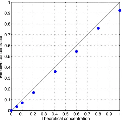
fit a relationship between theoretical concentration and effective concentration, least squares is also used. The plots of Figure 2 show the relationship for Carbon Black of GOLDEN matte fluid acrylic paints in the two-constant Kubelka-Munk theory. It can be observed that effective concentrations are underestimated comparing to theoretical concentrations in this case.

0 0.1 0.2 0.3 0.4 0.5 0.6 0.7 0.8 0.9 1 0

0.1 0.2 0.3 0.4 0.5 0.6 0.7 0.8 0.9 1

Theoretical concentration

Ef

fe

ct

iv

e

co

nc

en

tra

tio

n

Figure 2. A relationship between theoretical concentration and effective concentration.

After testing the importance of using the effective concentration, it was determined that most of the paints showed linearity for the theoretical concentration under the two-constant Kubelka-Munk theory. Thus, it was determined that the effective con-centration was not necessary for this research.

2.2.2. Saunderson Correction

spectrophotometer includes the effects of specular reflection so that it is hard to exclude only internal reflection from the measurement mechanically. We need to extract only internal reflection, R∞, expressed in Equation (2.9), therefore, when using

the Kubelka-Munk theory for paint characterization. In order to separate a measured reflectance into the two components, characterizing surface reflection is necessary. Surface reflection is characterized by the Saunderson equation. As mentioned in the previous section of “Fresnelʼs law of reflection”, first-surface reflection is character-ized by the ratio of two different refractive indices like air (1.00) and water (1.33). If a canvas is coated with a paint of 1.50 refractive index, 4% of an incident light will be reflected from the paint surface over all the wavelengths. Now, we can define this reflectance as K1. The rest of the light penetrates the surface and then bounces many times between the surface and the substrate. The amount of the penetrating light is defined as (1-K1). If the light bounced from the top does not scatter at all, the ratio of reflectance on the boundary between an air and a paint layer would be equal to K1 constantly. However, in the process of a light traveling in the medium, it is scattered in the advancing so that the reflectance at the top boundary characterized as a diffuse reflection ratio, K2, shows commonly a higher value than K1. The light flow so far is illustrated in Figure 3, that is the first-cycle stage including (1), (2), and (3). This mul-tiple reflection is continued into the second-cycle stage of (4), (5) and (6), the third, and so on.

Paint Layer

Canvas

(1) (4)

(3) (6) (2) (5)

(7)

(9)

R∞

Table II summarizes the derivation of the Saunderson correction [Allen 1980]. The blue terms in the second column represent the components of specular and diffuse reflections, the sum of which are detected by a spectrophotometer.

Table I. Deviation of the Saunderson correction.

Cycle _{from the surface}Light leaving Light penetrating_{into the substrate from the substrate}Light bouncing

1 (1) K1 (2) 1 - K1 (3) (1 - K1) R∞

2 (4) (1 - K1)(1 - K2) R∞ (5) (1 - K1) K2 R∞ (6) (1 - K1) K2 R∞2

3 (7) (1 - K1)(1 - K2) R∞2 (8) (1 - K1) K22 R∞2 (9) (1 - K1) K22 R∞3

... ... ... ...

It depends on measurement geometry, however, whether or not a specular compo-nent (1) is included in measurement values. By summing up all the compocompo-nents in the second column that is equivalent to reflectance by the specular component included (SPIN) measurement with an integrating sphere instrument, we can describe the mea-sured reflectance, Rm, as:

R

=

K

1

+

(

1

�

K

)

(

1

�

K

)

R

1

+

K

R

+

K

R

� 2

+

� � �

(

)

=

K

1

+

1

�

K

(

)

1

�

K

(

)

R

�

1

�

K

2

R

(2.19)

On the other hand, if we do spectrophotomeric measurements in the specular com-ponent excluded (SPEX) mode, first-surface reflectance is to be excluded. Hence, the final reflectance will come to:

R

=

1

�

K

1

(

)

1

�

K

2

(

)

R

�

where Rm indicates a measured reflectance.

As a matter of fact, even though the SPEX mode is selected, it is hard to eliminate only the effects of specular reflection completely because a specular trap may ex-clude only some portion of a diffused specular reflection trapped with a specular port

[Wyble 2003]. If specular exclusion in spectral measurements is necessary as much as possible, using the 45/0 geometry and employing Equation (2.20) will be the best way for the Kubelka-Munk solution.

The explanation so far is only valid for the simple paint coat that consists of three layers, air, a paint layer, and a substrate. However, the more complex structure of a paint coat should be discussed when characterizing the optical properties of variety of artist paint materials. One of the good examples is the varnish coat.

Berns derived the general mathematical equation of an optical model for the varnish coat from the Fresnel law of reflection [Berns 2003]. The model (c.f. “2.4.2

Surface Roughness”) allows a larger number of the optical properties than the

Saunderson equation does:

- The illumination angle of incidence

- Refractive indices of the varnish resin and paint-layer surface - Spectral transmittance of the varnish

- Internal spectral reflectance of the paint layer

2.2.3. Optimization Techniques For The Kubelka-Munk Solution

As mentioned in the previous chapter, least-square method is a powerful technique to estimate the Kubelka-Munk coefficients. The only problem of using this method is, however, obtained unit k and unit s for a colorant might not be desired values satisfy-ing an ideal spectral-error criterion. As shown in Equation (2.18), the non-negative least-square solution minimizes the residual, ||d - Cx||, at each wavelength. That is, estimated unit k and unit s for a target paint are expected to minimize root-mean-square (RMS) errors in K/S, not RMS errors in reflectance, Rm. The goal of the coef-ficients optimization is to make reflectance errors as small as possible so that colo-rimetric errors are to be minimized simultaneously. The relationship between a Rm error and a K/S error must show some correlation. From Equation (2.9) and Equation (2.17), Rm can be expressed as a function of K/S:

R

=

f

(

K

/

S

)

By manipulating this mathematical expression, the differential of Rm can be obtained as the following equation:

d R

=

�

R

�

(

K

/

S

)

d

(

K

/

S

)

Rm. In terms of optimizing an criterion, the blue line in the figure says that, minimiz-ing K/S errors weights Rm errors at high Rm, not at low-middle Rm.

0 0.1 0.2 0.3 0.4 0.5 0.6 0.7 0.8 0.9 1

- 1200 - 1000 - 800 - 600 - 400 - 200 0

Rm

∂

R

m

/

∂

(K

/S

)

Figure 4. A relationship between the sensitivity of measured reflectance and changes in K/S.

�����������

������

������������

������ �����

���������

����������������

�����������������

������

������������� ��

���

���

�����

������

����������� ��������������

��������������������������

�������������������

������������� ������ ������������ �������������������

����������������������� ���������������������������

This optimization workflow implies that the estimated Rm, j (jth tint ladder) is a function of Kubelka-Munk coefficients, Saunderson coefficients, and a theoretical concentration as shown in Equation (2.23):

ˆ

R

=

f

(unit

k

, unit

s

,

K

,

K

,

c

)

where unit k and unit s are the absorption and scattering coefficients of the two-con-stant Kubelka-Munk theory, K1 and K2 are the Saunderson coefficients, ci is a theo-retical concentration.

Kubelka-Munk coefficients, unit kj and unit sj (at jth wavelength), and Saunderson coefficients, K1 and K2, are simultaneously optimized. For the non-linear optimiza-tion, our approach is that, the initial values, unit ki and unit si, are pre-assigned the solution from the non-negative least-square method in Equation (2.18). At the same time, while the initial value of K2 is assigned an empirical value, 0.6, the initial value of K1 is assigned the minimum reflectance of the tint ladders over all the wavelengths. From experience, the masstone of a colorant have the minimum reflectance in the spectral region because of strong absorption. And then, those initial values are con-verted into K/S values first, and then into Rm values for each of tint ladders. After this computation, a RMS value between measurement and estimation for ith tint ladder is calculated by using Equation (2.24):

RMS

=

1

N

{ ˆ

R

(

�

)

�

R

(

�

)}

j=1 N

where N is the number of wavelengths in spectral measurement. After that, the aver-age RMS for a colorant is calculated:

RMS

=

1

M

(RMS

)

i=1

M

�

where M is the number of the tint ladders used.

If the average RMS is under a tolerance, the optimization process ends. If not, the initial values are tuned, and then the process continues from the starting point.

2.3. Physical Theories on Gloss Effects

In general, gloss is an optical phenomenon in which a surface luster or brightness is observed on a glossy object. Gloss finish (e.g. furniture and floor) gives people the sense of luxury, smoothness, and permanence. An impression from gloss directly affects observersʼ judgments to select the preferable appearance of colors rather than colors themselves in automotive and home appliance products. A color repro-duction system is no exception at this point. A good example of gloss preference is a photo-quality paper designed for inkjet prints that is categorized by three gloss levels: glossy, semi-gloss, and matte. Each gloss level gives you the different final appearance of a reproduced picture. A matte paper is used to emphasize the embossed texture of a paper ground so as to avoid undesirable sheen. On the other hand, a gloss paper produces high contrast, saturated images. Gloss is a familiar topic for photo consumers in daily life.

This section is to discuss about not only how gloss looks like (appearance) but also scientific explanations on gloss (theory).

2.3.1. Gloss Observation

When looking around our living environment, we might notice that there are a lot of objects artificially made glossy by changing their original appearances. One example is a framed poster with a plastic or glass plate on the surface. The flat structure of a glass plate bounces off the projection image of a lighting towards our eyes.

sys-tem was made of an inkjet print and a transparent plastic film. Covering a target photo printed on a semi-gloss paper with an OHP film made the appearance more glossy. A test photo was printed with a Canon S9000 inkjet printer. It is a general explanation on surface reflection that, once the incident light arrives at the film surface, some of the light beam is bounced off directly to the direction of mirror reflection without dif-fusion. At the same time, the rest of the light penetrates into the coloration medium.

Now, we are going to look at the appearance of a glossy target carefully under a diffuse lighting (Figure 6-(a)). The appearance viewed through a transparent film is more shining because of specular reflection at the film surface as shown in Figure 6-(c). And then, if you tilt it toward or off you without moving a viewing point, the amount of specular reflection will be dramatically changed in a range between gloss and haze. The contrast of perceived specular is getting larger when looking through the transparent film rather than through no film (Figure 6-(b)). It is also interesting that luminance density perceived is higher in dark tone through the film. When look-ing at the same figure, you might notice that the area where people gatherlook-ing in the back room is a darkest location in the scene. Corresponding with a darkening effect, colors come to being more saturated. We observed the dark spot through the transpar-ent film that a shade is compressed and tends to be much darker. The reason of dark-ening is associated with how much specular reflection an observer sees. However, colors in highlight are not significantly changed.

surface area because of the homogeneous intrusion of specular reflection. As a result, it can be observed a lower contrast image than the original.

A difference of gloss finish in our demonstration samples comes from the differ-ence in refractive index (RI) between air and a plastic film, or air and print paper. The different optical property prevents a few percentages of the incident light from penetrating the boundary. As a consequence, some portion of the incident light flux is reflected back to our eyes without any color absorption in an ink-dye layer. The details of physical theory on surface reflection, “Fresnelʼs law of reflection”, is to be explained in the next section.

(a) Lighting environment (b) Without a plastic film

(c) Glossy photo (d) Matte photo

2.3.2. Fresnelʼs Law of Reflection

Fresnelʼs law of reflection is an optical model of first-surface reflection, which is bounced off at the boundary between two media of different refractive indices. In this theory, normal incident light is simply attenuated by the ratio of reflection to incidence or reflectance expressed in Equation (2.18), where n1 and n2 represent the

refractive indices of two materials like air and a glass.

In addition to for normal incidence, the theory characterizes the total reflectance for multi-angle incidents, ρT, as a function of incidence angle, i, and the refractive

indices of the media, n1 and n2. Now, we hypothesize a collimated incident light. The

amount of first-surface reflection is expressed by the integration of two reflection components: reflectance for a polarized light oriented to the horizon, ρ||, and

reflec-tance for a polarized light oriented to the surface, ρ⊥. These reflectances are given

in Equation (2.19) and (2.20) respectively. The reflectance ρ||increases

monotoni-cally corresponding a increase of incident anglei. On the contrary, the reflectance

ρ⊥ decreases gradually to zero in the range from 0˚ to the critical angle. And then,

it increases exponentially with an increase of incident angle in the rest of the range. Equation (2.21) is given in order to calculate the critical angle f by using n1 and n2.

The critical angle is that, a polarized beam to the surface at a incident angle f is not reflected at all but penetrates completely. By taking the average of these reflectances, reflectance ρT for unpolarized incident light is finally gained in Equation (2.22). The

state of the whole features so far is shown in Figure 7. All the plots are obtained by assuming that (n2/n1) is 1.5.

Now, letʼs move on to looking at the case of a change in relative refractive index (n2/n1). Figure 8 shows relationship between reflectance ρT, relative refractive index,

higher reflectance. The interesting feature of the figure is also that, whatever relative refractive index is, ρT is constant within a range from 0˚ to 40˚ in incident angle.

�

=

n

�

n

n

2

+

n

�

�

�

�

�

�

�||

=

cos

i

�

(

n

/

n

)

�

sin

i

cos

i

+

(

n

2

/

n

)

�

sin

i

�

�

�

�

�

�

�

�

�

=

(

n

2

/

n

)

cos

i

�

(

n

2

/

n

)

�

sin

i

(

n

2

/

n

)

cos

i

+

(

n

2

/

n

)

�

sin

i

�

�

�

�

�

�

�

�

sin

f

=

n

n

(2.21)

�

=

(

�

+

�

) / 2

0 10 20 30 40 50 60 70 80 90

0 0.1 0.2 0.3 0.4 0.5 0.6 0.7 0.8 0.9 1

Angle of incident, i

Reflectance,

�

�_||

�_T

�_�

0 10 20 30 40 50 60 70 80 90 0

0.1 0.2 0.3 0.4 0.5 0.6 0.7 0.8 0.9 1

Angle of incident, i

R

ef

le

ct

an

ce

,

ρT

1.9 1.7

1.1 1.5

1.3

Figure 8. Fresnel reflection for unpolarized light based on incident angle,

i, reflectance, ρT, refractive index, n (from higher to lower reflectance,

n = 1.9, 1.7, 1.5, 1.3, 1.1).

As discussed so far, the amount of first-surface reflection under a directional il-lumination can be explained by Fresnelʼs law of reflection. That is, the theory can be considered to apply for 45/0 geometry measurements. However, the question is that, what would happen if supposing a diffuse illumination, which is the typical illumina-tion setting for integrating-sphere instruments, instead of a direcillumina-tional illuminaillumina-tion. We are interested in the effects of surface reflection onto spectrophotomeric mea-surements. To characterize the optical effects of vanish based on spectrophotometry, understanding the illumination-geometry influence onto spectrophotomeric measure-ments is necessary. Therefore, Fresnelʼs law of reflection must be extended to apply for a diffuse illumination.

expressed as the following Equation:

�

(

µ

)

=

1

2

a

�

µ

a

+ µ

�

�

�

�

�

�

+

n

µ

�

a

n

µ +

a

�

�

�

�

�

�

�

�

�

�

�

�

�

�

µ =

cos

i

,

a

=

n

�

sin

i

,

n

=

n

2

/

n

To compute the total reflectance in Equation (2.23) for a diffuse illumination, the equation is driven into Equation (2.25). Since dµ is changed from 0 to 1 that corre-sponds to a change in angle from 0 to π/2, the integration factor is multiplied by 2 to cover the entire incident angle from 0 to π.

�

=

2

�

(µ)

µ

dµ

1

�

theoreti-cally predictable from Figure 9 how many percentages of specular reflection are to be included in integrating-sphere measurement.

1 1.2 1.4 1.6 1.8 2

0 0.05 0.1 0.15 0.2 0.25 0.3 0.35 0.4

n

Fresnel reflectance

Normal incidence Diffused illumination

Figure 9. Fresnel reflectances for normal incident light and diffuse illumination.

2.3.3. Dichromatic Reflection Model

enter-ing a paint layer bounces off many times among pigment particles and binder resins and then returns to the surface. If the material shows perfect random scattering, the surface is called as Lambertian surface. A polytetrafluoroethylene (PTFE) tablet used for spetrophotometer calibration is one example of the Lambertian-like reflectors. The color of body reflection is determined by the absorption of pigments. The mathemati-cal equation of the model is expressed:

(2.21)

L(�,i,e,g)=L_surface(�,i,e,g)+L_body(�,i,e,g)

L is the light flux reflected from the material whereas Lsurface and Lbody are the light fluxes of first-surface reflection and body reflection respectively. Figure 10 explains each of geometry angles (i, e, g) of the equation where a bold arrow indicates normal direction to the surface. λ is the wavelength of a lighting spectra.

i e

g

surface normal

Figure 10. Scheme of explaining a viewing geometry where i is an incident angle, e is a detection angle, g is the phase between incident and detection directions.

to this assumption, each of unique reflection factors is decomposed into a factor of wavelength and that of geometry.

(2.22)

L(�,i,e,g)=m_i(i,e,g)c_i(�)+m_b(i,e,g)c_b(�)

In this simplified equation, mi (i,e,g) and mb (i,e,g) are the geometric scalars of first-surface reflection and body reflection (0 ≤ _{mi, mb} ≤ _{1), ci(λ) and cb(λ) are the}

spectrum of surface reflection and body reflection, respectively.

The dichromatic reflection model can be transformed to a simplified model when supposing spectrophotomeric measurements with a integrating sphere instrument. Since the geometry is diffuse geometry in our experiment, all the geometries are fixed somewhat in Equation (2.22), and the terms of geometry functions, mi (i,e,g) and mb

(i,e,g), are constants and then the equation can be transformed into:

(2.23) L_(�)=m

ici(�)+mbcb(�)

where L(λ) is the spectral power distribution (SPD) of the reflected light, and miand

2.3.4. Glossiness

The state of gloss is treated differently based on the appearance called “glossiness.”

The concept of glossiness is related to the specifications of spectrophotomeric mea-surement. A goniophotometer gives a full amount of reflectivity based on measure-ment geometries. The problem of using such a gonio instrumeasure-ment is the enormous amount of spectral reflectances at an innumerable combination of incident and detec-tion angles. In terms of quality control, therefore, a gloss index of lower dimension has been developed for paint manufacturing. Judd and Wyszecki in their book [Judd 1975] introduce five categories of different glossiness; (1) specular, (2) sheen, (3) contrast, (4) distinctness of image, and (5) absence of bloom. To categorize each gloss state, incident angle, viewing angle, and the beam size of illumination have to be de-termined. All of them are quantified by the ratio of luminance between standard and a trial specimen at a specific geometry. Among various gloss definitions available, the degree of specular or specular gloss is commonly used as a gloss index in the paint industry.

2.4. Physics and Color Science on Varnishing

2.4.1. Refractive Indices of Artist Materials

A couple of optical phenomena that are associated with different refractive indices of artist materials can be considered.

In general, after solvent evaporation, the structure of a dried paint is condensed tightly enough to stabilize pigments and binder resins, both of which have identical or different RIs. As far as several types of varnishes are concerned, it will be noticed that varnish RIs vary because of different chemical compositions. We recognize from these facts that the appearance of a paint or a varnished paint is composed by compli-cated optical systems.

For example, the difference in refractive index between pigments and binder resins causes scattering in the medium. This case is applicable to the combination of Titani-um White pigments and an acrylic emulsion. Comparing to the RI of TitaniTitani-um Oxide (2.71), acrylic emulsion has obviously smaller RI (1.48) so that the large difference in RI increases scattering capability. Some portion of the incident light bounces around in the vehicle of pigments and binder resins back and forth in this manner (Figure.11). At the same time, the other portions are absorbed and captured within the fine crystals of pigments. The encapsulation of a light flux within a pigment crystal would be hap-pened when pigmentʼs RI is extremely higher than the binderʼs surrounding RI.

Additionally, the difference in refractive indices of air and a binder (or a varnish resin) causes surface reflection. An optimal varnish material used for picture varnish is expected to have the same RI as the binder. The basic requirement of varnish is to protect paintings from humidity, dust, and the other chemical pollutions by a thin film coat without changing the original appearance. Therefore, a pre-investigation on a binderʼs RI is required to be successful as a picture varnish.

Pigment

Binder

Figure 11. Light interactions in the medium.

0˚ 15˚ 30˚ 45˚ 60˚

refraction total internal reflection

nt: 1.00 (air)

ni: 1.48 (acrylic emulsion)

2.4.2. Surface Roughness

With the increase of the RI difference between air and a varnish layer (or a paint layer), the amount of a light reflected from the surface to a viewer increases. How-ever, the influence of surface roughness upon the appearance of a painting is more significant than that of RI differences. Not only the Fresnel reflection from the surface but also body reflection from a paint media that is diffused according to micro surface structures. We assume that, whether a surface is rough or smooth determines whether a specimen is gloss or matte respectively.

Berns and de la Rie analyzed the effects of RI and surface roughness on color appearance to prove the assumption [Berns 2003a]. According to their research, a var-nish RI affects high reflectance rather than low reflectance. The effects of varvar-nishing to diffuse reflectance factor had been formulated with the Ryde transmission equation that is introduce in their paper.

(2.24)

�total=�in air +�first surface

where

(2.25)

�in air =

(1��d,va)�in varnishT

(1��d,vpR)(1��d,vaR)��d,vp�d,vaT 2

smooth enough to yield mirror reflection because an isotropic surface makes surface reflection diffused to some extent. The result implied that, even though the large dif-ference in spectral curve was observed in high reflectance region, color difdif-ference caused by the spectral difference was less than 2 in L* under the worst case (1.47 RI varnish). The reason of the small difference in lightness was due to perceptive con-trast compression represented by a non-linear relationship of lightness perception to luminance. That is, the color appearance change of a paint sample by varnishing was almost indistinguishable.

On the contrary, to simulate two extremely different surface states, completely lev-eling roughness and completely replicating roughness, the researchers excluded the component of first surface reflection associating with the leveling from and added it associating with the replicating into the total reflection. That approach is equivalent to the simulation of different geometry measurements: SPEX for the leveling and SPIN for the replicating. A spectral curve of the complete replicating was equally higher at all wavelengths than that of complete leveling. Changes of colorimetric data based on the spectral curve differences appeared in L* and C*ab. With leveling of the surface,

lightness decreased as well as chroma increased. However, if replicating the surface, even if applying different RI varnishes, no significant difference appeared in colori-metric data.

2.4.3. Color Gamut Expansion by Varnishing

with sands on a glass plate so as to make the surface uneven. And then, the uneven surface was coated with different RI varnishes or nothing with different thicknesses. A positive photo film was inserted between the glasses as a coloration material. For this specimen, a light source illuminated the specimen from the backside, and a digi-tal camera, which was calibrated to work as a colorimeter, captured the light passed through on the other side.

The result of colorimetric analysis showed that the varnish maked the colors dark-en and lively in chroma (based on specular excluded measuremdark-ent). That is, a color gamut expanded by varnishing was observed according to this simulation. As the authors mentioned, however, there is the unreasoning phenomenon that an increase in lightness by varnishing should not have occured for bright colors. If a varnish coat on a paint film is actually exemplified instead of using such a transmission system, some percentage of a reflection flux from a paint layer shall be bounced off at the boundary because of different RIs. In other words, lightness for each of all the varnished paints is expected to be reduced. A ground glass without sand blast shows high scattering because of significant difference in RI between air and a varnish coat. It is reason-able to suppose that, on the other hand, difference in RI between sand particles and a varnish coating them is too slight to induce scattering. As a result, the amount of an incident light passing comes to being larger through a varnished ground glass than through a non-varnished ground glass.

2.5. Techniques of Paint Color and Glossiness Measurements

2.5.1. Spectrophotometer

Spectrophotomeric measurement is the fundamental process to quantify the reflec-tivity of a paint medium. Of the variety of geometry reflectometers available, an integrating sphere spectrophotometer (diff/8˚) with a specular port was used for this research. The main reason of this choice was our aim to collect all portions of diffuse surface reflection from a replicated or leveled surface structure formed by varnishing. In SPIN measurements, all the surface reflection is detected regardless of the different degree of light diffusion caused by surface roughness. On the other hand, SPEX ge-ometry eliminates not all but most surface reflection with a specular trap in measure-ment. Considering of dichromatic reflection model, difference in spectral reflectance between SPIN and SPEX is expected to be a constant value at all wavelengths. For a glossy surface, at most 5% of incident light, which is calculated by Fresnelʼs law of reflection, are added in SPIN measurements [Hunter 1987]. In other words, the offset amount can be considered to represent the surface roughness of a paint specimen.

the matte samples were almost identical regardless of whether SPIN or SPEX, those curves of glossy samples varied.

What is important is, no matter what specular mode is used, an integrating sphere cannot separate a spectrophotomeric curve into two components, first-surface reflec-tion and body reflecreflec-tion, when analyzing a rough surface material. Some operators might confuse the terminologies, first-surface reflection and body reflection with specular reflection and diffuse reflection, the later of which is actually separated in spectrophotomeric measurements.

2.5.2. Glossmeter

To quantify the gloss level of a paint surface, a glossmeter, which is commonly used for quality control, is required to be prepared. The basic structure of a glossmeter is standardized in ASTM 523. According to the standard, glossmeter geometries are 20˚, 60˚, and 85˚, each of which is selected by an instrument operator corresponding to the gloss level of a test specimen: paint, coating, and panel. Table II is the summary of gloss levels and their applicable geometries.

Table II. Specular gloss levels and appropriate gloss geometries.

Gloss level Appropriate geometry

Ordinary 60˚

60˚ gloss > 70 20˚

60˚ gloss < 10 85˚

a standard surface under the same geometric conditions” [ASTM D523, 1999].

Figure 13 shows the structure of a parallel-beam glossmeter. From the left, an incandescent light source, the beam of which is focused by condenser lens attached in front of the source, is used to illuminate the surface of a test specimen. A source field aperture controls the amount of the light passing through. A source lens next to the aperture collimates the beam onto the surface with an appropriate beam diameter for projection. At the surface boundary, the light reflected from the surface travels into the direction of mirror reflection. A receptor lens focuses the reflected beam into a receptor field aperture so as to build up a source mirror image. And then, the image is focused by a collector lens through a spectral correction filter onto a photo detector at the end.

Condenser Lens Source Field Aperture

Source Source Lens

Specimen

Receptor Lens

Collector Lens

Spectral Correction Filter Receptor Field

Aperture

Photodetector

Figure 13. Structure of a parallel-beam glossmeter.

C. Therefore, it can be easily assumed that there is high correlation between specular gloss in a glossmeter and luminance factor in a colorimeter.

According to the ASTM standard, primary standards used for glossmeter calibra-tion shall be made of highly polished, plane, black glass with a refractive index of 1.567 for the sodium D line (589 nm). The color of a standard tile, black, is expected to avoid an unexpected light absorption of colorants possibly happened as a result of body reflection. The reflection amount from the standard is normalized into 100, which is the standard value relative to the specular gloss of any test specimen. How-ever, a commercial glossmeter produced by BYK Gardner is calibrated with a work-ing standard (tile), which is produced for practical purposes to satisfy mass-produc-tion and low cost materials. For example, a BYK Gardner tri-micro-gloss meter in our laboratory must be calibrated with a black glass tile that indicate 92, 95, and 99 specular glosses at 20˚, 60˚, and 85˚ geometries respectively.

Before actual gloss measurement, the preparing size of a specimen need to be care-fully determined. If the size is too small, a beam spot projecting on the surface might go beyond it at a large specular angle. Equation (2.26) indicates the relationship be-tween spot long axis and measurement geometry, shown in the cosine equation:

r₌ d

cos_� (2.26)

d

0˚

1.06 d

20˚

2.00 d

60˚

11.47 d

85˚

Figure 14. Comparison of the beam spot projection.

CHAPTER 3. SAMPLE PREPARATION

This chapter introduces the basic information on artist paint materials and drawdown preparation in this research: GOLDEN Matte Fluid Acrylic Paints, GOLDEN MSA Gloss Varnish, and paint drawdowns.

3.1. GOLDEN Matte Fluid Acrylic Paints

The target materials for the artist paint database are matte acrylic paints. A typical acrylic paint consists of pigments, acrylic emulsion (binder), water (solvent), and several coating additives. The entire set of the GOLDEN acrylic paints, which were chosen for this research, has 26 color variations and a white. While some of the paints were made of single pigments, the other paints contain two or three pigments. Table III shows paint names and their containing pigments with Colour Index Name (C.I. Name).

Table III. List of GOLDEN paint names, C.I. names, and pigment names.

Paint Name C.I. Name Pigment Name

Hansa Yellow Opaque PY 74 Arylide Yellow 5GX

Diarylide Yellow PY 83 Diarylide Yellow HR-70

Pyrrole Red PR 254 Dipyrrolopyrrol

Naphthol Red Medium PR 5 Naphtol ITR

Quinacridone Crimson PR 206 / PR 202 Quinacridone

Quinacridone Magenta PR 122 Quinacridone

Dioxazine Purple PV 23 Carbazole Dioxazine

Ultramarine Blue PB 29 Polysulfide of Sodium-Alumino-Silicate

Cobalt Blue PB 26 Oxides of Cobalt and

Aluminum Cerulean Blue,

Chromium PB 36:1 Oxides of Cobalt andChromium

Phthalo Blue (Green Shade) PB 15:4 Copper Phthalocyanine

Phthalo Green (Blue Shade) PG 17 Chlorinated Copper

Phthalocyanine

Jenkins Green PBk 9 / PY 150 / PG 36 Amorphous Carbon

Nickel Complex Azo Brominated & Chlorina-Copper Phthalocyanine

Permanent Green Light PY 3 / PG 7 Arylide Yellow

Chlorinated Copper Phthalocyanine

Chromium Oxide Green PG 17 Anhydrous Chromium

Sesquioxide

Green Gold PY 150 / PG 36 / PY 3 Nickel Complex Azo

Brominated & Chlorinated-Copper Phthalocyanine

Yellow Ochre PY 43 Natural Hydrated Iron

Oxide

Raw Sienna PY 43 Natural Iron Oxide

Burnt Sienna PBr 7 Calcined Natural Iron Oxide

Red Oxide PR 101 Synthetic Red Iron Oxide

Burnt Umber PBr 7 Calcined Natural Iron Oxide

containing Manganese

Raw Umber PBr 7 Natural Iron Oxide

contain-ing Manganese

Paynes Gray PB 29 / PBk 7 Ultramarine Blue

Carbon Black

Carbon Black PBk 7 Nearly Pure

Amorphous-Carbon

Titan Buff PW 6 Titanium Dioxide Rutile

Zinc White PW 4 Zinc Oxide

We expect that some of the acrylic paints contain the same pigments as the line-up of Gamblin Conservation Colors. The reason is that the Gamblin paint line-line-up is a popular oil-paint set used for painting conservation in museums. The research on acrylic paints is expected to contribute to a future related-paint research on the pig-ment identifications of cultural heritage oil paintings (e.g. Van Goghʼs, Henri Matisse) with a spectral imaging system. Table I