Placement, visibility and coverage analysis of dynamic pan/tilt/zoom camera sensor networks

Rochester Institute of Technology

RIT Scholar Works

Theses

Thesis/Dissertation Collections

7-2006

Placement, visibility and coverage analysis of

dynamic pan/tilt/zoom camera sensor networks

John A. Ruppert

Follow this and additional works at:

http://scholarworks.rit.edu/theses

This Thesis is brought to you for free and open access by the Thesis/Dissertation Collections at RIT Scholar Works. It has been accepted for inclusion

in Theses by an authorized administrator of RIT Scholar Works. For more information, please contact

[email protected]

.

Recommended Citation

Placement, Visibility and Coverage Analysis of

Dynamic Pan/Tilt/Zoom Camera Sensor Networks

by

John

A.

Ruppert

A Thesis Submitted in Partial Fulfillment of the Requirements for the Degree of

Master of Science in Computer Engineering

Approved By:

Supervised by

Assistant Professor Dr

.

Shanchieh Jay Yang

Department of Computer Engineering

Kate Gleason College of Engineering

Rochester Institute of Technology

Rochester, New York

July

2006

Shanchieh Jay Yang

Dr. Shanchieh Jay Yang

Assistant Professor

Primary Adviser

Andreas Savakis

Dr. Andreas Savakis

Professor and Department Head, Department of Computer Engineering

Chris M. Homan

Dr. Chris Homan

Thesis Release Permission Form

Rochester Institute of Technology

Kate Gleason College of Engineering

Title: Placement, Visibility and Coverage Analysis of Dynamic Pan/Tilt/Zoom

Camera Sensor Networks

I, John A. Ruppert, hereby grant permission to the Wallace Memorial Library reporduce

my thesis in whole or part.

John Ruppert

John A. Ruppert

Dedication

Acknowledgments

I

would

like

to

thank

Dr. Shanchieh

Jay

Yang

for his

continued support and encouragement

throughout the

course of

this

work.

I

would also

like

to thank

Dr.

Andreas Savakis for

inspiring

my interest in

camera

networking

research and

Dr.

Chris Homan for

lending

his

Abstract

Multi-camera

vision systems

have important

application

in

a number of

fields,

including

robotics and security.

One

interesting

problem related

to

multi-camera vision systems

is

to

determine

the

effect of camera placement on

the

quality

of service provided

by

anetwork

of

Pan/Tilt/Zoom

(PTZ)

cameras with respect

to

a specific

image processing

application.

The

goal of

this

work

is

to

investigate

how

to

place a

team

of

PTZ

cameras,

potentially

used

for

collaborative

tasks,

such as

surveillance,

and analyze

the

dynamic

coverage

that

can

be

provided

by

them.

Computational

Geometry

approaches

to

various

formulations

of sensor placement prob

lems have been

shown

to

offer

very

elegant

solutions;

however,

they

often

involve

unre alistic assumptions about real-world

sensors,

such as

infinite sensing

range and

infinite

rotational speed.

Other

solutions

to

camera placement

have

attempted

to

account

for

the

constraints of real-world computer vision

applications,

but

offersolutions

that

are approx

imations

over a

discrete

problem space.

A

contributionof

this

work

is

an algorithm

for

camera placement

that

leverages Com

Contents

Dedication

in

Acknowledgments

iv

Abstract

Introduction

1.1

Related Work

'.

1.1.1

Sensor Networks

1

2

3

1.2

Coverage: Examples from

other

fields

3

1.3

Coverage

in

Sensor Networks

4

1.4

Sensors

with

Directional

Sensing

12

1.5

Time-varying

(Dynamic)

Coverage in Sensor Networks

13

1.6

Camera

Coverage Models

14

1.7

Sensor

Placement

16

1.8

Visibility

17

1.9

Covering

Problems

17

1.10

Camera

Placement

18

1.2

Thesis

Overview

19

2

Dynamic PTZ Camera Coverage Model

21

2.1

Pan/Tilt/Zoom Cameras

21

2.2

Camera Parameters

22

2.2.1

Format Size

22

2.2.2

Effective Pixel Size

23

2.2.3

Focal Length

24

2.2.4

Angle

of

View

25

2.2.5

Field

of

View

(FOV)

25

2.2.7

Spatial Resolution

27

2.3

Application Parameters

27

2.3.1

Object Size

27

2.3.2

Required Pixels

27

2.4

Camera Coverage Parameters

27

2.4.1

Minimum Spatial Resolution

28

2.4.2

Minimum

Application

Distance

28

2.4.3

Maximum

Application

Distance

29

2.5

Static PTZ Camera Coverage Model

29

2.6

Dynamic

PTZ

Camera Coverage Model

31

Camera

Placement

and

Visibility

Algorithms

34

3.1

Procedure

34

3.2

Camera Placement

Algorithm

35

3.3

Camera

Visibility

Algorithm

38

3.3.1

Ray Shooting

40

3.3.2

Polygon Intersection

41

3.3.3

Event Points

42

Simulated Environment

and

Analysis

of

Dynamic PTZ Camera Coverage

.

45

4.1

Simulated

Environment

45

4.1.1

Application

Specifications

45

4.1.2

Camera Specifications

46

4.1.3

Floor

plan

47

4. 1

.4

Coverage

Metrics

48

4. 1

.5

Area Coverage Analysis

49

4.1.6

Implementation

Details

54

4.2

Critical Variables

for Camera Placement

55

4.2.1

Partitioning

55

4.2.2

Adjustable Camera Parameters

58

4.2.3

Restrictions

on

Camera Placement

60

4.3

Strategies for Camera Placement

and

Parameter Adjustments

61

4.3.1

Efficiency

62

4.3.2

Practicality

63

4.3.3

Robustness

65

4.4.1

Angle Bisector

vs.

Midpoint

Partitioning

67

4.4.2

MIN

vs.

MID

vs.

MAX Angle

Partitioning

68

4.4.3

Camera Parameter

Tuning

70

4.4.4

Restrictions

on

Camera Placement

70

4.5

Limitations

71

5

Concluding

Remarks

77

5.1

Future Work

79

List

of

Figures

1.1

Observer

placement

for

the

Art

Gallery

Problem

4

1.2

Coverage Behaviors.

E,

G,

and

B

represent system

Elements,"Good

guy"

to

be

protected,

and

"Bad

guys"

to

be

engaged,

respectively.

The

circles

around system elementsrepresent

the

effective sensor/effectorengagement

radius.

[12]

5

1.3

(a)

point

coverage,

(b)

area

coverage,

(c)

barrier

coverage

[7]

6

1.4

Examples

of

0-1

sensor model:

(a)

uniform

disks

and

(b)

non-uniform

disks.

[15]

6

1.5

r-strip[3]

9

1.6

Sensor Field With Voronoi

Diagram

and

Maximal Breach

Path

(MBP).

[18]

10

1.7

Sensor Field With

Delaunay

Triangulation

and

Maximal Support

Path

(MSP).

[18]

11

1.8

Plane

target

sonar sensor model.

A

plane

is

represented

by

the

perpendic

ular

distance

r and orientation a.

The

shaded rectangle

indicates

a single

sonar sensor

located

at

the

position

(xs,ys,

6S

).

[20]

12

1.9

Camera Coverage Model

15

1.10 2D

Covering

(a)

Sample

P

and

Q,

(b)

Translated

Q

Covers

P

18

1.11

Illustration

of

the

reachable region

from

a camera

(black

disk)

location

on

the

polygon perimeter.

[10]

19

1.12 Left:The

polygon.

Middle:CeIIular

representationof

the

polygon.

Right:The

cell coverage of a camera

O

with

FoV

limits OA

and

OF

and visible

poly

gon

OABCDEF. The

dark

cells are

the

visibleones

from

camera

0.[ 10]

. .

20

2.1

Format

Size

[16]

22

2.2

Typical image

sensor sizes

(units

in

mm).

[16]

23

2.3

CCD

sensor

[29]

24

2.4

Focal length

[30]

24

2.6

Field

of

View

and

Depth

of

Field,

a and

j3

are

respectively

azimuth and

latitude

of

the

Field

of

View,

c

is

the

camera,

eg is

the

optical

axis,

and

the

frustum

defined

by

the

planesabb'a'

andedd'e'

is

the

Depth

of

Field

.

[10]

26

2.7

Minimum

Application Distance (w.r.t. Face

Detection/Recognition)

....

28

2.8

(a)

Static

cameracoverage model and

(b)

image

sensor parameters

30

2.9

Dynamic Camera Coverage Model:

(1)

Static

camera coverage with cam

eraoriented

toward

point

A,

(2)

Camera

rotates uT

degrees

to

point

in

the

direction

of

B

and

(3)

Sweeping

field

of view of

the

camera

(shaded region)

3 1

2.10 Circular Sector

32

2.11

Sweeping

FOV

33

3.1

Procedure

35

3.2

Camera Placement Algorithm

36

3.3

Polygon Triangulation

[31]

37

3.4

Camera Coverage

39

3.5

Camera

Visibility

Example

41

3.6

Camera

Visibility

Algorithm:

Intersection

42

3.7

Camera

Visibility

Algorithm: Event Points

43

3.8

Camera

Visibility

Algorithm:

Visibility

Polygon

44

4.1

(1)

Face breadth

and

(2)

Face height

[32]

46

4.2

Sony

EVI-D100 Camera Specifications

[28]

47

4.3

Sony

EVI-D100

Pan/Tilt

Range

[28]

48

4.4

(a)

A

typical

floor

plan and

(b)

its

polygonapproximations.

[10]

48

4.5

Angle

of

View

(H)

vs.

Focal Length

(Sony

EVI-D

100)

50

4.6

Coverage Area

vs.

Focal Length

(Sony

EVI-D 100

w.r.t.

Face

Detection)

. .

51

4.7

Circular

sectorarea analysis

(R=l)

52

4.8

Dynamic

camera coverage model areaanalysis

54

4.9

Types

of

Triangles:

(1)

acute,

(2)

obtuse,

(3)

right and

(4)

equiangular ...

56

4.10 Triangle Partitioning:

(1)

Angle

Bisector

vs.

(2)

Midpoint

57

4.11

Triangle Partitioning:

(1)

MIN

vs.

(2)

MID

vs.

(3)

MAX

57

4.12 Coverage Utilization

58

4.13

Adjustable

Zoom,

(1)

Maximum

zoom coverage and

(2)

Minimum

zoom

level

coverage

59

4.14 Dynamic Camera Coverage: Case

(I)

Minimum

Zoom,

Minimum Pan.

(1)

4.15 Dynamic Camera Coverage: Case

(II)

Minimum

Zoom,

Maximum

Pan.

(1)

Camera Placement

and

(2)

K-coverage

61

4.16 Dynamic Camera Coverage: Case

(III)

Maximum

Zoom,

Minimum Pan.

(1)

Camera Placement

and

(2)

K-coverage

62

4.17 Dynamic Camera Coverage: Case

(IV)

Maximum

Zoom,

Maximum

Pan.

(1)

Camera Placement

and

(2)

K-coverage

63

4.18

Practicality

64

4.19 Real-world Floor Plan Shapes

72

4.20 Effect

of

Triangle

Partitioning

Scheme

on

Efficiency

73

4.21

Effect

of

Triangle

Partitioning

Scheme

on

Practicality

73

4.22 Effect

of

Triangle

Partitioning

Scheme

on

Robustness

74

4.23 Effect

of

Camera Parameter

Tuning

on

Efficiency

74

4.24

Effect

of

Camera Parameter

Tuning

on

Practicality

75

4.25

Effect

of

Camera Parameter

Tuning

on

Robustness

75

4.26 Camera

Placement,

no restrictions

76

List

of

Tables

2.1

Typical image

circle sizes

[16]

23

4. 1

Face Detection Specifications

47

4.2

Horizontal

Angle

of

View

(Sony

EVI-D

100)

50

4.3

Focal Length

and

Corresponding

Coverage

Area

(Sony

EVI-D 100

w.r.t

Face

Detection)

52

4.4

Circular Sector Area Analysis

(R=l)

53

4.5

Dynamic

camera coverage model areaanalysis

55

4.6

Real-world Floor Plan Shapes

and

Sizes

66

4.7

Results

from Real-world Floor Plan Shapes

and

Sizes:

Partitioning

66

4.8

Real-world Floor Plan Shapes

and

Sizes

67

Chapter

1

Introduction

Recently,

there

has been increased

emphasis on video surveillance research

for

various pur

poses, e.g., to

avoid

theft

in

commerce and national security.

Video

surveillance systems

typically

consist ofmultiple videocameraswhich are used

to

monitor an environment.

Tra

ditional

video surveillance systems

have

been

controlled

by

human

operators or

have

used

regular camera rotation schemes

to

observeobjects

moving

within

the

field

of view of

the

cameras.

As networking

and

image processing

research

progresses,

more advanced sys

tems

are

being

developed

to

automate

the

process of video surveillance.

This

involves

the

development

of

networking

policies and

image processing

and computer vision algorithms

to

detect,

locate

and

track

an objectas

it

moves

through

an environment.

An important

concept of multi-camera systems

is measuring

the

quality

of service

it

provides.

This

could

include,

for

example,

how

wella network of camerasensors monitors

an areaor

how effectively it

can

detect intruders.

The

focus

of

this

work

is

to

investigate

the

coverage provided

by

a network of

Pan/Tilt/Zoom

cameras.

A PTZ

camera

is

one

that

has

motorized control

for rotating

the

camera

in

all

di

rections as well as

zooming in

on an

image. This

work attempts

to

pair

up

aset of

PTZ

cameras withan

image processing

application

to

see

the

effects on coverage of

the

camera

set when

taking

into

account

the

constraints of a specific application.

The

question

this

work addresses

is:

How

may

one place a network of

PTZ

cameras,

The

key

challenge

here is

that

PTZ

cameras

may

adjust

their pan, tilt

and zoom

levels

over

time

andcooperate

in

order

to

improve

networkcoverage.

This

work

does

not attempt

to

provide anoptimal solution

to the

problem posed

above,

but

rather

the

goal

is

to

develop

a reasonable approach

to

gain

insight into

the

problem and

learn from

experience.

The

results of

this

work

include:

1.

A study

of

the

related work

2.

Static

and

dynamic

models

for

camera coverage

3.

An

algorithm

for

automated camera placement

that

places cameras

in

a room

that

provides complete coverage of

the

area of

interest

4. An

algorithm

for

camera

visibility

to

deal

with occlusion of walls withinaroomand

to

compute

the

overlapping

coverage

5.

A

simulatedenvironment and coverage metrics

for

implementing

and

testing

camera

coveragealgorithms

6. Camera

placement and parameter adjustment strategies used

to target

a particular

coveragegoal

1.1

Related

Work

At first

glance of

the problem,

it is

unclear

how

to

model

dynamic

coverage

for

a

PTZ

camera,

not

to

mention

gaining insight

on

how

to

placecameras

that

have dynamic

coverage capabilities.

So,

a

starting

point

for

this

research was

to

determine

what

it

means

to

model

"coverage".

This

section summarizes

the

related work

study,

highlights important

concepts

1.1.1

Sensor

Networks

The

emergence of sensor networks as a premier research

topic

is

a

key

motivating factor

for

this

work.

Sensor

networks

have been

made possible

by

recent advances

in

communi

cations and embedded

micro-sensing

technologies.

A

sensor network consists ofanumber

of sensors nodes

that

collaborate

to

perform a

larger sensing

task

and

to

communicate

the

information

to

a

sink,

or a central

location [2]. Sensor

nodes are small electronic

devices

equipped with one or more

sensors,

a

transceiver,

storage

components,

processing

com

ponents and

possibly

an actuator.

The

low-cost, low-power,

multi-function capabilities

of sensor nodes enables unique

features,

such as random

deployment

and collaborative

sensing.

These features

allow

for

a wide range of potential applications and

thus

makesen

sornetworks an

interesting

topic

for

research.

Exemplary

applications

include battlefield

surveillance,

forest fire

detection,

smart environments and

inventory

control.

This

work

considers a network of

PTZ

camerasensors

targeting

image processing

applications.

1.1.2

Coverage: Examples from

other

fields

Coverage

is

an

important

concept

that

will

be drawn

upon

in

this

work.

The

term

"cover

age"

typically

refers

to

measures ofeffectivenesswhich are used

to

characterize

the

overall

performance of a system.

The

idea

of

"coverage"

appears

in

a number ofapplications

in

various research

fields,

including

the

Art

Gallery

Problem

[24],

satellite ocean

monitoring

[13]

and

the

coordinated

positioning

of mobile robots

[12].

The Art

Gallery

Problem

involves

determining

the

number and

locations

ofobservers

needed

to

monitor

the

interior

of an n-wall art

gallery

room such

that

every

point

in

the

room

is

seen

by

at

least

one observer.

Using

computational

geometry,

it has been

shown

that

[f

J

observers

is occasionally necessary

and always sufficient

to

guard an art

gallery

with n vertices

in its

polygonal representation.

Quite

often notall of

the

|_

J

observers are

needed.

For

example,

consider

the two

polygons

in Figure 1.1

each with

12

vertices,

one

n=

13

[n/3J=4

n=12 Ln/3j= 4

Figure 1.1: Observer

placement

for

the

Art

Gallery

Problem.

The

question

then

becomes: How

can one

determine

algorithms

for

minimumguard place

ment?

Research has

shown

this type

of problem

to

be NP-hard [24].

In

[13],

satellites are used

for

coverage of global oceans

to

determine

the

abundance

ofphytoplankton.

The

authors of

this

work

define

"coverage"

as percentage of

the

ocean

surface

that

can

be

monitored

in

a single

day.

A

method

is

presented

to

improve

ocean

coverage

by

exploiting redundancy in information from

various missions.

This

is done

by

collecting

and

merging information from

satellitesat various orbits.

The

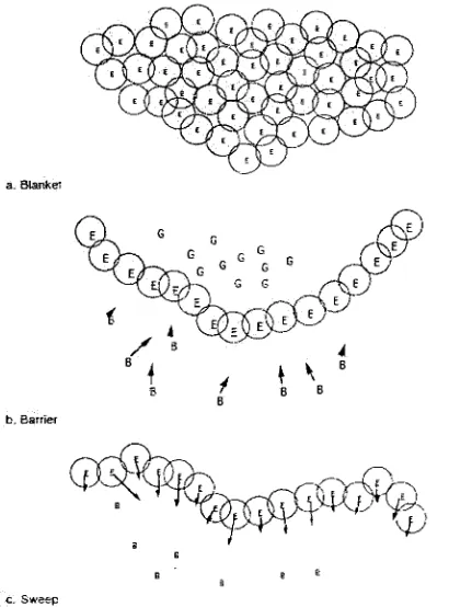
concept of

"coordinated positioning

and movement

in

concert"

for

command con

trol

of many-robot systems

is

considered

in

[12].

Here,

"coverage" refers

to

maintaining

a spatial

relationship

between

mobile robots with respect

to

a specific mission goal.

The

author

defines

three types

of coverage:

(1)

blanket

coverage,

(2)

barrier

coverage and

(3)

sweep

coverage.

Figure 1.2

illustrates

these

coverage

behaviors.

Blanket

coverage refers

to

determining

a staticarrangement of elements

that

maximizes

the total

amount of area covered.

Barrier

coverage also

involves

a static arrangement of

elements,

but

its

goal

is

to

minimize

the

probability

that

penetration

through the

barrier

willgo undetected.

Lastly,

the

objectiveof

sweep

coverage

is

to

move a

group

ofelements

across an area of

interest

taking

into

account

the trade

off

between maximizing

the

area

coveredand

minimizing

the

number of missed

detections

perunit area.

1.1.3

Coverage in Sensor Networks

Coverage

is

alsoan

important

concept

in

sensor networks

and,

since

the

applications

being

[image:18.540.170.375.74.351.2]

c._Sweep

Figure 1.2: Coverage Behaviors.

E, G,

and

B

represent system

Elements,

"Good

guy"

to

be

protected,

and

"Bad

guys"

to

be

engaged,

respectively.

The

circles around system elements represent

the

effective sensor/effector engagement radius.

[12]

great

detail how

coverage

has been defined for

sensor networks.

The

coverage problem

in

sensor networks

is

centered around

quantifying

the

quality

with which sensors monitor a physical space.

Due

to the

variety

of available sensors and

the

numerous applications of sensor

networks,

many different formulations

of

the

coverage

problem

have been

proposed

by

the

research community.

The

most studied

types

ofsensor

network coverage

include

the

following

subjects:

(1)

point

coverage,

(2)

area coverage and

(3)

barrier

coverage.

Figure 1.3 illustrates

each of

these

concepts.

The

following

section presents some

typical

models used

for sensing

and

discusses

in detail

the types

of coverage

illustrated in Figure 1.3.

In

addition,

some examples of

,--"""o

""'.

o

: O 6

x

^?c~o--pa

v>>

u

'

\

X

'

0 ..'-..

O' L'T"

.

?'"';.

o o.on o

o

(a) (h) (cl

Figure 1.3:

(a)

point

coverage,

(b)

area

coverage,

(c)

barrier

coverage

[7]

Sensor Models

Many

formulations

of

the

coverage problem use sensor models as a

starting

point

for

the

definition

ofnetwork coverage.

The

most

basic

sensor model proposed

in

the

literature

is

a

disk

model where

the

radius of

the

disk

represents

the

sensing

range of

the

sensor

[15].

This

type

of model will

be

referred

to

as

the

0-1

sensor model

throughout this

work.

Figure

1.4

illustrates

the

0-1

sensor model

for

sensors with

both

uniformand non-uniform

sensing

ranges.

Figure

1.4:

Examples

of

0-1

sensor model:

(a)

uniform

disks

and

(b)

non-uniform

disks.

[15]

More

complex senor models

that take

into

account

the

uncertainty

of sensors

due

to

that

sensing ability

diminishes

as

the

distance between

a sensor anda

target

increases,

thus

a sensor

is

more

likely

to

detect

an event

happening

at acloser

distance

as opposed

to

a

distance further

away.

This

will

be

referred

to

as

the

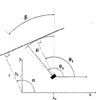
probabilistic sensor model.

Equation

1.1

is

anexampleof

how

such a sensor model

is formulated

mathematically.

S(s,p)

=

--^

(1.1)

Here,

d(s,

P)

is

the

Euclidean distance between

the

sensor 5 and

the

point

p,

and posi

tive

constants

A

and

K

are sensor

technology-dependent

parameters.

Deployment

In

addition

to the

sensormodel

used,

another

important

consideration

for

analysis of net

work coverage

is how

sensors are

deployed in

an environment.

Two

types

of

deployment

are

defined in

the

literature:

(1)

deterministic

and

(2)

random.

Deterministic

coverage

refers

to

coverage provided

by

a set of sensor nodes

deployed according

to

a predefined

layout.

The deployment

can

be

uniform or weighted

to

account

for

areas of

increased

network

activity,

or

hot

spots.

Examples

of uniform patterns

include

repeated geometric

patterns,

such as

square, triangle

and

hexagon. In

this case,

coverageanalysis simplifies

to

the

analysis of one

basic

cell

because

of

the

symmetric properties of

the

uniform pattern.

As

anexampleof weighted

deterministic

coverage,

considercameracoverageof valuable

items in

a museum.

To

ensure protection of more valuable

items,

an

increased

number of

cameras could

be

used

for monitoring

them.

It is

not always

feasible,

however,

to

place sensors

in

a

deterministic fashion. Consider

placing

nodes

in

a

battlefield

or a

disaster

area

for instance. In

such cases

it is

important

to

consider random

deployments. An

example of assumptions made

in

the

related work

is

Point-based

and

Area-based

Coverage

The

objective of point-based coverage

is

to

achieve a static arrangement of sensor nodes

such

that

eachpoint

in

a

discrete

set of points-of-interest

is

covered

by

at

least

onesensor

node at

any

point

in

time.

Figure 1.3

(a)

illustrates

the

goal of point coverage.

The

set

of points-of-interest

that

are required

to

be

covered are

depicted

as squares and

the

sensor

nodes are

depicted

as circles.

The

connected

black

nodes are active nodes and can ade

quately

cover

the target

points.

A scheduling

algorithm

for

consumption of

energy based

on

rotating

which nodes are active can

be

used

to

determine

which nodes should

be

active at

any

given

time

in

order

to

meet coverage requirements.

Area

coverage

is

an extension of point-based coverage and

focuses

on

monitoring

a particularareaorcontinuous set of points

in

the

physical world.

Figure 1.3

(b)

illustrates

the

area coverage concept.

The black

sensor nodes are used

to

represent

the

active sensor nodes and

the target

area

to

be

covered

is

the

large box. The

active nodes ensure

that

every

point within

the target

area

is

covered,

as opposed

to

Figure 1.3

(a)

in

which one

is only

concerned with

covering

a

few discrete

points.

The

analysis of point-based coverage

is

also applicable

to

area-based

coverage,

and vice versa.

The only

difference

is

the

subject

to

be

covered.

Next,

some example

formulations

for

point-based and area-based coverage of sensor networks with

both

deterministic

and random

deployments

are presented.

These

examples use

the

previously defined 0-1

sensor model

for

coverage analysis.

If

the

placement of sensor nodes can

be

achieved

exactly

as

planned, the

coverageprob

lem essentially

means

planning

the

placement of nodes

to

meet

desired

coverage require

ments.

In

this

case,

the

goal of coverage can

be,

for

example,

determining

the

minimum

number ofsensorsneeded

to

cover a given

discrete

setofpointssuch

that

every

target

point

is

covered

by

at

least

one

sensor,

as considered

by

the

authors

in [3].

formation

is

not

known,

the

algorithm

for maintaining

coverage

is

more complex.

This is

accomplished

by defining

disjoint

sets of sensor nodes such

that

every

set ofsensors nodes

provides complete coverage of

the target

points.

In

order

to

preserve

energy,

only

one of

the

sets

is

active at

any

given

time

and

the

sets are activates

in

a sequential order.

The

algorithm aims

to

determine

the

maximumnumber of

disjoint

sets so

that the time

between

activation ofaparticular sensor

is

thus

also maximized.

In

addition

to their

point

based

coverage

analysis,

the

authors

in

[3]

also consider plac

ing

a minimum number of sensor nodes

to

covera

target

area orcontinuous set ofpoints.

The

authors

define

the

conceptof an

r-strip,

or a

string

of

0-1

sensors

along

a

line

and use

it

to

analyze performance ratios

for bounded

convexregions.

This

concept

is illustrated in

Figure 1.5. For

more

details,

see

[3].

Figure 1.5:

r-strip

[3]

An

important

consideration

for

sensor network

design

is fault

tolerance.

Sensor

nodes

may fail due

to

lack

of

power,

physical

damage

or environmental

interference,

thus there

is

a need

for

redundancy

or

overlap

of

sensing

areas.

Many

different

applications require

varying degrees

of redundancy.

Coverage

analysis provides a

methodology in

which re

dundancy

can

be

quantified.

This

idea is

presented

in

terms

of acoverage

formulation for

randomareacoverage

in [15]. The

authors

define

the term

/c-coverage

to

refer

to the

cover

age

degree

where

k

represents

the

number of sensornodes

that

cover a particular area.

The

higher

the

value of

k,

the

more robust

the

network

is

to

sensor

failures

and

thus the

more

reliable

the

information

that

is

reported

to the

sink.

This

concept

is illustrated in Figure

Barrier Coverage

Barrier

coverage refers

to

determining

whether or not an event

may

pass across a

path,

or

barrier,

without

being

detected.

This

type

of coverage

in depicted in Figure 1.3

(c).

Various

types

of

barrier-based

coverage

have been

proposed.

Here,

two

such examples

arepresented.

In

[18],

the

authors combine an algorithmic approach with computational

geometry for

analysis ofcoverage

in

sensor networks.

The

key

ideas developed

are

the

concepts ofworst-case and

best-case

coverage.

The

objectives of worst-case coverage are

to

find

areasof

"lower

observability"

from

sensornodes and

to

detect

breach

regions.

Best-casecoverage

focuses

on

finding

areas of

"high

observability"

and

identifying

regions of

best

support.

The

authors

define

worst-case coverage as

the

maximal

breach

path

(MBP),

or

the

path

in

which

the

distance between any

point on

the

path and

the

closest senor node

is

maxi [image:23.540.172.372.375.504.2]

mized.

This

scenario

is illustrated in

Figure 1.6.

Figure 1.6: Sensor Field With Voronoi

Diagram

and

Maximal Breach Path (MBP).

[18]

This

concept exploits

the

idea

that

sensing

accuracy generally decreases

as

distance

from

asensor node

increases

(i.e.,

the

Probabilistic

sensor model).

The

maximal support path

(MSP),

or

best-case

coverage,

is

the

case where

the

distance

between

any

point on

the

path and

the

closest sensor node

is

minimized.

The MSP is

illustrated in Figure 1

.7.

The

concepts of

best

and worst-case coverage

highlight

weak

Figure

1.7:

Sensor Field With

Delaunay

Triangulation

and

Maximal

Support Path

(MSP).

[18]

and protocol

designers for future

node placement or node relocation.

Another

model

for barrier

coverage

is

the

exposure-based model.

This

concept was

introduced in

[19]

and

is built

upon

in [1]. This

model alsoassumes

that

sensing accuracy

diminishes

with

increased

distance,

but additionally

accounts

for

the

amount of

time

a

senor

is

exposed

to

an event.

Depending

on

the type

of

sensor,

an

integral

or

derivative

model

may be

used

to

determine

the

intensity

of

the

exposure.

This

intensity

value

is

then

used

to

develop

detection

models.

If

the

intensity

over a given

time

interval

exceedssome

threshold,

then the

event

is

detected,

otherwise

it is

not.

Analysis

of coverageproceeds

in

a

similar

fashion

to

[18]

in

that

it focuses

on

determining

best-case

and worst-case coverage

scenarios.

Best-case

coverage

is

the

path of maximal exposure and worst-case coverage

is

the

pathof minimal exposure.

Many

of

the

previously

mentioned

formulations do

wellat

thoroughly

defining

cover

age

for

either a specific

type

ofsensoror aspecific

application;

however,

there

has

not

been

much

focus

placed on

accounting for

variations

in

types

of sensorsand networkoperation.

Part

of

the

contribution of

this

work

is

to

provideageneral

framework for

coverage analysis

of a network of

Pan/Tilt/Zoom

cameras which

takes

into

account variations

in

the

factors

that

affect network coverage and condenses camera coverage

into

metrics

that

can

be

used

for

comparison ofnetworks ofcameras withvarious parameter settings and various modes

1.1.4

Sensors

with

Directional

Sensing

Most

of

the

previously

mentioned coverage

formulations

assume omni-directional

sensing

capabilities;

however,

there

are

many

types

of sensors

that

are

limited

to

directional

sensing.

For example,

consider sonar and camera sensorswhere

sensing is limited

to

anangle or

field

of view.

In

this

case

it is important

to

consider orientation of

the

sensors when

designing

algorithms and placement strategies.

Figure 1.8 illustrates

one example of a physics-based [image:25.540.192.348.228.390.2]

directional

model of a sonar sensor.

Figure 1.8: Plane

target

sonarsensor model.

A

plane

is

represented

by

the

perpendicular

distance

r and orientation a.

The

shaded rectangle

indicates

a single sonar sensor

located

at

the

position

(xs,

ys,0s)-

[20]

A

major contribution of

this

work will

be development

of a

directional sensing

model

for

the

analysisofcoveragewhen

using

cameras

for

sensing.

Typically,

related works

have

modeleda sensor's

sensing

rangeas a

disk,

where

the

radius of

the

disk is

the

sensing

range.

This

assumes

that there

is

no

direction

associated with sensor's

sensing

capabilities.

In

the

case of a

camera,

sensing

range

is

limited

by

the

field

of view and

therefore

has

a

direction

associated with

it. This

work attempts

to

incorporate directional sensing into

analysis of

1.1.5

Time-varying

(Dynamic)

Coverage in Sensor Networks

While

coverage of

immobile

sensors with omni-directional

sensing

capabilities

has been

extensively

explored and

is relatively

well

understood,

only recently have

researchers more

extensively

explored

the

idea

of

time-varying

or

dynamic

coverage

[5]. This

type

of net

work operation

may be desirable in

the

case of

having

a

limited

numberof sensor

nodes,

or when

it is

notrequired

to

cover

every

point of

the

area of

interest

simultaneously.

In

the

caseof

time-varying

coverage, the

sensing

area of a sensor node changes over

time.

As

a

result,

points

that

were

originally

uncovered

may

alternate

between

being

cov

ered and not

being

covered and

thus

a greater amount ofarea will

be

covered over

time.

This

bring

about

the

following

questions

to

be

answered

[5]:

What is

the

area coverage at a given

time

instant?

What

is

the

area coverage over a

time

interval?

What

are

the

durations

of

time that

a

location

is

covered and not covered?

Additionally,

for

static coverage of a sensor

network,

an

intruder

that

is

not

initially

detected

will never

be detected if it

remains

stationary

or moves

along

an uncovered path.

Detection

of

the

intruder is

more

likely

to

occur

if

sensorscan search an area.

This

concept

brings

about

the

following

important

questions

to

be

answered

by

this

work:

How quickly

can a network of

PTZ

cameras

detect

an

intruder?

How does

the

detection

time

depend

on

the

searching strategy

of

the

cameras?

Can

one

derive

camera-parameteradjustment strategies

to

improve intrusion detec

tion

capabilities?

In

[5],

the

authors show

that

mobility

can

be

used

to

offset a

lack

of sensors

in

order

to

improve

network coverage.

This

work will attempt

to

useadjustment of camera

instead

of

1.1.6

Camera Coverage

Models

An

additional contribution of

this

work will

be

the

development

of a model

for

coverage

ofa

PTZ

camera withrespect

to

image processing

application.

Camera

models are used

to

characterize

the

viewof a camera

using intrinsic

and extrinsic camera parameters

[17]. In

trinsic

camera parameters

specify internal

camera characteristics and

include focal

length,

principal point and effective pixel size.

Extrinsic

parameters

describe

the

spatial relation

ship between

the

camera and

the

world.

Exemplary

extrinsic parameters are

the

rotation

matrixand

translation

vector.

The

inputs

to

a camera model are

typically

defined

using

cameraparameters and

the

outputs represent

the

relationship between

a point

in

the

world reference

frame

and

its im

age projection.

One

suchexample

is

the

pinhole camera model

[17].

Here,

the

relationship

between

a

3D

point

M

and

its image

projection m

is

given

by

the

formula:

m =

A[Rt]M,

(1.2)

where

A is

the

camera

intrinsic

matrix,

R is

the

rotation matrix and

t

is

the translation

vector.

The

matrix

A

can

be

expressed as:

A

(

\

1

X

0

cx

^

0

Jy

cy

0

0

1

)

(1.3)

where

(cx,

cy)

are coordinates of

the

principal

point,

(fx,

fy)

are

the

focal lengths

by

the

axesx and

y

and

the

matrix

R

and vector

t

can

be

expressedas:

m

ri2

ru

R

'tl\

,

t

=

t2

\h

J

(1.4)

7~21

r22

T23

\

r3i

r32

r33

j

Other

camera models

have been developed

to

determine

the

degree

of

uncertainty

in

measurements obtained

from

acamera sensor.

In [1

1],

the

author

develops

acameramodel

to "gain

a

degree

of confirmation or

rejection"

based solely

on visual

information. This is

accomplished

by

extracting

room

features from

the

camera

image

and

comparing

them

with

features

extracted

from

apre-developed world

model.

Similar

to the

pinhole camera

model,

the

model

in

[11]

uses camera parameters as

inputs,

namely

a camera

image,

the

robot's

hypothesis

of

its

current position and

the

actual

position of

the

robot.

Unlike

the

pinhole camera

model,

however,

the

output of

this

model

is

the

probability

that the

robot's

hypothesis is

correct.

This

can

be

thought

ofas a

quality

ofservice measurement.

For

this work, the

goal of

the

camera model

is

to

characterize

the

coverage of a

PTZ

camera

in

the two-dimensional

world

using

the

focal length

and pan parameters of

the

camera as

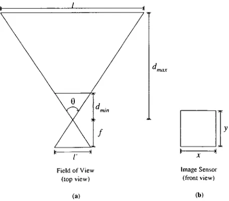
inputs. The

pan parameter will

define

the

orientation of

the

camera relative

to

some reference

frame,

similar

to the

0

or a parameter

illustrated in

the

sonar model

in

Figure 1.8. The

focal length

parameter sets

the

zoom

level

of

the camera, thus

a practical

limit

is imposed

on

the

view range

by

the

finite

spatial resolutionof

the

camera.

Figure 1.9

illustrates

apossible model

for

the

field

ofviewof a camera with a

limited

view range.

ImageSensor (frontview)

[image:28.540.157.385.382.582.2]

(a) (b)

Figure 1.9:

Camera Coverage Model

This

work

focuses

on coverage

in

two

different

aspects,

namely

area coverage and

How

can one model area coverage

for

a

PTZ

camera?

What is

the

criteria

for detection

ofan

intruder

(stationary

or mobile)?

How

can onemodel

detection

time

ofan

intruder?

A study

of

the

related workreveals

the

following

areas

in

which proposed camera mod

els

may be improved

upon:

Unrealistic Assumptions:

Computational

Geometry

models,

such as

those

pre

sented

in

[24],

make assumptions about

the

view of a camera

that

do

not

apply

to

real-world

cameras, e.g.,

infinite depth

of

field

and

infinite

rotational speed.

This

work

focuses

on

defining

the

real-world constraints

for modeling

camera coverage

for

a more practicaland realizable approach.

Off-line

vs.

On-line Placement

of

Cameras:

Many

active vision works

have

con

sidered cameraplacement

for

on-line

activity,

but

to

our

knowledge,

little

work

has

been done

on

the

off-lineplacement of cameras prior

to

performing

the

active vision

task.

Task-specific

constraints:

Camera quality

of servicerequirements

vary for different

tasks,

thus

there

is

a need

for

a generic camera model

that

incorporates

the

idea

of

task-specific parameters,

such as

the

minimumacceptable spatial resolution.

1.1.7

Sensor

Placement

For

multi-cameravision

systems,

as

the

size ofanetwork

increases,

it quickly becomes im

practical

for

network

designers

to

consider

placing

cameras

by

hand.

Thus,

it is important

to

consider algorithm

for

automated placement ofcameras.

Related

works,

such as

[10]

and

[23],

have

addressed

the

problem of

attempting

to

minimize

the

number of cameras

When

considering

real-world vision

applications,

it is important

to

consider

the

con

straints

that

limit

the

coverage

ability

ofa network of cameras.

For

example,

[10]

intro

duces

the

idea

of

constraining

camera placement

based

on

task-specific

and

floor

plan-specific coverage requirements.

In

[23],

the

authorsconsider

the

placementof static cam

eras

(sensors)

in

a

dynamic

scene.

A

contributionof

this

work

is

to

build

upon related work and consider

the

placementof

dynamic

cameras

in

astatic scenewhilealso

considering

constraints specific

to

aparticular

floor

plan or

image processing

application.

1.1.8

Visibility

Another

important

real-world consideration

that

needs

to

be

taken

into

account when con

sidering

the

coverage

ability

of multi-camera networks

is

constraints

imposed

by

the

pres

enceof obstacles within

the

region of

interest. This

could

include,

for

example,

poles or

walls within a

building

or an object

moving in front

of a camera and

occluding its field

of

view.

Analyzing

visibility becomes

increasingly

important

when

considering

sensors

that

can

vary

their

sensing

area over

time

and scenes

that

change over

time.

[23]

considers

the

effects on

visibility

of static cameras as a scene changes over

time.

This

work considers

the

visibility

of staticand

dynamic

camera coverage models with respect

to

static scenes.

1.1.9

Covering

Problems

Covering

problems aim

to

find

placements ofa network of sensors so

that, together,

they

coveracollection of

target

regions

[9].

For

example,

[8]

considers

2D covering

polygons

where

the

goal

is

to

decide

if

asetof

covering

polygons can

be

translated to

covera

target

set.

If

the

answer

is"yes",

then the

polygons are rotated and placed.

This is

illustrated

in

~

\VpJ>

/

o,

//

XX--V

\

(a)

[image:31.541.109.431.60.264.2]

(b)

Figure 1.10: 2D

Covering

(a)

Sample P

and

Q,

(b)

Translated

Q

Covers

P

This

workattempts

to

draw

upon

this

concept

by

using

cameras,

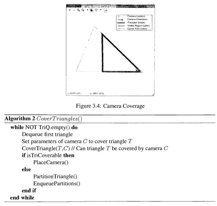
representedas

triangu

lar

regions, to

cover a polygon representation of a

floor

plan.

The

polygon

is decomposed

into

triangular

regions and

the

question

becomes,

given camera and application

constraints,

can one place acamera and adjust

its

parameterssuch

that the

camera covers

the triangle?

If

the

answer

is

"yes",

then the

camera

is

placedand

the

parameters are adjusted.

Another important

piece of

information learned

from

the

study

of

covering

problems

is

that

anumberof

2D covering

problems

have been

proved

to

be NP-complete [9]. This

gives an

idea

of

the

complexity

of

the

problem

being

dealt

with and

is

additional support

for

a

heuristic

approach.

1.1.10

Camera

Placement

Other

related works

have

studied

the

problem of camera placement and

have

proposed

solutions.

[10]

considersamore realistic model

for

acamera

than those

proposed

in Com

putational

Geometry

works such as

[24]. In

addition, the

authors

in

[10]

propose methods

for

incorporating

task-specific

constraints

into

amodel

for

camera coverage.

The

problem

is

posed as a

discrete

optimization problem where

the

goal

is

to

minimize

the

cost of plac

developed

in

[10]

that

will

be drawn

upon

in

this

thesis

include

the

formulation

of a model

for dynamic

camera coverageandconceptofvisibility.

The

authors presentamethod of

developing

amodel

for dynamic

camera coverage

that

involves

the

introduction

of a

task-specific

time

constraint.

This

represents

the

minimum

amount of

time

required

for

anobject

to

be

within

the

visible

field

of view of at

least

one

camera

in

the

system.

By determining

the

sweeping

angle of view of acamera over

time,

the

field

ofview of

the

cameracan

then

be

approximated

by

a

triangular

region.

Figure

1.11

illustrates

this

concept.

Figure 1.11: Illustration

of

the

reachable region

from

a camera

(black

disk)

location

on

the

polygon perimeter.

[10]

This

work attempts

to

simplify

this

dynamic

camera coverage model even

further

by

only considering

a partial range of motion

instead

of

considering sweeping

the

camera

over

the

entire range of motion.

Additionally,

the

authors

in

[10]

present a method

for

dealing

with occlusion of ob

jects,

or

determining

the

"visibility" of a camera.

To do this,

an angle

sweep

technique

is

presented.

While

this

work

heavily

leverages

this

concept,

the

implementation is vastly

different

in

that

[10]

works

in

the

discrete

space,

while

this

work attempts

to

work

in

the

continuous space.

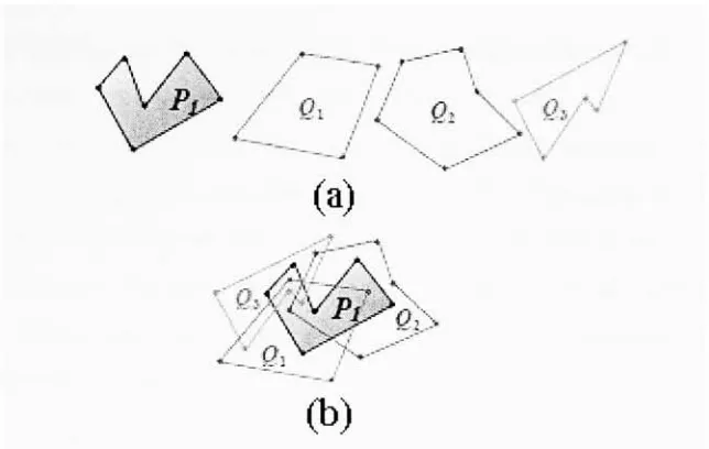
Figure 1.12 illustrates

the

concept ofpolygon

visibility

overa

discrete

problem space.

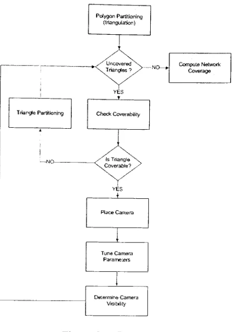
1.2

Thesis Overview

This

thesis

presentsan approach

to the

cameraplacementproblem

that

involves

determin

I

i

H

car:::::

j

It %

t

I

t f

o

Figure 1.12:

Left:The

polygon.

Middle:Cellular

representationof

the

polygon.

Right:The

cell coverage ofa camera

O

with

FoV limits OA

and

OF

and visible polygon

OABCDEF.

The dark

cells are

the

visibleones

from

camera

O.[10]

different

shapesof

triangles

(representing

the

field

of view of

the

cameras)

that

covera

2D

room and

analyzing

the

cameraplacement algorithm via simulations

to

gain

insights

as

to

Chapter

2

Dynamic

PTZ

Camera

Coverage Model

In

order

to

make

the

problem more

manageable, the

constraints of

the

problem can

be

relaxed

to

only

consider

two-dimensions.

Thus,

the tilt

aspectofa

PTZ

camera

is ignored.

Based

on

the

study

of

the

relatedworkand

this simplification,

it

seems

that

a

reasonable,

yet simple enough approach

is

to

model

the

dynamic

coverage of each

PTZ

camera as a

triangle

that

represents

the

field

of view of

the camera,

and place

different

shapes andsizes

of

triangles to

cover a

2-D

room.

The

approach

is

to

first

develop

a model

for

static camera

coverage,

and

then

extend

the

model

to

incorporate dynamic

coverage constraints.

The

goal

is

to

represent

the

sweeping

field

ofview of a camera

in

the

shape of a

triangle.

This

then

givesus

the

ability

to

analyze

a given camera placement

algorithm,

in

terms

of

the

efficiency, robustness,

and

practicality

of

the

coverage provided

by

the

network of

PTZ

cameras.

This

section outlines proposed model

for dynamic

camera coverage.

Here,

consider

the

2D

area

that

can

be

covered

by

a camera with respect

to

aparticular

image processing

application.

For

completeness,

some

important

terms

andcamera parametersareoutlined.

2.1

Pan/Tilt/Zoom

Cameras

Various

types

ofcameras are available

for

video surveillance

tasks.

This

work

focuses

on

Digital

camera:

A digital

camera uses an electronic sensor

to

acquire spatial vari

ations

in light

intensity

and

then

applies

image

processing

algorithms

to

the

data

provided

by

the

sensor

to

reconstructapictureof a scene

[4]. Two

technologies

cur

rently

used

to

manufacture

digital image

sensors are

Charge Coupled Device

(CCD)

and

Complementary

Metal Oxide Semiconductor

(CMOS). Both

CCD

and

CMOS

perform

the task

of

converting light energy into

electric charge

to

capture

informa

tion

about a scene.

Image

sensors can

be

thought

ofas a

2-D array

of

thousands

or

millions of

tiny

solarcells

that

each

transform

light

from

one small part of an

image

into

electrons.

Pan/Tilt/Zoom

(PTZ)

camera:

A

Pan/Tilt/Zoom

camera

is

a special

type

of camera

that

has

motorizedcontrol

for rotating

the

camera

in

all

directions

and

zooming in

on

an

image.

2.2

Camera Parameters

Next,

some

important

camera parameters are

defined.

2.2.1

Format

Size

An

ideal lens

produces

images in

the

form

of a

circle,

called

the

image

circle.

Digital

cameras use a rectangular

image

sensor

to

capture a scene

through

a

lens.

Figure 2.1

illustrates

the

concept of

format

size.

ImageCirclev

(mageSize

Vertical

Horizontal

The

ratio of

horizontal length

to

vertical

length

of

the

image

sensor

is known

as

the

aspect ratioof

the

camera.

A

typical

aspect ratio

is 4:3 (H:

V)

for

a standard

digital

camera.

Table 2. 1 displays

examples ofcommon

image

circle sizes

along

with

the

corresponding

horizontal

and vertical

lengths.

Image Circle

Horizontal

Vertical

04.0mm

3.2mm

2.4mm

06.0mm

4.8

mm

3.6mm

08.0mm

6.4mm

4.8mm

011.0mm

8.8mm

6.6mm

016.0mm

12.8mm

9.6mm

Table 2.1: Typical image

circle sizes

[16]

Lenses

are

designed

to

work with specific

image

sensor sizes.

Different

image

sensor

sizeswill yield

different

fields

of view

using

the

same

focal length. Common image

sensor

sizes

include

1/4", 1/3", 1/2",

2/3"and

1". Figure 2.2

illustrates

some

typical

image

sensor

sizes and

the

corresponding

horizontal,

vertical and

diagonal

lengths.

1/4"

HI2.4

3.2 1/3--43-'

1/r

?* .Sfit ,8

II

4.6 [image:36.540.189.356.389.524.2]

6.4 2/3" ,,s

m

6.6 X"6

m

9.6 8.8 12.8

Figure 2.2: Typical image

sensor sizes

(units

in

mm).

[16]

2.2.2

Effective Pixel Size

Most image

acquisition units

today

utilize

CCD

technology.

Compared

to

picture

tubes,

CCD devices have relatively lower

production costs and

have

the

advantage of

being

com

two-dimensional,

spatially discrete

image. Figure 2.3 illustrates

the

2-D array

nature ofa

CCD

sensor.

CCD. chip

Figure 2.3: CCD

sensor

[29]

An

important

parameterof

CCD

chips

is

resolution,

which

is

expressed as

the

number

of pixel elements.

A CCD chip

typically

has

a

few

rows and columnsof

"blind"

pixelsat

its

edges,

thus the

areaof

the

chip

used

for image

acquisition

is known

as

the

effective pixel

size of

the

chip.

An

example of a modern

high

resolution

CCD chip is

one

that

contains

756

pixels

in

the

horizontal direction

and

58 1

pixels

in

the

vertical

direction.

2.2.3

Focal Length

For

a

thin

double

convex

lens,

rays

from

an

infinite light

source will converge ata single

point,

called

the

focal

point.

The distance between

the

lens

and

the

focal

point

is known

as

the

focal length

f. To optimally

capture ascene atan

infinite distance

to

an

image

sensor,

the

distance between

the

lens

and

the

sensor

is

set

to the

focal

length,

i.e.,

the

sensor should

lie

on

the

focal

plane.

This

is illustrated in Figure 2.4 (a).

point oflight

(a)

<M

2.2.4

Angle

of

View

The

angle

of

view corresponds

to the

amount of a given scene

that

appears on a sensor.

Angle

ofviewcan

be

measured

horizontally,

vertically

or

diagonally.

For digital

cameras,

angle of view

is

a

function

of

focal length

and

the

size of

the

image

sensor

[16]. This

is

illustrated in Figure 2.5.

8}

;

/

\ /

>

/-CCDchip

/'

Figure 2.5: Angle

of

View

The formula for

angle of

view,

using

the

ideal lens

model,

is

represented

in Equation

2.5.

9

=

2

arctan(

yh

(2.1)

Here,

9

is

the

angleof

view,

/

is

the

focal

length

of

the camera,

and

V

is

a

dimension

of

the

CCD chip

(horizontal,

vertical or

diagonal).

See Figure 2.2 for

more

details..

With

a

fixed image

sensor

size, there

is

an

inverse,

non-linear

relationship between

the

focal length

and

the

angleof view.

2.2.5

Field

of

View

(FOV)

The

volumetric region visible

from

a camera

is defined

as

its field

of

view

[10].

This is

determined

by

the

apex angles of

the

pyramidalregion

originating from

the

lens

center of

x^\

l

\

;- -,/

\

!

"7bh

\

'j

/

Figure 2.6: Field

of

View

and

Depth

of

Field,

aand

/?

are

respectively

azimuthand

latitude

of

the

Field

of

View,

c

is

the camera,

eg is

the

optical

axis,

and

the

frustum defined

by

the

planes

abb'a'

andedd'e'

is

the

Depth

of

Field

.

[10]

2.2.6

Depth

of

Field

(DOF)

The

depth

of

field

ofa camera

is

the

distance between

the

nearest and

farthest

objects

that

appear

in acceptably sharp focus in

an

image [10]. This

concept

is illustrated in Figure 2.6

as

the

frustum defined

by

the

planes abde and a'b'd'e'.

Further

decomposing

DOF

into

two

components:

Minimum

Object Distance: The distance between

a camera and

the

nearest object

that

appears

in acceptably sharp focus is defined

as

the

minimum object

distance.

This is dependent

upon

the

camera's

focal length. The

greater

the

focal

length,

the

greater

the

minimumobject

distance.

Maximum Object Distance: The distance between

the

camera and

the

farthest

ob

ject

that

appears

in acceptably sharp focus defines

the

maximum object

distance.

This

parameter

is

dependent

upon task-specific

constraints,

which

may be

spatial,

temporal

or

based

on

quality

of service.

For

example,

consider

the

image

process

ing

applicationof

human face

detection.

In

this case, the

maximum object

distance

would

be limited

by

a minimumacceptablespatial resolutionof

face

images

required

2.2.7

Spatial

Resolution

Spatial Resolution is

a measure of

accuracy

or

detail

ofa

digital image. As

an

example,

for

a

digital

image,

this

could mean

the

ratio

between

the total

numberof pixels needed

to

representan object

in

an

image

and

the

size of

the

object

in

the

realworld.

The

higher

the

spatial

resolution,

the

more

detailed

and sharper an

image

will

be.

2.3

Application

Parameters

Because

this

workconsiders

the

coverageof acamerawith respect

to

an

image-processing

application,

here

some application-specific parameters are

defined.

2.3.1

Object Size

This defines

the

sizeof

the target

object

to

be

covered.

2.3.2

Required Pixels

This is

an application-specific constraint

that

defines

the

minimum pixelresolutionrequired

for

a particular

image-processing

algorithm.

2.4

Camera

Coverage Parameters

For

this work, the

problem

formulation

is limited

to two-dimensional

regions

in

order

to

make

the

problemmoremanageable.

The

camera coveragemodel

is defined in

terms

of

in

putsand outputs.

The

idea

is

to

convert

the

cameraparameters and

task-specific

constraints

of

the

problem

into

a spatial coverage representation.

In

order

to

do

this,

some additional

2.4.1

Minimum Spatial Resolution

The

minimum spatial resolution

parameter,

rs,

refers

to

an application-specific

limit

on

the

acceptable resolution of captured

images.

In

this

case,

consider applications such as

face detection

and

face

recognition.